A C2-continuous control-volume technique based on cartesian grids and two-node integrated-RBF elements for second-order elliptic problems

Cartesian grids and two-node integrated-RBF elements for

second-order elliptic problems

D.-A. An-Vo1, N. Mai-Duy1and T. Tran-Cong1

Abstract: This paper presents a new control-volume discretisation method, based on Cartesian grids and integrated-radial-basis-function elements (IRBFEs), for the solution of second-order elliptic problems in one and two dimensions. The gov-erning equation is discretised by means of the control-volume formulation and the division of the problem domain into non-overlapping control volumes is based on a Cartesian grid. Salient features of the present method include (i) an element is defined by two adjacent nodes on a grid line, (ii) the IRBF approximations on each element are constructed using only two RBF centres (a smallest RBF set) associated with the two nodes of the element and (iii) the IRBFE solution is C2 -continuous across the interface between two adjacent elements. The first feature guarantees consistency of the flux at control-volume faces. The second feature helps represent curved profiles between 2 adjacent nodes and leads to a sparse and banded system matrix, facilitating the employment of a large number of nodes. The third feature enhances the smoothness of element-based solutions, allowing a bet-ter estimation for the physical quantities involving derivatives. Numerical results indicate that (i) the proposed method can work with a wide range of the shape-parameter/RBF-width and (ii) the proposed technique yields more accurate results and faster convergence, especially for the approximation of derivatives, than the standard control-volume technique.

Keywords: integrated-radial-basis-function element, Cartesian grid, control-volume formulation, local approximation, second-order elliptic problem, C2-continuous so-lution.

1 Introduction

Traditional techniques used for solving second-order elliptic differential equations include overlapping finite difference methods (FDMs), non-overlapping finite el-ement methods (FEMs), boundary elel-ement methods (BEMs) and control volume methods (CVMs). These methods typically utilise polynomials as an interpolator. To avoid notorious polynomial snaking phenomena, low-order polynomials such as linear variations are widely used, usually leading to errors of order h2, where

h is the mesh spacing. For element-based solutions, only the approximating

func-tion (not its partial derivatives) is continuous across elements (i.e. C0continuity). The overall error can be reduced by using progressively denser meshes. A mesh needs be sufficiently fine to mitigate the effects of discontinuity of partial deriva-tives. It is thus desirable to have discretisation methods that can produce a solution of higher-order continuity across elements.

Radial basis functions (RBFs) have successfully been used for the approximation of scattered data over the last several decades. They have also emerged as an attrac-tive scheme for the numerical solution of ordinary and partial differential equations (ODEs and PDEs) (e.g. Fasshauer (2007) and references therein). Theoretically, some RBF-based methods can be as competitive as spectral methods; the two types of methods can exhibit spectral accuracy. Unlike pseudo-spectral techniques, they do not require the use of tensor products in constructing the approximations in two dimensions or more. The RBF approximations usually rely on a set of dis-tinct points rather than a set of small elements. When this characteristic is com-bined with the point-collocation formulation, the resultant discretisation methods are truly meshless (e.g. Kansa (1990)). RBF-based collocation methods can be applied to differential problems defined on irregular domains without added dif-ficulties. Apart from point-collocation, RBFs have also been employed as trial functions in other formulations such as the Galerkin, subregion collocation and in-verse statements, resulting in enhanced rates of convergence (O(hα)with α>2) of these approaches. Works in this research trend include Atluri, Han, and Rajen-dran (2004); Sellountos and Sequeira (2008); Orsini, Power, and Morvan (2008); Mohammadi (2008).

In a pivotal paper on function approximation by Franke (1982), it was pointed out that the multiquadric (MQ) RBF scheme yields the most accurate results. The present work employs the MQ whose form is defined by

gi(x) = q

(x₋ci)2_+a2

i, (1)

Tran-Cong (2003), the value of the shape parameter was simply chosen as ai=βhi withβ being a given positive number and hi the distance between ciand its nearest neighbour. When the direct way of computing the interpolants is used, RBF-based methods such as those using MQs are known to suffer from the so-called uncer-tainty principle. As the value ofβ increases, the error reduces while the matrix condition number increases undesirably. In practice, one desires to use largeβs up to a value at which the system matrix is still in good condition. RBF-based methods can be classified into two categories: global and local. Global methods use every RBF on the whole domain to construct the approximations at a point, resulting in a fully populated system matrix (c.f. Kansa (1990); Sarler (2005); Zerroukat, Power, and Chen (1998); Mai-Duy and Tran-Cong (2001)). When the number of RBF centres and/or the value ofβ increase, the condition of RBF matrices deteriorates rapidly. Such drawbacks typically render global methods unsuitable for complex problems, where many points are required for a proper simulation. In addition,

β to be used is confined to small values. For local methods (e.g. Tolstykh and Shirobokov (2003); Shu, Ding, and Yeo (2003); Lee, Liu, and Fan (2003); Šarler and Vertnik (2006); Divo and Kassab (2007); Sanyasiraju and Chandhini (2008); Mai-Duy and Tran-Cong (2009)), only a few RBFs are activated for the approx-imations at a point. The resultant system matrix is sparse and banded, which is suitable for handling large-scale problems. However, trade-offs include the loss of spectral accuracy and high-order continuity of the approximate solution. Var-ious schemes have been proposed to enhance the performance of local methods. Using large values ofβ appears to be an economical and effective way (Cheng, Golberg, Kansa, and Zammito (2003)). In the case of non-overlapping domain-decompositions, where a large problem is replaced with a set of sub-problems of much smaller sizes, the computed solution is only a C1 function across the subdo-main interfaces (Li and Hon (2004)). It is noted that errors of RBF solutions are larger near interfaces/boundaries (Fedoseyev, Friedman, and Kansa (2002)) and with Neumann boundary conditions than with Dirichlet boundary conditions (Li-bre, Emdadi, Kansa, Rahimian, and Shekarchi (2008)).

represent highest order derivatives and such RBF-based approximants are then in-tegrated to yield expressions for lower-order derivatives and eventually the function itself. This approach is less sensitive to noise than the usual differential approach and appears to be more suitable for applications involving derivatives such as the numerical solution of ODEs and PDEs. Recently, towards the analysis of large-scale problems, a numerical scheme, based on one-dimensional integrated RBFs (1D-IRBFs), point collocation and Cartesian grids, was reported in Mai-Duy and Tran-Cong (2007). In this scheme, the 1D-IRBF approximations at a grid point x only involve nodal points that lie on grid lines crossing at x rather than the whole set of nodal points, leading to a considerable saving of computing time and mem-ory space over the original IRBF schemes (e.g. Mai-Duy, Le-Cao, and Tran-Cong (2008); Le-Cao, Mai-Duy, and Cong (2009); Ho-Minh, Mai-Duy, and Tran-Cong (2009); Ngo-Tran-Cong, Mai-Duy, Karunasena, and Tran-Tran-Cong (2011)).

In the present work, the problem domain, which can be rectangular or non-rectangular, is represented by a Cartesian grid. Each grid node is associated with a control vol-ume (CV) of rectangular shape. To estimate the values of the flux at the middle points on the interfaces, the approximations for the field variable and its derivatives are constructed using IRBFs over elements defined by two adjacent grid nodes. Unlike our previous work, e.g. Mai-Duy and Tran-Cong (2010), 1D-IRBFs are implemented here with two RBF centres only and the approximations are non-overlapping. Furthermore, the constants of integration are exploited to impose con-tinuity of second-order derivatives across two adjacent elements. It can be seen that the use of two RBFs (a smallest RBF set) allows a wide range ofβ to be used and leads to sparse system matrices. To enhance accuracy, one can thus increase the value of β and/or the number of RBFs. Continuity of the approximate solution, its first and second-order derivatives across two adjacent IRBF elements (or sim-ply across elements for brevity in the remaining discussion) is guaranteed in the proposed technique.

An outline of the paper is as follows. In Section 2, a brief review of IRBFs including 1D-IRBFs is given. In Section 3, the proposed C2-CV technique based on 2-node IRBFEs for second-order elliptic differential problems is presented. In Section 4, the proposed technique is validated through function approximation and solution of ODEs and PDEs. Section 5 concludes the paper.

2 Brief review of integrated RBFs

integrated MQ expressions are given by

∂2_φ

∂η2(x) =

n

∑

i=1 wi

q

(x₋ci)2+a2i = n

∑

i=1

wiIi(2)(x), x∈Ω, (2)

∂φ ∂η(x) =

n

∑

i=1

wiIi(1)(x) +C1(θ), (3)

φ(x) =

n

∑

i=1 wiI(

0)

i (x) +C1(θ)η+C2(θ), (4)

whereΩis the domain of interest, φ a function, η a component of x, n the num-ber of RBFs, _{wi}n_i=1 the set of RBF weights, C1(θ) and C2(θ) the constants of

integration which are functions of θ (θ ₆=η), I_i(2)(x) conveniently denotes the MQ, I_i(1)(x) =RI_i(2)(x)dη, and I_i(0)(x) =RI_i(1)(x)dη. Explicit forms of I_i(1)(x)

and I_i(0)(x)can be found in Mai-Duy and Tran-Cong (2001).

When the analysis domainΩis a line segment, expressions (2), (3) and (4) reduce to

d2φ dη2(η) =

n

∑

i=1 wi

q

(η₋ci)2+a2i = n

∑

i=1

wiIi(2)(η), (5)

dφ dη(η) =

n

∑

i=1

wiIi(1)(η) +C1, (6)

φ(η) =

n

∑

i=1

wiIi(0)(η) +C1η+C2, (7)

where C1and C2are simply constant values.

Expressions (5), (6) and (7), called 1D-IRBFs, can also be used in conjunction with Cartesian grids for solving 2D problems. Advantages of 1D-IRBFs over 2D-IRBFs are that they possess some “local” properties and are constructed with a much lower cost. However, numerical experiments show that 1D-IRBFs still cannot work with large values of β. In the present work, 1D-IRBF-based schemes are further localised.

3 Proposed C2-continuous control-volume technique

integrated. For illustrative purposes, the proposed technique is presented for the following 2D PDE

∂2_φ

∂x2 +

∂2_φ

∂y2 =b(x,y), (8)

where b(x,y)is some prescribed function. Following the work of Patankar (1980), (8) is transformed into a set of discretised equations. A distinguishing feature of the proposed technique is that the approximations used for the flux estimation at the interfaces are based on 1D-IRBFs rather than linear polynomials. In our previous work Mai-Duy and Tran-Cong (2010), 1D-IRBFs were implemented using every node on a grid line. In contrast, the present 1D-IRBFs are constructed locally over straight-line segments between two adjacent nodal points only, called 2-node IRBF elements (IRBFEs). There are two types of elements, namely interior and semi-interior IRBFEs. An interior element is formed using two adjacent interior nodes while a semi-interior element is generated by an interior node and a boundary node. In the remainder of this section, 1D-IRBFs are first utilised to represent the variation of the field variable and its derivatives on interior and semi-interior elements, and IRBFEs are then incorporated into the CV formulation. It will be shown that the approximate solution is a C2_{function across IRBFEs.}

3.1 Interior elements

1D-IRBF expressions for interior elements are of similar forms. Consider an in-terior element, η∈[η1,η2], and its two nodes are locally named as 1 and 2. Let

φ(η)be a function andφ1,∂φ1/∂η,φ2and∂φ2/∂ηbe the values ofφand dφ/dη

at the two nodes, respectively (Fig. 1). The 2-node IRBFE scheme approximates

φ(η)using two MQs whose centres are located atη1andη2. Expressions (5), (6)

and (7) become

∂2φ

∂η2(η) =w1

q

(η−c1)2+a2₁+w2

q

(η−c2)2+a2₂=w1I₁(2)(η) +w2I₂(2)(η),

(9)

∂φ

∂η(η) =w1I1(1)(η) +w2I2(1)(η) +C1, (10)

φ(η) =w1I₁(0)(η) +w2I₂(0)(η) +C1η+C2, (11)

where I_i(1)(η) =RI_i(2)(η)dη, I_i(0)(η) =RI_i(1)(η)dη with i= (1,2), and C1and C2

relation between the physical space and the RBF coefficient space is obtained      φ1 φ2 ∂φ1 ∂η ∂φ2 ∂η     

| {z } b ψ =     

I₁(0)(η1) I2(0)(η1) η1 1 I₁(0)(η2) I₂(0)(η2) η2 1 I₁(1)(η1) I₂(1)(η1) 1 0 I₁(1)(η2) I(

1)

2 (η2) 1 0

    

| {z }

I     w1 w2 C1 C2    

| {z } b w

, (12)

whereψb is the nodal-value vector,I _{the conversion matrix, andw the coefficientb} vector. It is noted that not only the nodal values ofφ but also of∂φ/∂η are incor-porated into the conversion system and this imposition is done in an exact manner owing to the presence of integration constants. Solving (12) yields

b

w=I−1ψ_{b. (13)}

Substitution of (13) into (11), (10) and (9) leads to

φ(η) =hI₁(0)(η),I₂(0)(η),η,1iI−1ψ_{b, (14)}

∂φ ∂η(η) =

h

I₁(1)(η),I₂(1)(η),1,0 i

I−1ψ_{b, (15)}

∂2_φ

∂η2(η) =

h

I₁(2)(η),I₂(2)(η),0,0iI−1ψ_{b, (16)}

which allows one to express the values ofφand∂φ/∂ηat any pointηin[η1,η2]in

terms of four nodal unknowns, i.e. the values of the field variable and its first-order derivatives at the two extremes (also grid points) of the element.

3.2 Semi-interior elements

As mentioned earlier, a semi-interior element is defined by two nodes: an inte-rior node and a boundary node. The subscripts 1 and 2 are now replaced with b (b represents a boundary node) and g (g an interior grid node), respectively. Ex-perience shows that boundary treatments strongly affect the overall accuracy of a numerical solution. Thus several semi-interior elements for the Dirichlet-type and Neumann-type boundary conditions are proposed and investigated. Their construc-tion processes are similar to that for interior elements, and therefore only the main differences are presented in the following sections.

3.2.1 Dirichlet boundary conditions

are limited to the case of 1D problems and 2D problems defined on rectangular do-mains. For 1D and rectangular domain cases, a boundary node is also a grid node and one can express the governing equation at that node in terms of one indepen-dent variable only, i.e. eitherη_≡x orη_≡y. The last two types of semi-interior

elements will take into account information on the governing equation atηb.

Element IRBFE-D1: At η =ηb, this element uses information on φ only. The

conversion system (12) reduces to    φb φg ∂φg ∂η   =   

I_b(0)(ηb) Ig(0)(ηb) ηb 1

I_b(0)(ηg) Ig(0)(ηg) ηg 1

I_b(1)(ηg) Ig(1)(ηg) 1 0        wb wg C1 C2   

. (17)

It can be seen that the interpolation matrix for element IRBFE-D1 is under-determined and its inverse can be obtained using the SVD technique (pseudo-inversion).

Element IRBFE-D2: Atη=ηb, this element uses information onφ and the

gov-erning equation, which leads to the conversion system      φb φg ∂2_φ

b ∂η2 ∂φg ∂η     =     

I_b(0)(ηb) Ig(0)(ηb) ηb 1

I_b(0)(ηg) Ig(0)(ηg) ηg 1

I_b(2)(ηb) Ig(2)(ηb) 0 0

I_b(1)(ηg) Ig(1)(ηg) 1 0          wb wg C1 C2   

. (18)

In (18), ∂2φb/∂η2 is a known value, obtained from the governing equation (8). For example, ifη represents x, one has∂2φb/∂x2=b(x,y)−∂2φb/∂y2 in which

∂2_φ

b/∂y2 is easily calculated from the given boundary conditionφ on the vertical line x=xb.

Element IRBFE-D3: Atη=ηb, this element uses information onφ and ∂φ/∂η,

resulting in the following system      φb φg ∂φb ∂η ∂φg ∂η     =     

I_b(0)(ηb) Ig(0)(ηb) ηb 1

I_b(0)(ηg) Ig(0)(ηg) ηg 1

I_b(1)(ηb) Ig(1)(ηb) 1 0

I_b(1)(ηg) Ig(1)(ηg) 1 0          wb wg C1 C2   

, (19)

which has the same form as the interior element.

3.2.2 Neumann boundary conditions

boundary node does lie on a grid point, are required. Here, we restrict our attention to rectangular domains. Atηb, the value of∂φ/∂η is given. In the following, we propose two types of semi-interior elements.

Element IRBFE-N1: At η =ηb, this element uses information on ∂φ/∂η and

∂2φ_/∂η2_{. The resultant conversion system is}

      ∂φb ∂η φg ∂2_φ

b ∂η2 ∂φg ∂η      =     

I_b(1)(ηb) Ig(1)(ηb) 1 0

I_b(0)(ηg) Ig(0)(ηg) ηg 1

I_b(2)(ηb) Ig(2)(ηb) 0 0

I_b(1)(ηg) Ig(1)(ηg) 1 0          wb wg C1 C2   

, (20)

Element IRBFE-N2: Atη=ηb, this element uses information onφ and ∂φ/∂η.

The corresponding conversion system is exactly the same as that of IRBFE-D3. It should be pointed out that all nodal values atη=ηbin D1 and

IRBFE-D2 are given, while there is one nodal unknown atη=ηbin D3,

IRBFE-N1 and IRBFE-N2. For the latter cases, one extra equation is needed and how to

generate this equation will be discussed later. Tab. 1 provides a list of semi-interior elements and their characteristics. Owing to the facts that point collocation is used and the RBF conversion matrix is not over-determined, all boundary values here are imposed in an exact manner.

3.3 Incorporation of IRBFEs into the control-volume formulation

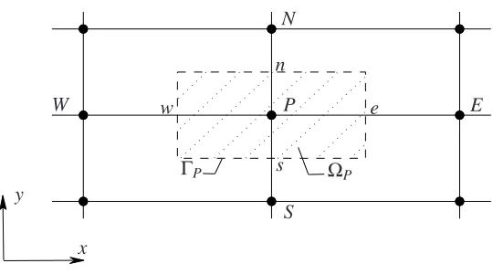
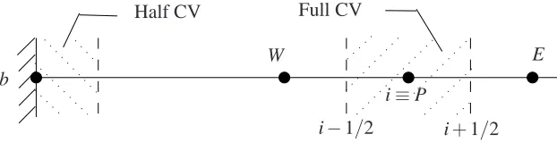
Assuming that a Cartesian-grid represents the problem domain Ω. In a control-volume approach, the domain is subdivided into a set of control control-volumes in such a way that there is one control volume surrounding each grid point without gaps or overlapped volumes between adjacent elements. A typical control volume asso-ciated with a grid point P, denoted byΩP, is shown in Fig. 2, where E,W,N and S are the neighbouring points of P on the horizontal and vertical grid lines. The

governing equation (8) is discretised by means of subregion collocation and this process is conducted in a similar fashion for all interior grid points of the problem domain.

By directly integrating (8) overΩP, the subregion-collocation equation is obtained

Z

ΩP

_∂2φ

∂x2 +

∂2φ

∂y2 −b(x,y)

dΩP=0. (21)

Applying the Gauss divergence theorem to (21) results in

Z

ΓP

_∂φ

∂xdy−

∂φ ∂ydx

−

Z

ΩP

whereΓP denotes the faces ofΩP. It is noted that partial derivatives of φ in (22) are of first order only and no approximation is made at this stage. Following the work of Patankar (1980), (22) reduces to

_∂φ ∂x e − _∂φ ∂x w

∆y+

_∂φ ∂y n − _∂φ ∂y s

∆x−b(xP,yP)AP=0, (23)

where AP is the area ofΩP and the subscripts e,w,n and s are used to indicate that the flux is estimated at the intersections of the grid lines with the east, west, north and south faces of the control volume, respectively (Fig. 2).

In the presently proposed technique, 2-node IRBFEs, which are defined over line segments between P and its neighbouring grid points (E,W,N and S), are

incor-porated into (23) to represent the field variableφ and its derivatives. There are 4 IRBFEs associated with a control volume. Assuming that PE and WP are interior elements and making use of (15), the values of the flux at the faces x=xe and

x=xware computed as

_∂φ

∂x

e

=hI₁(1)(xe),I(

1)

2 (xe),1,0 i

I−1ψ_b=h_I(1)

1 (xe),I(

1)

2 (xe),1,0 i

I−1      φP φE ∂φP ∂x ∂φE ∂x     

with η1≡xP and η2≡xE, (24)

_∂φ

∂x

w

=hI₁(1)(xw),I₂(1)(xw),1,0 i

I−1ψ_b=h_I(1)

1 (xw),I (1)

2 (xw),1,0

i I−1

     φW φP ∂φW ∂x ∂φP ∂x     

with η1≡xW and η2≡xP, (25)

where I₁(1)(x), I₂(1)(x)andI−1_{are defined in (9)-(13). Vector}ψ_{bmay change if PE}

and WP are semi-interior elements. For example, one has

b

ψ= (φW,φP,∂φP/∂x)T if WP is a D1 element, b

ψ= φW,∂2φW/∂x2,φP,∂φP/∂xT if WP is a D2 element, b

ψ= (φW,∂φW/∂x,φP,∂φP/∂x)T if WP is a D3 element, b

ψ= ∂φW/∂x,∂2φW/∂x2,φP,∂φP/∂x T

if WP is a N1 element, b

ψ= (φW,∂φW/∂x,φP,∂φP/∂x)T if WP is a N2 element.

3.4 Inter-element C2continuity

It can be seen from IRBFE expressions for computing the flux at the faces (e.g. (24) and (25)), there are three unknowns, namelyφ,∂φ/∂x and∂φ/∂y, at a grid node P.

Unlike conventional CVMs, the nodal values of∂φ/∂x and∂φ/∂y at P here

con-stitute part of the nodal unknown vector. One thus needs to generate three indepen-dent equations. The first equation is obtained by conducting subregion-collocation of (8) at P, i.e. (23). The other two equations can be formed by enforcing the local continuity of∂2φ/∂x2and∂2φ/∂y2across the elements at P

_∂2φ

P

∂x2

L

=

_∂2φ

P

∂x2

R

, (26)

_∂2φ

P

∂y2

B

=

_∂2φ

P

∂y2

T

, (27)

where(.)Lindicates that the computation of(.)is based on the element to the left of P, i.e. element WP, and similarly subscripts R,B,T denote the right (PE), bottom

(SP) and top (PN) elements.

Substitution of (16) into (26) and (27) yields h

I₁(2)(η2),I2(2)(η2),0,0

i

I−1ψ_b L=

h

I₁(2)(η1),I2(2)(η1),0,0

i

I−1ψ_b

R, (28) whereηrepresents x andη2≡η1≡xP, and

h

I₁(2)(η2),I2(2)(η2),0,0

i

I−1ψ_b B=

h

I₁(2)(η1),I2(2)(η1),0,0

i

I−1ψ_b

T, (29) where η represents y andη2 ≡η1 ≡yP. The conditions (26)-(27) or (28)-(29) guarantee that the solutionφ across IRBFEs is a C2function.

As discussed earlier, for IRBFE-D3, IRBFE-N1 and IRBFE-N2 elements, there is one unknown at a boundary node and one more extra equation needs be formed. This equation can be generated by integrating (8) over a half control-volume asso-ciated with that boundary node (Patankar (1980)).

Collection of the discretised equations at the appropriate nodal points and the con-tinuity equations at the interior grid points leads to a square system of algebraic equations that is sparse and banded. Two-point line elements are well suited to discretisation methods based on Cartesian grids.

4 Numerical results

length h by a factor β. The value of β is considered in a wide range from 1 to 85 to study its influence on the accuracy. In the case of non-rectangular domains, there may be some nodes that are too close to the boundary. If an interior node falls within a distance of h/2 to the boundary, such a node is removed from the set of nodal points.

The solution accuracy of an approximation scheme is measured by means of the discrete relative L2errors for the field variable and its first-order partial derivatives

Ne(φ) = r

∑M i=1

φ(e)

i −φi 2

r

∑M i=1

φ(e)

i

2 , (30)

Ne _∂φ ∂x = s ∑M i=1

∂φ(e)

i

∂x − ∂φi

∂x 2

s

∑M i=1

∂φ(e)

i

∂x

2 , (31)

Ne _∂φ ∂y = s ∑M i=1

∂φ(e)

i

∂y − ∂φi

∂y 2

s

∑M i=1

∂φ(e)

i

∂y

2 , (32)

where the superscript(e)refers to the exact solution and M is the length of a test set that is comprised of groups of 500 uniformly distributed points on grid lines. Another important measure is the convergence rate of the solution with respect to the refinement of spatial discretisation

Ne(h)≈γhα=O(hα), (33)

in whichα andγare exponential model’s parameters. Given a set of observations, these parameters can be found by the general linear least squares technique. To assess the performance of the proposed technique, the standard CVM (Patankar (1980)) is also implemented here.

4.1 Function approximation

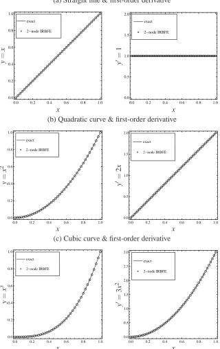
The present 2-node IRBFE scheme is first applied to the representation of func-tions. Consider four different test functions, namely straight line y=x, quadratic

domain of interest is[0,1]that is represented by one element only. Values of y and

dy/dx are given at x=0 and x=1. Fig. 3 shows the plots of the approximate

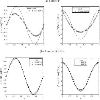
and exact functions for the first three cases where good agreement is achieved with only one element. It should be pointed out that, for the second and third functions, curved lines are reproduced even only two nodes (i.e. only one element) are em-ployed. The fourth function y=sin(2πx)is infinitely smooth and it is clear that one can construct several other approximate functions that would satisfy the four given input data. The present scheme picks up one of them, probably the simplest one (Fig. 4a). As more elements are used, a closer approximation to the exact function is obtained as shown in Fig. 4b. Numerical results for the last three functions show that the present two-node IRBFE has the ability to produce curved lines between its two extremes. This can be seen as a strength of IRBFEs over linear elements used in conventional techniques.

4.2 Solution of ODEs

4.2.1 Problem 1

Consider a 1D problem governed by

d dx

dφ dx

+φ+x=0, 0_≤x_≤1, (34)

and subject to two cases of boundary conditions

Case 1: φ(0) =0 andφ(1) =0 (Dirichlet boundary conditions only)

Case 2: φ(0) =0 and dφ(1)/dx=cot(1)₋1 (Dirichlet and Neumann boundary conditions).

The exact solution of this problem can be verified to be

φ(e)_{(x) =} sin(x)

sin(1)−x. (35)

The problem domain is discretised by n uniformly-distributed points. Each node xi is associated with a control volume denoted byΩi. For 2_≤i_≤n₋1,Ωiis defined as[xi−1/2,xi+1/2](full CV). For i=1 and i=n, Ωi is taken to be [x1,x1+1/2]and

Hereafter, Di-Dj is used to denote the boundary treatment strategy in which the boundary region[x1,x2]is represented by element IRBFE-Di and[xn−1,xn]by

IRBFE-Dj, while Di-Nj represents the strategy in which[x1,x2]and[xn₋1,xn]are modelled by elements IRBFE-Di and IRBFE-Nj, respectively. We employ the values of n ranging from 7 to 151 for h-adaptivity studies and the values ofβ from 1 to 85 for

β-adaptivity studies.

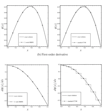
Case 1: Fig. 6 shows the plots ofφand dφ/dx by the proposed technique using the D1-D1 strategy and by the standard CVM. It can be seen that the present solution

is smooth for both φ and dφ/dx even with only a few interior nodes used. On

the other hand, using linear interpolations, the standard CV solution for dφ/dx has

a stair-case shape. To alleviate this zigzag variation, much more grid points are needed. Grid convergence studies for the proposed method employed with various values ofβand for the standard CVM are depicted in Fig. 7. It can be seen that the former outperforms the latter. At dense grids, in terms of the error Ne, the results for dφ/dx show a remarkable four orders of magnitude improvement (Fig. 7b).

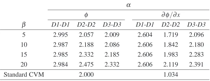
Fig. 8 and Tab. 2 compare the performance of the proposed method among three types of semi-interior element strategies, namely D1-D1, D2-D2 and D3-D3. Re-sults obtained by the standard CVM are also included and they are taken here as the reference. With more information incorporated into the IRBFE approximations, the D2-D2 and D3-D3 strategies yield much more accurate results than D1-D1, and

D3-D3 works better than D2-D2 as shown in Fig. 8a-b. Tab. 2 indicates that rates

obtained by the three strategies are generally higher than those by the standard CVM. For example, D1-D1 yields O(h2.99) forφ and O(h2.61) for dφ/dx, while

the standard CVM gives O(h2.00)forφ and O(h1.03)for dφ/dx. An improvement

in the approximation quality for dφ/dx is thus much bigger than that for φ. It should be noted that D1-D1 exhibits higher rates of grid convergence but produces less accurate results than D2-D2 and D3-D3.

In Fig. 9, the effects ofβ on the solution accuracy for coarse (n=9) and dense (n=153) grids are studied. Asβ increases, the overall error of the IRBFE solution is first reduced and then becomes flat/fluctuated. There are dramatic reductions (i.e. exponential convergence) in Ne(φ) and Ne(dφ/dx) for the D2-D2 and

D3-D3 strategies. In the case of large n and using D2-D2 and D3-D3-D3-D3, it appears that

there exists an optimal value forβ, e.g.β =42 for D2-D2 andβ =32 for D3-D3. Nevertheless, the present method can work with a wide range ofβ. This ability is also clearly seen in Fig. 7.

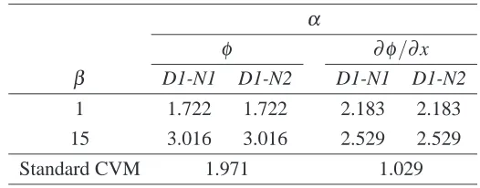
Case 2: Results obtained by the D1-N1 and D1-N2 strategies using β =1 and

of magnitude for dφ/dx. It is also observed that β can be used as an effective tool to enhance the solution accuracy. Tab. 3 shows that the present two schemes converge faster than the standard CVM. For example, the rates are O(h3.02) forφ and O(h2.53)for dφ/dx by the present two strategies (β =15), and O(h1.97)forφ and O(h1.03)for dφ/dx by the standard CVM.

4.2.2 Problem 2

In this example, the ODE involves more terms and its solution is highly oscillatory. The equation takes the form

d2φ

dx2 +

dφ

dx +φ=−e

−5x_{(9979 sin(100x) +900 cos(100x)), 0≤x≤1. (36)}

We consider two cases of boundary conditions: Dirichlet-Dirichlet (Case 1) and Dirichlet-Neumann (Case 2). The plots of the exact solutionφ(e)=sin(100x)e−5x

and its first-order derivative are shown in Fig. 11. Computations are conducted with the values of n varying from 23 to 403 and the values ofβ from 1 to 80. Re-sults concerning h adaptivity andβ adaptivity are presented in Fig. 12, Fig. 13 and Tab. 4 for Case 1, and in Fig. 14 and Tab. 5 for Case 2. Remarks here are similar to those in Problem 1. It should be pointed out that

(i) very high rates of grid convergence, i.e. up to O(h4.23)forφand O(h3.80)for dφ/dx

(Case 1), and O(h4.38)forφ and O(h3.92)for dφ/dx (Case 2), are achieved here,

(ii) the IRBFE solution is very stable (i.e. no fluctuation) at large values ofβ,

(iii) given a grid size h and a value ofβ, the overall errors for Case 2 are as low as those for Case 1,

(iv) the accuracy improvement is more significant for dφ/dx than forφ. This problem (Case 1) was also solved in Mai-Duy and Tran-Cong (2008) using the multidomain (MD) RBF collocation method. Two versions, namely differentiated-RBF (MD-Ddifferentiated-RBF) and integrated-differentiated-RBF (MD-Idifferentiated-RBF) schemes, were implemented. Using two non-overlapping subdomains,β=1 and 201 nodes/subdomain (i.e. 401 nodes for the whole domain), the obtained Neerrors forφ were 0.2 for MD-DRBF and 2.72×10−4 for MD-IRBF. Using the same set of nodes (i.e. 401 points or 400 IRBFEs), β =15 and D3-D3, the present method yields Ne =1.28_×10−5, which is much lower than those by the MD-RBF collocation method. It is noted that conventional/global RBF methods are able to work with low values ofβ such asβ=1.

4.3 Solution of PDEs

employed to deal with Dirichlet boundary conditions, while IRBFE-N2 is used for Neumann boundary conditions. It is noted that IRBFE-D1 can be applicable to problems with regular as well as irregular geometries. All IRBFE calculations here are carried out with two values ofβ, namely 1 and 15.

4.3.1 Problem 1: rectangular domain

Consider the following Poisson equation

∂2φ

∂x2 +

∂2φ

∂y2 =−2π

2_{cos(πx)cos(πy), (37)}

on a square domain 0_≤x,y_≤1 with two different cases of boundary conditions Case 1:

φ=cos(πy) for x=0,0_≤y_≤1

φ=₋cos(πy) for x=1,0_≤y_≤1

φ=cos(πx) for y=0,0≤x≤1

φ=₋cos(πx) for y=1,0_≤x_≤1

Case 2:

φ=cos(πy) for x=0,0≤y≤1

φ=₋cos(πy) for x=1,0_≤y_≤1

∂φ

∂y =0 for y=0,0≤x≤1

∂φ

∂y =0 for y=1,0≤x≤1.

The exact solution to this problem can be verified to be

φ(e)_{(x,y) =cos(πx)cos(πy). (38)}

line and hence the approximate solution φ is also C2-continuous on these lines. It can be seen that the size of the discretised system in Case 2 is slightly larger than that in Case 1.

To study the convergent behaviour of the proposed technique, various grids, namely (5_×5, 9_×9,..., 73_×73), are employed. Results concerning the relative L2 error

and the rate of convergence with grid refinement by the present and standard CV methods are shown in Fig. 16 for Case 1, Fig. 17 for Case 2, and Tab. 6 for Case 1 and Case 2.

It can be seen from Fig. 16 and Fig. 17, the present D1-D1, D2-D2 and D1-N2 strategies employed with a wide range ofβ produce much more accurate results especially for∂φ/∂x and∂φ/∂y than the standard CV method. For instance, at a

grid of 73_×73 andβ =15, the improvement is about one order of magnitude for the field variable and about three orders of of magnitude for its first-order partial derivatives. For Case 1 (Fig. 16), results at coarse grids by the D2-D2 strategy are a bit more accurate than those by D1-D1, probably owing to the fact that the former uses information about (37) on the boundary.

It can be seen from Tab. 6, the present method yields a faster convergence, espe-cially for∂φ/∂x and∂φ/∂y, than the standard CV method for both Case 1 and

Case 2. For example, in Case 1, the solutions∂φ/∂x and∂φ/∂y converge at the

rate O(h2.35)using the D1-D1 strategy, O(h2.10)using D2-D2, and O(h1.00)using the standard CV method.

Like in 1D problems, the use ofβ =15 (i.e. large values) here also leads to better accuracy and faster convergence especially for first-order partial derivatives than the use ofβ =1 (i.e. small values), and the IRBFE solutions for Case 1 and Case 2 have similar degrees of accuracy.

4.3.2 Problem 2: circular domain

Findφ such that

∂2_φ

∂x2 +

∂2_φ

∂y2 =0, (39)

on a circular domain of radiusπ/2 centred at (π/2,π/2) with Dirichlet boundary conditions. The exact solution to this problem is chosen to be

φ(e)_{(x,y) =} 1

sinh(π)sin(x)sinh(y), (40)

from which one can easily derive the boundary values ofφ.

employ semi-interior elements IRBFE-D1 for the handling of boundary conditions. Results obtained are presented in Fig. 19, which plots the solution accuracy Ne against the grid size h. It can be seen that the error is consistently reduced as a grid is refined.

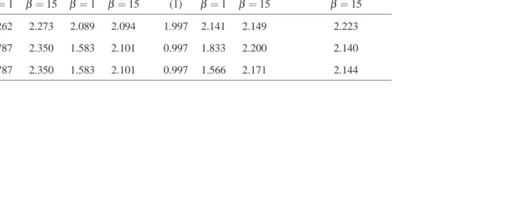
Tab. 6 also compares the rate of convergence by the proposed technique between Problem 1 (rectangular domain) and Problem 2 (circular domain). Using the same

D1-D1 strategy andβ =15, the orders of accuracy of the solutions φ,∂φ/∂x and

∂φ/∂y for the two types of domains are all greater than 2. It can be seen that the

proposed technique is able to work well not only for rectangular domains but also for non-rectangular domains.

5 Concluding remarks

In this paper, a new Cartesian-grid-based control-volume technique is proposed for the solution of second-order elliptic problems in one and two dimensions. In-tegrated RBFs are utilised to construct the approximations for the field variable and its derivatives, which are based on two-node elements and expressed in terms of nodal values of the field variable and its first-order partial derivatives. Various strategies for the imposition of boundary conditions are presented. The proposed control-volume method leads to a system matrix that is sparse and produces a solu-tion that is C2-continuous on the grid lines. Its solution accuracy can be effectively controlled by means of the shape parameter (β up to 85) and/or grid size. A series of test problems including those defined on non-rectangular domains are employed to validate the present method. Numerical results show that the method is much more accurate and faster convergence, especially for the approximation of deriva-tives, than the standard control volume method.

Acknowledgement: D.-A. An-Vo would like to thank USQ, FoES and CESRC for a PhD scholarship. This research is supported by the Australian Research Coun-cil.

References

Atluri, S. N.; Han, Z. D.; Rajendran, A. M. (2004): A new implementation of the meshless finite volume method, through the MLPG “mixed” approach. CMES:

Computer Modeling in Engineering and Sciences, vol. 6, pp. 491–514.

Divo, E.; Kassab, A. J. (2007): An efficient localized radial basis function mesh-less method for fluid flow and conjugate heat transfer. Journal of Heat Transfer, vol. 129, pp. 124–136.

Fasshauer, G. E. (2007): Meshfree approximation methods with Matlab.

Inter-disciplinary mathematical sciences, vol. 6. Singapore: World Scientific Publishers.

Fedoseyev, A. I.; Friedman, M. J.; Kansa, E. J. (2002): Improved multiquadric method for elliptic partial differential equations via PDE collocation on the bound-ary. Computers and Mathematics with Applications, vol. 43, pp. 439–455.

Franke, R. (1982): Scattered data interpolation: tests of some methods.

Mathe-matics of Computation, vol. 38, pp. 182–200.

Ho-Minh, D.; Mai-Duy, N.; Tran-Cong, T. (2009): A Galerkin-RBF approach for the streamfunction-vorticity-temperature formulation of natural convection in 2D enclosured domains. CMES: Computer Modeling in Engineering and Sciences, vol. 44, pp. 219–248.

Kansa, E. J. (1990): Multiquadrics-a scattered data approximation scheme with applications to computational fluid-dynamics-II. Computers and Mathematics with

Applications, vol. 19, pp. 147–161.

Le-Cao, K.; Mai-Duy, N.; Tran-Cong, T. (2009): An effective intergrated-RBFN Cartesian-grid discretization for the stream function-vorticity-temperature formula-tion in nonrectangular domains. Numerical Heat Transfer, Part B: Fundamentals, vol. 55, pp. 480 – 502.

Lee, C. K.; Liu, X.; Fan, S. C. (2003): Local multiquadric approximation for solving boundary value problems. Computational Mechanics, vol. 30, pp. 396–

409.

Li, J.; Hon, Y. C. (2004): Domain decomposition for radial basis meshless methods. Numerical Methods for Partial Differential Equations, vol. 20, pp. 450– 462.

Libre, N. A.; Emdadi, A.; Kansa, E. J.; Rahimian, M.; Shekarchi, M. (2008): A stabilized RBF collocation scheme for Neumann type boundary value problems.

CMES: Computer Modeling in Engineering and Sciences, vol. 24, pp. 61–80.

Madych, W. R. (1992): Miscellaneous error bounds for multiquadric and related interpolators. Computers and Mathematics with Applications, vol. 24, pp. 121–

Mai-Duy, N.; Le-Cao, K.; Tran-Cong, T. (2008): A Cartesian grid technique based on one-dimensional integrated radial basis function networks for natural con-vection in concentric annuli. International Journal for Numerical Methods in

Flu-ids, vol. 57, pp. 1709–1730.

Mai-Duy, N.; Tran-Cong, T. (2001): Numerical solution of differential equations using multiquadric radial basis function networks. Neural Networks, vol. 14, pp. 185–199.

Mai-Duy, N.; Tran-Cong, T. (2003): Approximation of function and its deriva-tives using radial basis function network methods. Applied Mathematical Mod-elling, vol. 27, pp. 197–220.

Mai-Duy, N.; Tran-Cong, T. (2007): A Cartesian-grid collocation method based on radial-basis-function networks for solving PDEs in irregular domains.

Numeri-cal Methods for Partial Differential Equations, vol. 23, pp. 1192–1210.

Mai-Duy, N.; Tran-Cong, T. (2008): A multidomain integrated-radial-basis-function collocation method for elliptic problems. Numerical Methods for Partial

Differential Equations, vol. 24, pp. 1301–1320.

Mai-Duy, N.; Tran-Cong, T. (2009): A Cartesian-grid discretisation scheme based on local integrated RBFNs for two-dimensional elliptic problems. CMES:

Computer Modeling in Engineering and Sciences, vol. 51, pp. 213–238.

Mai-Duy, N.; Tran-Cong, T. (2010): A control volume technique based on integrated RBFNs for the convection-diffusion equation. Numerical Methods for

Partial Differential Equations, vol. 26, pp. 426–447.

Mohammadi, M. H. (2008): Stabilized meshless local Petrov-Galerkin (MLPG) method for incompressible viscous fluid flows. CMES: Computer Modeling in Engineering and Sciences, vol. 29, pp. 75–94.

Ngo-Cong, D.; Mai-Duy, N.; Karunasena, W.; Tran-Cong, T. (2011): Free vibration analysis of laminated composite plates based on FSDT using one-dimensional IRBFN method. Computers and Structures, vol. 89, pp. 1–13.

Orsini, P.; Power, H.; Morvan, H. (2008): Improving volume element meth-ods by meshless radial basis function techniques. CMES: Computer Modeling in

Engineering and Sciences, vol. 23, pp. 187–208.

Sanyasiraju, Y. V. S. S.; Chandhini, G. (2008): Local radial basis function based gridfree scheme for unsteady incompressible viscous flows. Journal of

Computa-tional Physics, vol. 227, pp. 8922–8948.

Sarler, B. (2005): A radial basis function collocation approach in computational fluid dynamics. CMES: Computer Modeling in Engineering and Sciences, vol. 7, pp. 185–194.

Sellountos, E. J.; Sequeira, A. (2008): A hydrid multi-region BEM/LBIE-RBF velocity-vorticity scheme for the two-dimensional Navier-Stokes equations.

CMES: Computer Modeling in Engineering and Sciences, vol. 23, pp. 127–148.

Shu, C.; Ding, H.; Yeo, K. S. (2003): Local radial basis function-based differen-tial quadrature method and its application to solve two-dimensional incompressible Navier-Stokes equations. Computer Methods in Applied Mechanics and

Engineer-ing, vol. 192, pp. 941–954.

Tolstykh, A. I.; Shirobokov, D. A. (2003): On using radial basis functions in “finite difference mode” with applications to elasticity problems. Computational

Mechanics, vol. 33, pp. 68–79.

Šarler, B.; Vertnik, R. (2006): Meshfree explicit local radial basis function collocation method for diffusion problems. Computers and Mathematics with

Ap-plications, vol. 51, pp. 1269–1282.

Zerroukat, M.; Power, H.; Chen, C. S. (1998): A numerical method for heat transfer probems using collocation and radial basis functions. International

Table 1: List of semi-interior elements and their characteristics.

Boundary condition Element Nodal values at a boundary point Unknowns

Dirichlet IRBFE-D1 φb None

IRBFE-D2 φband∂2φb/∂η2 None

IRBFE-D3 φband∂φb/∂η ∂φb/∂η

Neumann IRBFE-N1 ∂φb/∂ηand∂2φb/∂η2 ∂2φb/∂η2

IRBFE-N2 φband∂φb/∂η φb

Table 2: ODE, Problem 1, Dirichlet boundary conditions: rates of convergence

O(hα)forφand∂φ/∂x for several largeβ values and semi-interior element types.

α

φ ∂φ/∂x

β D1-D1 D2-D2 D3-D3 D1-D1 D2-D2 D3-D3

5 2.995 2.057 2.009 2.604 1.719 2.096

10 2.987 2.188 2.086 2.606 1.842 2.180

15 2.985 2.332 2.185 2.606 1.983 2.283

20 2.984 2.475 2.332 2.606 2.119 2.391

Table 3: ODE, Problem 1, Dirichlet-Neumann boundary conditions: rates of con-vergence O(hα)forφand∂φ/∂x for two semi-interior element types.

α

φ ∂φ/∂x

β D1-N1 D1-N2 D1-N1 D1-N2

1 1.722 1.722 2.183 2.183

15 3.016 3.016 2.529 2.529

Standard CVM 1.971 1.029

Table 4: ODE, Problem 2, Dirichlet boundary conditions: rates of convergence

O(hα)forφ and∂φ/∂x for severalβ values and semi-interior element types.

α

φ ∂φ/∂x

Boundary treatment β =1 β =15 β =1 β =15

D1-D1 2.540 2.582 2.554 2.670

D2-D2 2.679 3.965 2.713 3.932

D3-D3 2.971 4.229 2.588 3.801

Standard CVM 2.194 0.971

Table 5: ODE, Problem 2, Dirichlet and Neumann boundary conditions, D3-N2 treatment: rates of convergence O(hα)forφand∂φ/∂x for severalβ values.

α

β φ ∂φ/∂x

1 3.240 2.706

15 4.380 3.919

2

4

derivatives, (1): standard CVM.

α

Problem 1 Problem 2

(Rectangular domain) (Circular domain)

Dirichlet Dirichlet & Neumann Dirichlet

D1-D1 D2-D2 D1-N2 D1-D1

(1) β=1 β=15 β =1 β =15 (1) β =1 β =15 β=15

φ 1.997 2.262 2.273 2.089 2.094 1.997 2.141 2.149 2.223

∂φ/∂x 0.997 1.787 2.350 1.583 2.101 0.997 1.833 2.200 2.140

η

φ1 φ2

∂φ1

∂η ∂φ∂η2

Figure 1: Schematic outline for 2-node IRBFE.

x y

ΓP ΩP

N

S

W P E

n

s

e w

(a) Straight line & first-order derivative

0.0 0.2 0.4 0.6 0.8 1.0

0.0 0.2 0.4 0.6 0.8 1.0 2

-node IRBFE

exact

x

y

=

x

0.0 0.2 0.4 0.6 0.8 1.0

0.0 0.5 1.0 1.5 2.0 2

-node IRBFE

exact

x

y

′ =

1

(b) Quadratic curve & first-order derivative

0.0 0.2 0.4 0.6 0.8 1.0

0.0 0.2 0.4 0.6 0.8 1.0

2-node IRBFE

exact x y = x 2

0.0 0.2 0.4 0.6 0.8 1.0

0.0 0.5 1.0 1.5 2.0

2_-node IRBFE exact x y ′ = 2 x

(c) Cubic curve & first-order derivative

0.0 0.2 0.4 0.6 0.8 1.0

0.0 0.2 0.4 0.6 0.8 1.0

2-node IRBFE

exact x y = x 3

0.0 0.2 0.4 0.6 0.8 1.0

0.0 0.5 1.0 1.5 2.0 2.5 3.0

2_-node IRBFE exact x y ′ = 3 x 2

(a) 1 IRBFE

0 0.2 0.4 0.6 0.8 1

−1 −0.8 −0.6 −0.4 −0.2 0 0.2 0.4 0.6 0.8 1 exact 2−node IRBFE x y = si n ( 2 π x )

0 0.2 0.4 0.6 0.8 1

−8 −6 −4 −2 0 2 4 6 8 exact 2−node IRBFE x y ′ = 2 π co s ( 2 π x )

(b) 3 and 4 IRBFEs

0 0.2 0.4 0.6 0.8 1

−1 −0.8 −0.6 −0.4 −0.2 0 0.2 0.4 0.6 0.8 1 exact 3 IRBFEs 4 IRBFEs x y = si n ( 2 π x )

0 0.2 0.4 0.6 0.8 1

−8 −6 −4 −2 0 2 4 6 8 exact 3 IRBFEs 4 IRBFEs x y ′ = 2 π co s ( 2 π x )

b

W E

i_≡P

i₋1/2 i+1/2

Full CV Half CV

(a) Field variable

0.0 0.2 0.4 0.6 0.8 1.0

0.00 0.01 0.02 0.03 0.04 0.05 0.06 0.07

2_-node IRBFE exact solution

x

φ

(

x

)

0.0 0.2 0.4 0.6 0.8 1.0

0.00 0.01 0.02 0.03 0.04 0.05 0.06 0.07

standard CVM exact solution

x

φ

(

x

)

(b) First-order derivative

0.0 0.2 0.4 0.6 0.8 1.0

-0.3 -0.2 -0.1

0.0 0.1 0.2

2_-node IRBFE exact solution

x

d

φ

(

x

)

/

d

x

0.0 0.2 0.4 0.6 0.8 1.0

-0.3 -0.2 -0.1

0.0 0.1 0.2

standard CVM exact solution

x

d

φ

(

x

)

/

d

x

(a) Field variable (b) First-order derivative 10−3 10−2 10−1 100 10−7 10−6 10−5 10−4 10−3 β=1 β=5 β=10 β=15 standard CVM h Ne ( φ ) 10−3 10−2 10−1 100 10−6 10−5 10−4 10−3 10−2 10−1 100 β=1 β=5 β=10 β=15 standard CVM h Ne d φ _dx

Figure 7: ODE, Problem 1, Dirichlet boundary conditions: h-adaptivity studies conducted with several values ofβ for the D1-D1 strategy. It is noted that results withβ = (5,10,15) are undistinguishable.

(a) Field variable (b) First-order derivative

10−3 10−2 10−1 100

10−9 10−8 10−7 10−6 10−5 10−4 10−3 D1−D1 D2−D2 D3−D3 standard CVM h Ne ( φ )

10−3 10−2 10−1 100

10−9 10−8 10−7 10−6 10−5 10−4 10−3 10−2 10−1 100 D1−D1 D2−D2 D3−D3 standard CVM h Ne d φ _dx

(a) Field variable

0 10 20 30 40 50 60 70 80 90 10−7

10−6 10−5 10−4 10−3 10−2

D1−D1 D2−D2 D3−D3

β

Ne

(

φ

)

0 10 20 30 40 50 60 70 80 90 10−10

10−9 10−8 10−7 10−6 10−5

D1−D1 D2−D2 D3−D3

β

Ne

(

φ

)

(b) First-order derivative

0 10 20 30 40 50 60 70 80 90 10−5

10−4 10−3 10−2

D1−D1 D2−D2 D3−D3

β

Ne

d φ _dx

0 10 20 30 40 50 60 70 80 90 10−9

10−8 10−7 10−6 10−5

D1−D1 D2−D2 D3−D3

β

Ne

d φ _dx

(a) Field variable

10−3

10−2

10−1

100 10−7

10−6 10−5 10−4 10−3 10−2

D1−N1 D1−N2 standard CVM

h

Ne

(

φ

)

10−3

10−2

10−1

100 10−7

10−6 10−5 10−4 10−3 10−2

D1−N1 D1−N2 standard CVM

h

Ne

(

φ

)

(b) First-order derivative

10−3 ₁₀−2 ₁₀−1 ₁₀0

10−8 10−6 10−4 10−2 100

D1−N1 D1−N2 standard CVM

h

Ne

d φ _dx

10−3 10−2 10−1 100

10−8 10−6 10−4 10−2 100

D1−N1 D1−N2 standard CVM

h

Ne

d φ _dx

(a) (b)

0 0.2 0.4 0.6 0.8 1

−1 −0.8 −0.6 −0.4 −0.2 0 0.2 0.4 0.6 0.8 1

x

ue

0 0.2 0.4 0.6 0.8 1 −100

−50 0 50 100

x

u

, e

(a) Field variable

10−3 10−2 10−1

10−5 10−4 10−3 10−2 10−1 100 101

D1−D1 D2−D2 D3−D3 standard CVM

h

Ne

(

φ

)

10−3 10−2 10−1

10−5 10−4 10−3 10−2 10−1 100 101

D1−D1 D2−D2 D3−D3 standard CVM

h

Ne

(

φ

)

(b) First-order derivative

10−3 10−2 10−1

10−5 10−4 10−3 10−2 10−1 100 101

D1−D1 D2−D2 D3−D3 standard CVM

h

Ne

d φ _dx

10−3 10−2 10−1

10−5 10−4 10−3 10−2 10−1 100 101

D1−D1 D2−D2 D3−D3 standard CVM

h

Ne

d φ _dx

(a) Field variable

0 10 20 30 40 50 60 70 80 90 10−3

10−2

10−1

D1−D1 D2−D2 D3−D3

β

Ne

(

φ

)

0 10 20 30 40 50 60 70 80 90 10−5

10−4 10−3 10−2

D1−D1 D2−D2 D3−D3

β

Ne

(

φ

)

(b) First-order derivative

0 10 20 30 40 50 60 70 80 90 10−3

10−2 10−1

D1−D1 D2−D2 D3−D3

β

Ne

d φ _dx

0 10 20 30 40 50 60 70 80 90 10−5

10−4

10−3

10−2

D1−D1 D2−D2 D3−D3

β

Ne

d φ _dx

(a) Field variable

10−3 10−2 10−1

10−5 10−4 10−3 10−2 10−1 100 101

β=1 β=15 standard CVM

h

Ne

(

φ

)

0 10 20 30 40 50 60 70 80 90 10−5

10−4

10−3

10−2 10−1

n=103 n=263 n=383

β

Ne

(

φ

)

(b) First-order derivative

10−3 10−2 10−1

10−5 10−4 10−3 10−2 10−1 100 101

β=1 β=15 standard CVM

h

Ne

d φ _dx

0 10 20 30 40 50 60 70 80 90 10−5

10−4 10−3 10−2

10−1

n=103 n=263 n=383

β

Ne

d φ _dx

N

W P E

Neumann Boundary Half CV

(a) Field variable

10−2 10−1 100

10−5 10−4 10−3 10−2 10−1 standard CVM D1−D1 (β=1) D1−D1 (β=15)

h

Ne

(

φ

)

10−2 10−1 100

10−5 10−4 10−3 10−2 10−1 standard CVM D2−D2 (β=1) D2−D2 (β=15)

h

Ne

(

φ

)

(b) First-order derivative with respect to x

10−2 10−1 100

10−5 10−4 10−3 10−2 10−1 100 standard CVM D1−D1 (β=1) D1−D1 (β=15)

h

Ne

∂φ ∂

x

10−2 10−1 100

10−5 10−4 10−3 10−2 10−1 100 standard CVM D2−D2 (β=1) D2−D2 (β=15)

h

Ne

∂φ ∂

x

(c) First-order derivative with respect to y

10−2 10−1 100

10−5 10−4 10−3 10−2 10−1 100 standard CVM D1−D1 (β=1) D1−D1 (β=15)

h

Ne

∂φ ∂

y

10−2 10−1 100

10−5 10−4 10−3 10−2 10−1 100 standard CVM D2−D2 (β=1) D2−D2 (β=15)

h

Ne

∂φ ∂

y

(a) Field variable

10−2 10−1 100

10−5 10−4 10−3 10−2 10−1

standard CVM D1−N2 (β=1) D1−N2 (β=15)

h

Ne

(

φ

)

(b) First-order derivative with respect to x

10−2 10−1 100

10−5 10−4 10−3 10−2 10−1 100

standard CVM D1−N2 (β=1) D1−N2 (β=15)

h

Ne

∂φ ∂

x

(c) First-order derivative with respect to y

10−2 10−1 100

10−5 10−4 10−3 10−2 10−1 100

standard CVM D1−N2 (β=1) D1−N2 (β=15)

h

Ne

∂φ ∂

y

0.0 0.5 1.0 1.5 2.0 2.5 3.0 0.0

0.5 1.0 1.5 2.0 2.5 3.0

x

y

10−2 10−1 100

10−5

10−4

10−3

10−2

10−1

Ne(φ)

Ne(dφ/dx)

Ne(dφ/dy)

h

Ne