A numerical scheme based on local integrated RBFNs and Cartesian grids for solving second-order elliptic problems in two dimensions

solving second-order elliptic problems in two dimensions

N. Mai-Duy1and T. Tran-Cong1

Abstract: This paper reports a new Cartesian-grid computational technique, based on local integrated radial-basis-function networks (IRBFNs), for the solution of second-order elliptic differential problems defined on two-dimensional regular and irregular domains. At each grid point, only neighbouring nodes are activated to construct the IRBFN approximations. Local IRBFNs are introduced into two different schemes for discretisa-tion of partial differential equadiscretisa-tions, namely point collocadiscretisa-tion and control-volume (CV)/subregion-collocadiscretisa-tion. Numerical experiments indicate that the latter outperforms the former regarding accuracy. Moreover, the pro-posed local IRBFN CV method shows a similar level of the matrix condition number and a significant improve-ment in accuracy over a linear CV method.

Keywords: local approximations, integrated RBFNs, point collocation, subregion collocation, second-order differential problems.

1 Introduction

RBF-based discretisation methods have emerged as a new attractive solver for partial differential equations (PDEs). They have the capability to work well for problems defined on irregular domains. Very accurate results can be achieved using only a relatively-small number of nodes. However, RBF matrices are dense and generally ill-conditioned. To resolve this problem, local RBF methods have been developed, resulting in having to solve a sparse system of algebraic equations. The RBF approximations are constructed locally on small overlapping regions which are represented by a set of structured points or a set of scattered points. Works reported include [Lee, Liu, and Fan (2003); Shu, Ding, and Yeo (2003); Wright and Fornberg (2006); Kosec and Sarler (2008); Sanyasiraju and Chandhini (2008)].

To transform a PDE into a set of algebraic equations, one needs to discretise the problem domain. For irregular domain, this task can be expensive and time-consuming. It can be seen that using Cartesian grids to represent the domain is economical. Considerable effort has been put into the development of Cartesian-grid-based computational techniques.

The proposed numerical procedure combines strengths of the local RBF approach and the Cartesian-grid ap-proach for solving 2D differential problems. At each grid point, only neighbouring nodes are activated to

con-1_{Computational Engineering and Science Research Centre, Faculty of Engineering and Surveying, University of Southern Queensland,}

struct the RBF approximations. Unlike local RBF techniques reported in the literature, RBFNs are employed here to approximate highest-order derivatives in a given PDE and subsequently integrated to obtain expressions for lower-order derivatives and the field variable. This use of integration to construct the approximations pro-vides an effective way to circumvent the problem of reduced convergence rate caused by differentiation and to implement derivative boundary conditions. In this study, we introduce local integrated RBFNs into two PDE discretisation formulations, namely point collocation and control-volume (CV)/subregion-collocation, and then conduct some numerical experiments to investigate accuracy of the two local IRBFN techniques.

The remainder of this paper is organised as follows. A brief review of integrated RBFNs is given in Section 2. The proposed computational procedure is presented in Section 3 and numerically verified through a series of examples in Section 4. Section 5 concludes the paper.

2 Integrated radial-basis-function networks

RBFNs allow a conversion of a function f from a low-dimensional space (e.g. 1D-3D) to a high-dimensional space in which the function can be expressed as a linear combination of RBFs

f(x) =

m

∑

i=1

w(i)G(i)(x), (1)

where the superscript (i)is the summation index, x the input vector, m the number of RBFs,_{w(i)_}m_i=1the set of network weights to be found, and_{G(i)(x)_}m

i=1the set of RBFs.

This study is concerned with second-order differential problems in two dimensions. The integral approach uses RBFNs (1) to represent the second-order derivatives of the field variable u in a given PDE. Approximate expressions for the first-order derivatives and the variable itself are then obtained through integration as

∂2_u(x)

∂x2_j =

m

∑

i=1

w(_[xji)_]G(i)(x), (2)

∂u(x)

∂xj

=

m

∑

i=1

w(_[xji)_]H_[(_xji)_](x) +C1[xj](xk), (3)

u[xj](x) = m

∑

i=1

w(_[xji)_]H(_[xi)

j](x) +xjC1[xj](xk) +C2[xj](xk), (4)

where the subscript[xj]is used to denote the quantities associated with the process of integration with respect

to the xj variable; C1[xj](xk) and C2[xj](xk) the constants of integration which are univariate functions of the

variable other than xj (i.e. xk with k6= j); H_[(_xji)_](x) =RG(i)(x)dxj and H( i) [xj](x) =

R

H_[(_xji)_](x)dxj. The reader is

referred to [Mai-Duy and Tanner (2005); Mai-Duy and Tran-Cong (2005)] for further details.

3 Proposed technique

using (2)-(4): one associated with the x1coordinate and the other with the x2coordinate. The two networks are

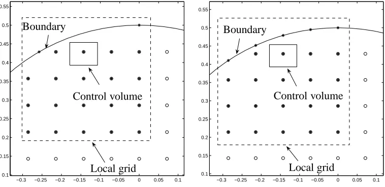
constructed on the same set of l×l grid lines. The reference point may not be the centre of the local grid when

the construction process is carried out near the boundary (Figure 1). For local grids entirely embedded in the

−0.3 −0.25 −0.2 −0.15 −0.1 −0.05 0 0.05 0.1

0.1 0.15 0.2 0.25 0.3 0.35 0.4 0.45 0.5 0.55

Local grid Control volume Boundary

−0.3 −0.25 −0.2 −0.15 −0.1 −0.05 0 0.05 0.1

0.1 0.15 0.2 0.25 0.3 0.35 0.4 0.45 0.5 0.55

Local grid Control volume Boundary

Figure 1: Local networks in x1(left) and x2(right) (∗: RBF centre and o: interior point).

domain, the two networks have the same set of RBF centres which are chosen to be the interior grid nodes. The value of m in (4) is equal to l2.

For local grids that are cut by irregular boundary, one generally has different sets of RBF centres for the two associated networks. A set of the RBF centres for the xj network is comprised of the interior grid nodes and

the boundary nodes generated by the xj grid lines. The value of m in (4) may be less than l2(Figure 1).

We also employ IRBFNs to represent the variation of the constants of integration. The construction process for

C1[xj](xk)is exactly the same as that for C2[xj](xk). To simplify the notation, some subscripts are dropped. The

function C(xk)is constructed through

d2C(xk)

dx2 k

=

l

∑

i=1

w(i)g(i)(xk), (5)

dC(xk)

dxk

=

l

∑

i=1

w(i)h(i)(xk) +c1, (6)

C(xk) =

l

∑

i=1

w(i)¯h(i)(xk) +xkc1+c2, (7)

where c1 and c2 are the constants of integration which are simply unknown values, and g(i), h(i) and ¯h(i) the

i=_{1,2,_···,l_}leads to b

C=Tc_{wb, (8)}

whereC andb w are the vectors of length l and_b (l+2), respectively, and Tc_{is the transformation matrix of}

dimensions l_×(l+2)

b

C=C(x(_k1)),C(x(_k2)),_···,C(x(_kl))T=C(1),C(2),_···,C(l) T

,

b

w=w(1),w(2),_···,w(l),c1,c2

T , c T ₌      

¯h(1)_(x(1)

k ), ¯h( 2)_(x(1)

k ), ···, ¯h( l)_(x(1)

k ), x

(1)

k , 1

¯h(1)_(x(2)

k ), ¯h(2)(x

(2)

k ), ···, ¯h(l)(x

(2)

k ), x

(2)

k , 1

..

. ... . .. ... ... ...

¯h(1)_(x(l)

k ), ¯h(2)(x

(l)

k ), ···, ¯h(l)(x

(l)

k ), x

(l)

k , 1

     .

Taking (8) into account, the value of C in (7) at an arbitrary point xk can be computed in terms of nodal values

of C as

C(xk) =

h ¯h(1)_(x

k),¯h(2)(xk),···,¯h(l)(xk),xk,1

i c

T+_Cb_{, (9)}

or

C(xk) = l

∑

i=1

P(i)(xk)C(i), (10)

where P(i)(xk)is the product of the first vector on RHS and the ith column ofTc+, andTc+is the generalised

inverse ofTc_.

Substitution of (10) into (3) and (4) yields

∂u(x)

∂xj

=

m

∑

i=1

w_[(_xji)_]H_[(_xji)_](x) +

l

∑

i=1

P_[(_xji)_](xk)C(₁i_[)_xj], (11)

u_[xj](x) =

m

∑

i=1

w(_[xji)_]H(_[xi)

j](x) + l

∑

i=1

xjP_[(_xji)_](xk)C(₁i_[)_xj]+ l

∑

i=1

P_[(_xi)

j](xk)C

(i)

2[xj]. (12)

For convenience of presentation, expressions (2), (11) and (12) can be rewritten as

∂2_u(x)

∂x2_j =

m+2l

∑

i=1

w(_[xji)_]G(_[xi)

j](x), (13)

∂u(x)

∂xj

=

m+2l

∑

i=1

w_[(_xji)_]H_[(_xji)_](x), (14)

u[xj](x) = m+2l

∑

i=1

w(_[xji)_]H(_[xi)

where

{G(_[xi)

j](x)} m+2l

i=m+1≡ {0} 2l i=1, {H_[(_xji)_](x)_}m+l

i=m+1≡ {P

(i) [xj](xk)}

l

i=1, {H

(i) [xj](x)}

m+2l

i=m+l+1≡ {0}li=1, {H(_[xi)

j](x)} m+l

i=m+1≡ {xjP_[(_xji)_](xk)}li=1, {H

(i) [xj](x)}

m+2l

i=m+l+1≡ {P

(i) [xj](xk)}

l i=1, {w(_[xi)

j]} m+l

i=m+1≡ {C

(i)

1[xj]} l

i=1,and{w

(i) [xj]}

m+2l

i=m+l+1≡ {C

(i)

2[xj]} l i=1.

We seek the solution in terms of nodal values of the field variable u. To do so, (15) is collocated at the nodal points on the local grid, from which the relationship between the network-weight space and the physical space can be established as

e

u[xj] = Tf[xj]we[xj], (16)

e

w_[xj] = Tf+

[xj]ue[xj], (17)

whereu_e[xj] is the vector of length m consisting of the nodal values of u on the local grid, we[xj] the vector of

length(m+2l)made up of the RBF weights and the nodal values of C₁(i_[)_xj]and C₂(i_[)_x

j], and f T+

[xj]the generalised

inverse of Tf

[xj]. The transformation matrix Tf[xj] has the entries Tf[xj]rs=H

(s)

[xj](x(r)), where 1≤r ≤m and 1_≤s_≤(m+2l).

It is noted that the two vectors,ue[x1]andue[x2], are unknown. From now on, they are forced to be identical

e

u[x1]≡ue[x2]≡ue. (18)

The values of u,∂u/∂xjand∂2u/∂x2j at an arbitrary point x can be computed in terms of nodal variable values

as

u(x) =1

2

2

∑

j=1

u[xj](x) = 1 2

2

∑

j=1

h

H_[(_xj1)_](x),H_[(_xj2)_](x),_···,H(_[xm+2l)

j] (x)

i f

T+

[xj]

e

u, (19)

∂u(x)

∂xj

=hH_[(_xj1)_](x),H_[(_xj2)_](x),_···,H_[(_xm+2l)

j] (x)

i f

T+

[xj]eu, (20)

∂2_u(x)

∂x2

j

=hG(1)(x),G(2)(x),_···,G(m+2l)(x)iTf+

[xj]ue, (21)

where the function value is computed in an average sense due to numerical error.

For the point-collocation formulation, there are no integrations required for the discretisation. The process of converting the PDE into a set of algebraic equations is straightforward.

through the middle points between the reference node and its neighbours/appropriate points on the boundary (Figure 1). Integrals can be calculated using Gauss quadrature since the present approximation scheme allows the accurate evaluation of the variable u and its derivatives at any point within the local grid.

The use of local integrated networks results in a sparse system of simultaneous equations. It can be seen that operations on zero elements are unnecessary. Avoiding these operations provides a considerable saving in time. By taking account of sparseness of the system matrix, one has the capability to reduce the computational time and storage facilities. Such sparse equation sets can be solved effectively by means of iterative solvers.

4 Numerical examples

For all numerical examples presented here, the approximations are constructed on local grids of 5_×5. IRBFNs are implemented with the multiquadric (MQ) basis function whose form is given

G(i)(x) =

q

(x₋c(i)₎T_(x−c(i)_{) +a}(i)2_{, (22)}

where c(i)and a(i)are the centre and width of the ith MQ basis function, respectively. The set of centres and the set of collocation points are identical. All MQ centres are associated with the same width that is chosen to be the grid size. We use the discrete relative L2 norm of u, denoted by Ne(u), to measure accuracy of an

approximate scheme. We apply the matrix 1-norm estimation algorithm for estimating condition numbers of the system matrix. Furthermore, linear CV (central difference) techniques, which are similar to those described in [Patankar (1980)], are referred to as a standard CV technique.

4.1 Test problem

Consider the following PDE

∂2_u

∂x2

1

+∂

2_u

∂x2

2

=0 (23)

with Dirichlet boundary conditions. Two computational domains, namely a unit square 0_≤x1,x2≤1 and a

circle centered at the origin with radius of 0.5, are considered. The exact solution is given by

ue=

1

sinh(π)sin(πx1)sin(πx2) (24)

from which the boundary values of u can be derived. The point-collocation formulation consists in forcing (23) to be satisfied exactly at discrete points in order to form a determined set of algebraic equations. It means that (23) needs be collocated at the interior grid nodes.

For the control-volume formulation, (23) is forced to be satisfied in the mean. Integrating (23) over a control volumeΩi, we have

Z

Ωi∇

2_udΩ

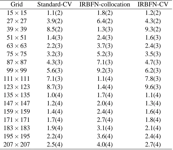
Table 1: Rectangular domain: Condition numbers of the system matrix by standard CV, local IRBFN colloca-tion and local IRBFN CV methods. Notice that a(b)means a_×10b.

Grid Standard-CV IRBFN-collocation IRBFN-CV

15_×15 1.1(2) 1.8(2) 1.2(2)

27_×27 3.9(2) 6.4(2) 4.3(2)

39_×39 8.5(2) 1.3(3) 9.3(2)

51×51 1.4(3) 2.4(3) 1.6(3)

63_×63 2.2(3) 3.7(3) 2.4(3)

75_×75 3.2(3) 5.2(3) 3.5(3)

87×87 4.3(3) 7.1(3) 4.7(3)

99_×99 5.6(3) 9.2(3) 6.2(3)

111_×111 7.1(3) 1.1(4) 7.8(3)

123×123 8.7(3) 1.4(4) 9.6(3)

135_×135 1.0(4) 1.7(4) 1.1(4)

147_×147 1.2(4) 2.0(4) 1.3(4)

159_×159 1.4(4) 2.4(4) 1.6(4)

171_×171 1.7(4) 2.7(4) 1.8(4)

183_×183 1.9(4) 3.1(4) 2.1(4)

195_×195 2.2(4) 3.6(4) 2.4(4)

207_×207 2.5(4) 4.0(4) 2.7(4)

Using the divergence theorem, (25) becomes

Z

Γi(∇u·n)dΓi=0, (26)

whereΓiis the boundary ofΩiand n the outward normal unit vector. To compute∂u/∂xjon the faces that are

parallel to the xk (k6= j)direction, we use the xjnetwork.

Uniform Cartesian grids are employed to represent the problem domain. In the case of rectangular domain, condition numbers of the system matrix by the present local collocation and CV techniques are presented in Table 1. Results obtained by the standard CV method are also included for comparison purposes. It can be seen that the three methods yield a similar level of the matrix condition number. The use of local approxima-tions leads to a significant improvement in stability over that of global approximaapproxima-tions. It was reported in the literature that the global RBF matrices may be ill-conditioned when using 1000 nodes. Here, with 42849 nodes taken, condition numbers of the RBF matrix are only O(104). In terms of accuracy, both RBF methods are more accurate than the standard CV method as shown in Figure 2. The IRBFN-CV method outperforms the IRBFN-collocation method. Given a grid size, the CPU time for the IRBFN-CVM solution is seen to be greater than that for the standard-CVM solution. However, from Figure 2, the IRBFN-CVM is much more accurate than the standard CVM. To achieve a similar level of accuracy, it is necessary to use denser grids for the stan-dard CVM. For example, to yield Ne=1.9_×10−7_{, one needs to employ approximately a grid of 1701×1701}

10−3 10−2 10−1 100 10−7

10−6 10−5 10−4

10−3

10−2

10−1

Standard CVM

IRBFN Collocation

IRBFN CVM

h

N

e

(

u

)

Figure 2: Rectangular domain,[7_×7,11_×11,_···,203_×203]: Error versus grid size for standard CVM/FDM and local IRBFN methods.

CVM. It is noted that very high grid densities lead to ill-conditioned matrices. For a given accuracy, the IRBFN CVM can thus be more efficient than the standard CVM. Figure 3 shows the locations of nonzero entries in the IRBFN system matrix.

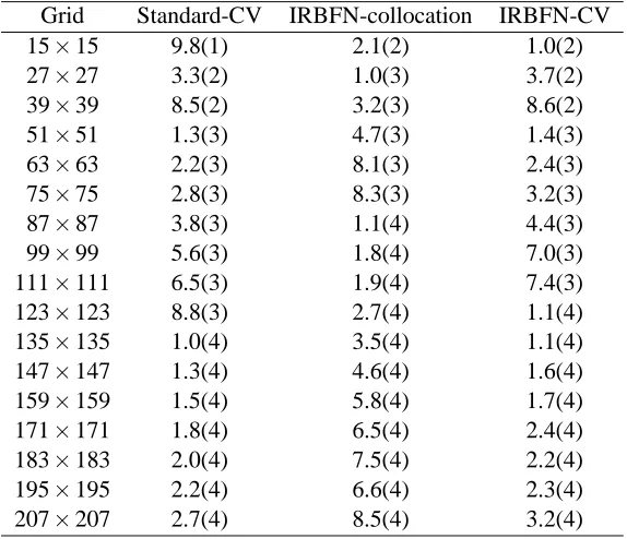
In the case of circular domain, the matrix condition number and the accuracy of the three methods are shown in Table 2 and Figure 4. Remarks for this case are similar to those for the rectangular case.

These numerical experiments indicate that the control volume formulation works better for local IRBFNs than the collocation formulation. The IRBFN-CV method is now applied to simulate some heat flow problem.

4.2 Heat flow

Find the temperatureθ such that

∇.

vθ₋ 1

Pe∇θ

=0, x_∈Ω, (27)

where v is a prescribed velocity, Ωthe domain and Pe the Peclet number. Here,Ωand v are taken as[0,1]_× [₋0.5,0.5]and(1,0)T_{, respectively. Boundary conditions are prescribed as follows}

θ=0, for x2=−0.5 and x2=0.5, (28)

θ=cos(πx2) for x1=0, and (29)

0 0.5 1 1.5 2

x 104 0

0.5

1

1.5

2 x 104

nz = 549081

Figure 3: Rectangular domain, 151_×151: The structure of the 22201_×22201 IRBFN system matrix.

10−3

10−2

10−1

100

10−7

10−6

10−5

10−4 10−3 10−2 10−1

Standard CVM

IRBFN Collocation

IRBFN CVM

h

N

e

(

u

)

Pe=10(21_×21)

Pe=100(51_×51)

Pe=1000(401_×401)

Table 2: Circular domain: Condition numbers of the system matrix by standard CV, local IRBFN collocation and local IRBFN CV methods. Notice that a(b)means a_×10b.

Grid Standard-CV IRBFN-collocation IRBFN-CV

15_×15 9.8(1) 2.1(2) 1.0(2)

27_×27 3.3(2) 1.0(3) 3.7(2)

39_×39 8.5(2) 3.2(3) 8.6(2)

51×51 1.3(3) 4.7(3) 1.4(3)

63_×63 2.2(3) 8.1(3) 2.4(3)

75_×75 2.8(3) 8.3(3) 3.2(3)

87×87 3.8(3) 1.1(4) 4.4(3)

99_×99 5.6(3) 1.8(4) 7.0(3)

111_×111 6.5(3) 1.9(4) 7.4(3)

123×123 8.8(3) 2.7(4) 1.1(4)

135_×135 1.0(4) 3.5(4) 1.1(4)

147_×147 1.3(4) 4.6(4) 1.6(4)

159_×159 1.5(4) 5.8(4) 1.7(4)

171_×171 1.8(4) 6.5(4) 2.4(4)

183_×183 2.0(4) 7.5(4) 2.2(4)

195_×195 2.2(4) 6.6(4) 2.3(4)

207_×207 2.7(4) 8.5(4) 3.2(4)

The exact solution to this problem can be verified to be

θe=

cos(πx2)

exp(a)₋exp(b)(exp(a+bx1)−exp(b+ax1)), (31)

where a=0.5

Pe+√Pe2₊₄π2_{and b=0.5Pe−}√_Pe2₊₄π2_.

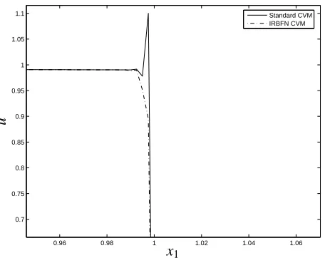
This problem is taken from [Kohno and Bathe (2006)]. The temperature boundary layer becomes thinner with increasing Pe. At Pe=1000, very steep boundary layer is formed. Figure 5 shows the temperature contours for three different values of Pe by the present CV method. Its accuracy is better than that of the standard CV method as shown in Table 3. Figure 6 displays variations of temperature along the centre line. It can be seen that the proposed method produces very accurate results for all cases. Figure 7 show that there are no fluctuations in the IRBFN CVM solution.

5 Concluding remarks

0 0.2 0.4 0.6 0.8 1 0

0.2 0.4 0.6 0.8 1

Pe=10

Pe=100

Pe=1000

Exact solution

x1

u

Figure 6: Heat flow: temperature values on the horizontal centreline for different values of Pe. Exact values are also included for comparison purposes.

0.96 0.98 1 1.02 1.04 1.06

0.7 0.75 0.8 0.85 0.9 0.95 1 1.05

1.1 Standard CVM

IRBFN CVM

x1

u

Figure 7: Heat flow: variations of temperature on the centreline in the boundary layer by the two techniques for

Table 3: Heat Flow, Pe=1000: Error Ne(u)by standard CV and local IRBFN CV methods. Notice that a(₋b)

means a_×10−b.

Grid Standard-CV IRBFN-CV

11_×11 2.69(-1) 1.00(-1)

51_×51 1.83(-2) 3.69(-3)

101_×101 4.25(-3) 9.36(-4)

151_×151 1.83(-3) 3.47(-4)

201_×201 1.01(-3) 1.75(-4)

251×251 6.45(-4) 1.11(-4)

301_×301 4.46(-4) 8.32(-5)

351_×351 3.27(-4) 6.92(-5)

401×401 2.50(-4) 6.15(-5)

standard volume techniques regarding accuracy for a given grid size, (iii) the local IRBFN control-volume technique is much more accurate than the local IRBFN collocation technique, (iv) the local IRBFN control-volume technique has the capability to produce accurate results for the simulation of flow problems having steep gradients.

Acknowledgement: This work is supported by the Australian Research Council.

References

Kohno, H.; Bathe, K. J. (2006): A flow-condition-based interpolation finite element procedure for triangular

grids. International Journal for Numerical Methods in Fluids, vol. 51, pp. 673–699.

Kosec, G.; Sarler, B. (2008): Solution of thermo-fluid problems by collocation with local pressure correction.

International Journal of Numerical Methods for Heat & Fluid Flow, vol. 18, pp. 868–882.

Lee, C. K.; Liu, X.; Fan, S. C. (2003): Local multiquadric approximation for solving boundary value problems. Computational Mechanics, vol. 30, pp. 396–409.

Mai-Duy, N.; Tanner, R. I. (2005): An effective high order interpolation scheme in BIEM for biharmonic boundary value problems. Engineering Analysis with Boundary Elements, vol. 29, pp. 210–223.

Mai-Duy, N.; Tran-Cong, T. (2005): An efficient indirect RBFN-based method for numerical solution of PDEs. Numerical Methods for Partial Differential Equations, vol. 21, pp. 770–790.

Patankar, S. V. (1980): Numerical Heat Transfer and Fluid Flow. McGraw-Hill.

Shu, C.; Ding, H.; Yeo, K. S. (2003): Local radial basis function-based differential quadrature method and its

application to solve two-dimensional incompressible Navier-Stokes equations. Computer Methods in Applied

Mechanics and Engineering, vol. 192, pp. 941–954.

Wright, G. B.; Fornberg, B. (2006): Scattered node compact finite difference-type formulas generated from