Applying the global standard FAO LCCS to map rural Queensland land cover

(1)

Applying the Global Standard FAO LCCS to Map Rural Queensland Land Cover

Kithsiri Perera, David Moore, Armando Apan, and Kevin McDougall

Keywords: FAO LCCS, Priori classification, Dichotomous Phase, Modular-Hierarchical Phase, Land cover classifiers. SPOT 10m data

Abstract:

With the introduction of satellite images, land cover map production developed rapidly. However it faced a common challenge to adopt an internationally accepted classification scheme. Most of the classification schemes were tailored to match local demands without flexibility to apply in other parts of the world. Land cover mapping in Australia is also facing the same dilemma, “the lack of standard classification system” to classify its massive land mass and compare internally and internationally. As a solution, in 2000, the Food and Agriculture Organization (FAO) produced a widely acceptable land cover classification system (FAO LCCS) which is based on priori (pre-decided) approach, to match with any region of the world. In this study we classified rural Queensland land cover, using the hierarchical and the priori method used by FAO LCCS. Under the priori approach, all classes are set before the classification, to maintain the standardization of categories. Then, a hierarchical dichotomous approach (divide into sub-categories) follows to achieve classes without having conflict between any two land cover types. We classified two rural Queensland regions, Hughenden grasslands and semi-arid Mt Isa. After classifying regions with level 1 to level 3 (FAO pre-set classes), classifiers based on spectral values and field investigations were implemented to build the level 4. Primarily, the classification used SPOT 10m data, other available information were utilized for the classification. Field investigation was carried out to verify uncertainties in spectral values and to collect ground information. Results of the study rendered well-classified two maps at 10m resolution for each area with over 80% overall accuracy. The most significant outcome of the study was the successful integration of FAO LCCS into local conditions of Queensland, which could serve as a guideline to map other regions in Queensland and other states of Australia.

1. Introduction

(2)

2

controlling primary productivity for terrestrial ecosystems can be defined in terms of land: the area of land available, land quality and the soil moisture characteristics (Di Gregorio and Jansen, 2000). This main resource or the Land further explains by its physical appearance as “Land Cover” and “Land Use”. The Australian institute under the Natural Heritage Trust, the National Land and Water Resources Audit, agrees with the FAO definition of the land cover, which is described as observed biophysical cover on the earth’s surface including vegetation and manmade surfaces (Di Gregorio, 2005). Further, the National Land and Water Resources Audit defines Land Use as the purpose to which the land cover is committed (National Land and Water Resources Audit, 2007).

[image:2.595.93.506.393.502.2]

This is explained further by the FAO definition; for example, “grassland” is a land cover type, while “rangeland” or “tennis court” refers to the “use” of respective “grassland”. Hence, it’s clear that the geographical feature of the land or land cover determines the land use. Also, ever increasing human interaction with the environment alters the land cover through dynamic changes in land use. Within last 50 years, the gross value of Australian agricultural sector expanded dramatically from $4.5 billion in 1960/61 to $46.5 billion in 2007/08 (Australian Bureau of Statistics, 2008). Due to its massive scale of activities, Australia has a significant obligation to act in this field of research to fulfill its local and global responsibilities in food production and environmental conservation. Table 01 shows few noteworthy features of Australian agriculture and land cover against world.

Table 01. Some characteristics of Australian agriculture and land cover (source: Agro data, 2006)

Component Australia World

Per Capita Cereal Production (tons per person), 1999 - 2001

1794 343

Percent change of Cereal production since, 1979-81 62% 32% Hectares of Cropland per 1,000 population, 1999 2547 251 Forest area as a percent of total land area, 2000 20% 29%

Land cover information is vital for the sustainable use of land. A standardized and up-to-date land cover dataset is required to; assess the condition of the natural resource base, modeling water quality, soil erosion, soil health and the sustainable production of food and fiber (DAFF, Australia, 2007). Data generation must be conducted to satisfy the logical approaches of standard land cover classification systems to compare with multi-temporal inter-state and international data. Here, the priori Land Cover Classification System (LCCS) adopted by the FAO can be used as the standard to build a local land cover classification system for Australia.

2. Constructing the classification scheme

(3)

3

Jansen, 2000). FAO and UNEP gathered in 1993 to establish a land cover classification system to match the wider spectrum of global land cover types and by 2000 the FAO LCCS became fully operational.

2.1 Basics considered in FAO LCCS

The FAO LCCS system is considered as the only such approach available today which can be applied to any region of the world regardless of the economic conditions and data source. Initially, the FAO method is a “priori” classification system, which defines all the classes before the classification is conducted. The advantage of this approach is the possibility to maintain standardisation of classes. For this proposes, LCCS developed pre-defined classification criteria, or classifier to identify each class, instead of identifying the class itself. This concept is based on the idea that a land cover class can be defined without considering its location or its type, using a set of pre-selected classifiers. Therefore, when the user requires a large number of classes, a large number of classifiers are required. To organize the classification more easily, FAO system used a dichotomous (divide into sub categories), approach in hierarchical levels and used eight classifiers to group all land cover types at the third level. In other words, any location on the earth surface can be categorized into one of the eight classes without having a conflict. Up to this third level, FAO used the presence of vegetation, edaphic (plant conditions generated by soil and not by climate), and artificiality of land cover for classification. Additionally, the third level of FAO classification can be considered as a concept based on visual classification, which uses the directly visible and knowledge based components on the ground.

[image:3.595.77.526.524.704.2]

In practical conditions, a further breakdown of the third level eight classes must be conducted to obtain a detailed level of land cover classes. For that purpose, FAO uses a hierarchical approach, or the Modular-Hierarchical Phase, to build additional classifiers, but strictly within one of eight classes identified in third level of the dichotomous phase. Under this 4th phase, the system uses a set of pre-defined pure land cover classifiers, different from the eight classes in the dichotomous phase presented in Table 02.

Table 02. Dichotomous approach to build primary classes in FAO LCCS First level Second level Third level

A. Primarily vegetated

A1. Terrestrial A11. Cultivated and managed terrestrial areas

A12. Natural and semi-natural terrestrial vegetation

A2. Aquatic or regularly flooded

A23. Cultivated aquatic or regularly flooded

A24. Natural and semi-natural aquatic or regularly flooded

B. Primarily

non-vegetated

B1. Terrestrial B15. Artificial Surfaces and Associated Areas

B16. Bare Areas

B2. Aquatic or regularly flooded

B27. Artificial water bodies, snow and ice

B28. Natural water bodies, snow and ice

(4)

4

(africover, 2003). In both cases, the user gets the freedom to add these classifiers with their own research interests, scale of the classification, and the physical and climatological conditions of the field. The FAO LCCS document presents a large number of classifiers to use in this level and the user can use only a selected set from the list to match with the scope of their own mapping project.

2.2 Australian vegetation and its recent changes

The Australian flora and fauna is a composite of Gondwanan elements, and has evolutionary lines shared with South America. About 80% of the flora of Australia is endemic to the country and most of the species are extremely restricted in geographic and climatic range. For example, 53% of the about 800 species of eucalypts have climatic ranges spanning less than 3˚C mean annual temperature, and 25% span less than 1˚C (Hughes, 2005). Also, about 23% have adapted to less than 20% of mean annual rainfall changes (Barrie, 2003). The recent global warming may have influenced these flora (and fauna), since the largely flat Australian geography offers only a little space to escape naturally.

(5)

[image:5.595.69.538.72.371.2]

5

Figure 1. Elevation and annual rainfall of Australia (source: Climate Data Online 2009)

2.3 Applicability of FAO LCCS system in Australian terrain

Australian land cover is greatly influence by climate rather than it’s near flat terrain with 99% of its land area below 1000m (Hughes 2005). Figure 1 compares the annual rainfall and topography of the country, which shows heavy rainfall along the east and north coastal areas. Within Queensland, the central region receives extremely low rainfall (Birdsville, mean annual rainfall is less than 200mm), while northeast coast receives heavy monsoon rains (Innisfail, mean annual is over 3200mm) (see locations on figure 1). Vegetation types throughout the state have adapted to these climatic variations. When classifying land cover of Australia, the priori classification approach of FAO LCCS, provides a logical approach to separate land cover types. It helps to ignore differences in land surface of Australia at the initial three levels of the classification (see Table 02). However, for the construction of the 4th level of the classification system, regional environmental features and field information must be considered.

(6)

6

3. The case study

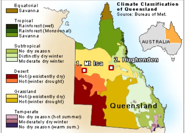
[image:6.595.146.449.236.453.2]

The land cover of Queensland varies from semi-desert barren lands and huge farm lands in the vast hinterland to some of Australia’s largest remnant tropical rainforests including a world heritage site (Department of the Environment, 2008) and urban environments in east coast. Mapping the land cover characteristics covering all these land cover diversities is a challenging task. The present study focuses on the classification of two selected locations of Queensland (see figure 2) that represent significantly different land cover types of the state. The paper presents two selected areas from originally classified full scenes of SPOT, with one area (area No. 1, Mt. Isa) in details.

Figure 2. Locations of study areas on QLD Climatic Zone map (data source: Climatemap 2010)

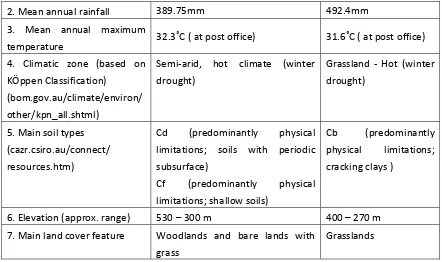
The locations of study sites are over 650 kilometres apart from each other (figure 2). The selected locations lie in the desert to grassland (Mt Isa) and grassland to subtropical (Hughenden) climatic zones respectively. The land cover classification of these two areas with contrasting geo-climatic characteristics makes the approach suitable to apply most of other Australian regions with appropriate modifications. As tabulated in Table 03, the two selected study areas are considerably distinct from each other by various geo-climatic aspects. The 1st area (around Mt Isa city in central Australia) has arid climate with relatively unproductive soil layer for farming (Michael and et al, 2005). Hughenden area (2nd study area) in central-northeast Queensland is in the massive Mitchell grasslands and closer to subtropical conditions of the state. For this study, we extracted 1000 km² sections from each region. Population density is very low and less than 2 people per 1 sq km (Australian Bureau of Statistics, 2008).

Table 03. Main features of study areas (sources: Climatemap 2010, Climate Data Online 2009, Soil groups 2006)

Element 1. Mt. Isa 2. Hughenden

(7)

7

2. Mean annual rainfall 389.75mm 492.4mm

3. Mean annual maximum

temperature 32.3˚C ( at post office) 31.6˚C ( at post office)

4. Climatic zone (based on KÖppen Classification)

(bom.gov.au/climate/environ/ other/kpn_all.shtml)

Semi-arid, hot climate (winter drought)

Grassland - Hot (winter drought)

5. Main soil types (cazr.csiro.au/connect/ resources.htm)

Cd (predominantly physical limitations; soils with periodic subsurface)

Cf (predominantly physical limitations; shallow soils)

Cb (predominantly physical limitations; cracking clays )

6. Elevation (approx. range) 530 – 300 m 400 – 270 m

7. Main land cover feature Woodlands and bare lands with grass

Grasslands

4. Data and data processing

4.1 Used data

[image:7.595.77.519.71.333.2]

Land cover maps were produced with SPOT 10m data, but number of other satellite images was utilized as supporting data. The Table 04 summarized the data sets used for the study.

Table 04. Used data in the study

Location / data type Data set identifier Date

Mt. Isa

SPOT 2.5m sthn_gulf_2p5m_nc.tif Not known

SPOT 10m sp5xi10_358391_30072005.tif

sp5xi10_358392_30072005.tif

30072005 30072005

ASTER 1397_203_130900.img 16102006

Landsat l5tmre_mtis_20051005_ba7m4.img 05102005

Field Survey Dec/Jan 2008

Hughenden

SPOT 10m sp5xi10_367390_16072005.tif

sp5xi10_367391_16072005.tif

16072005 16072005

ASTER 1437_205_240900.img 16102006

Landsat l5tmre_hugh_20050728_ba7m4.img

l5tmre_oakv_20050813_ba7m5.img

28072005 13082005

(8)

8 4.2 Building the classification for study areas

The methodology of building the classification scheme focuses on one of the mapped areas, Mt Isa in north-west Queensland, in order to limit the length of the paper. For all the aspects of image processing, Micro Image TNT software package (TNTmips 2008:74) was used. The construction of first three levels of the classification was completed by strictly following the FAO LCCS structure. For these initial three levels, spectral characteristics of SPOT images and vegetation index image were used extensively. Different levels of spectral information were also used to isolate broad classes at each level of the LCCS. A new set of training sites was selected from each level to perform the next level classification. Those training sites were selected with the help of 2.5m SPOT images, field investigations, different image indexes of SPOT, Landsat, and ASTER data, and general knowledge of the region. Under the dichotomous approach (see table 2) of FAO LCCS, the accuracy of each initial level permanently is affected to the accuracy of following levels of the classification.

4.2.1 Classification Level I: A supervised classification to isolate non-vegetated lands was

conducted through careful selection of training sites from 100% non-vegetated areas. Spectral values of each SPOT band and NDVI image together with 2.5m SPOT images were used to identify these training sites, precisely. All other areas under different levels of vegetation (from vegetated area to a mix of bare ground and grass) were classified into vegetated areas.

4.2.2 Classification Level II: The re-classification was carried out with two classes of level I to generate four classes. After observing the NDVI, image classification was conducted through selecting training sites using the 2.5m and 10m SPOT images. Only 3 classes were found out of four, and the class A2 (“aquatic or regularly flooded areas under primarily vegetated category”) (see figure 3) were not found in Mt Isa region.

4.2.3 Classification Level III:In the 3rd level, FAO LCCS has 8 sub classes to represent all land

surface features on the earth. The availability of the area under each class is directly depending on the regional features of land cover of each respective area. A clear example is, in a remote desert region with no human settlements or any vegetation, it may just comprise of only one class (B16, A6: Loose and Shifting Sand) from these 8 classes. The Mt Isa region has a predominantly dry climate and no vegetated lands under aquatic or regularly flooded conditions exit. We found five classes out of eight original classes at this level (see Level III in figure 3) with regard to Mt Isa region.

4.2.4 Classification Level IV:The 4th level of the classification is the challenging phase of the

(9)

9

[image:9.595.85.513.188.660.2]

In this study we used very high resolution 2.5m satellite images and ground survey information to build classifiers for the 4th level. Additionally, spectral characteristics of SPOT 10m images played a strong role in the classification process. Figure 3 shows the simplified flow of this process, which presents all four levels with regard to the Mt. Isa map. Classifiers used under FAO system to generate each class in level IV for Mt Isa map are presented in Table 05.

Figure 3. Building the classification scheme according to the FAO LCCS.

(10)

10

Class Code

Class name Classifiers FAO LCCS Classifier Codes

A11.3. Cropland Visually identified training sites using 2.5m data and field investigation + high NDVI value (around 0.6)

A11

A3 Herbaceous D4 Surface irrigated

A12.1. Woody vegetation

Visually identified training sites using 2.5m data and field investigation + high NDVI value (higher than 0.3) + closed woodlands (> 60%) + tree height is over 2.5m

A12

A1 Woody A1 A10 Closed A10 B1 Height 7 – 2 m

A12.2. Low Woody vegetation

Visually identified training sites using 2.5m data and field investigation + high NDVI value (higher than 0.3) + open woodlands (10 – 40%+ tree height is over 1m

A12

A1 Woody A21 Open

B14 Height 5 – 05m

A12.3. Savannah Visually identified training sites by smooth texture on 2.5m image + areas under low NDVI value (below or around 0.3), and Shrubs (Sparse) + Graminoids observed from field investigation

A12

A4 Shrub A6 Graminoids

A14 Sparse (1% - 15% Shrubs and trees)

A12.4. Grassland (wetlands)

Visually identified training sites by smooth texture on 2.5m image + areas with moderate to high NDVI value (0.3 - 05), dominate by Graminoids observed from field investigation

A12

A6 Graminoids C1 Spatial distribution

A12.5. Grassland sparse

Visually identified training sites from areas under low NDVI value (below 0.3), with Sparsely distributed Graminoids, observed from field investigation

A12

A6 Graminoids A14 Sparse

A12.6. Grassland/tr ee/ sparse

Special spectral feature of soil color caused by rocky terrain, identified by 10m and 2.5m data, verified by field investigations.

A12, A6 Graminoids A4 Shrubs, A14 Sparse A3 Tree Sparse A14

B15.1. Built-up Visually identified training sites using 2.5m data and field investigation

B15

Urban Areas A13

B15.2. Built-up/soil Visually identified training sites using 2.5m data and field investigation

B15

A12 Industrial and other

B16.1. Bare soil Visually identified training sites using 2.5m data and field investigation

B16

A5 Unconsolidated Bare soil

B28.1. Inland water Visually identified training sites using 2.5m data B28. A1 Water

(11)

11

This paper mainly emphasizes the characteristics of Australian land surface and the application of FAO LCCS to classify that into land cover classes. We produced land cover maps for the two test sites mentioned in previous sections.

5.1 Mt. Isa, the arid region

The vicinity of Mt Isa city significantly represents the vast inner Australian arid landscape. The centre of the mapped area (Mt Isa city) associates with a large mining complex, which is one of the largest in Australia. The built-up area of the city with 23,000 people is restricted to a small area, though its urban limits cover 43,310 square kilometres (Mt Isa city council, 2008). Due to the harsh climate, no major farming areas can be seen closer to the city, except ranching activities. Figure 4, shows typical red-soil outback (Australian term for remote area) environment around Mt Isa.

Figure 4. Typical land cover types in Hughenden (top 2 photos) and Mt Isa area.

Through a careful observation of spectral characteristics of SPOT 10m images and vegetation index images as explained in section 3.3, a land cover map of Mt Isa was produced with 11 classes under the 4th level (figure 5). An accuracy assessment of the Mt Isa map was carried out using the 2.5m SPOT image. Using a systematic random sample, 128 points were selected from the area covered by 2.5m image and checked against the classified image data. Samples were under represented on land cover types with very low areas of coverage, but all major land cover types were counted. Results showed an overall accuracy of 82% for Mt Isa map.

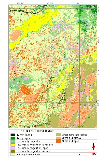
5.2 Hughenden, the grassland region

(12)

12

identified as the dominant land cover type in Hughenden area (figure 6). Large cattle farms are spread all over the area with extremely low number of permanent settlements. Image processing methods used for Hughenden image were same as methods used for Mt Isa map. Also, spectral characteristics clearly helped to separates some classes within woody vegetation, where soil types have influenced to for tree types on respective soil type (Class A 12.6, Low woody vegetation on slopes). The figure 7, shows an area for these vegetation type changes along the rocky slopes and fertile table-shape mountains and valleys with grasslands and riparian forests. We noticed some deviation of spectral signatures on images with the ground survey evidences, mainly due to wet weather followed after the image date in Hughenden.

(13)

[image:13.595.133.479.67.574.2]

13

Figure 5. Land cover map of Mt Isa region.

5.3 The qualitative aspects of new maps

(14)

[image:14.595.126.472.67.571.2]

14

Figure 6. Land cover map of Hughenden.

We have used an approach based on spectral values and visual observation of super-resolution (2.5m colour images), which are the basic needs for any classification. We then added field observation information to the training site selection and the refining process, which strengthens the classifiers used to break level 3 classes into the 4th or final level classes. As explained earlier, the classification gave satisfactory levels of accuracy with both maps being accommodated in a classification scheme based on FAO system.

(15)

15

Class Code

(Arranged by FAO LCCS)

Class Name in Hughenden map Class Code

(Arranged by FAO LCCS)

Class Name in Hughenden map

A11.1. - A12.9. Grassland closed

A11.2. - A12.10. Grassland open

A11.3. Cropland B15.1 -

A11.4. - B15.2 -

A11.5. - B15.3 -

A12.1. Woody closed B15.4 -

A12.2. Woody open B15.5 -

A12.3. Low woody vegetation B16.1 -

A12.4. Low woody vegetation in red soil B16.2 -

A12.5. Low woody vegetation, open B27.1 -

A12.6. Low woody vegetation on slopes B28.1 Inland water

A12.7. Mix vegetation closed B28.2 -

[image:15.595.68.530.78.536.2]

A12.8. Grass/herb land closed

Figure 7. A selected location of Hughenden map shows its relation to the actual land cover types on the ground. (1) Low woody vegetation on slopes (2) Low woody vegetation, open

(3) (Riparian forest) Woody closed, Woody open, Low woody vegetation (4) Grassland closed

.

(16)

16 photo taken date.

6. Conclusions

Australia’s agriculture and mining based economy requires an accurate assessment of land use and land cover. However, mapping the country at 10m or finer resolution has just started and over 90% of the country is yet to be mapped. This study classified two distinctly different landscape plots in Queensland, Australia. The prime objective of the study was to build the classification system common for both regions using the fundamental approach of FAO Land Cover Classification System (FAO LCCS). The FAO LCCS has three initial class levels based on a priori (pre-defined) classification approach and the 4th detail level or the Modular-Hierarchical Phase. A careful observation of the spectral information against super resolution satellite data and ground survey information enabled classifiers for 4th level to be selected. For each map, different land cover types were identified in diverse geo-physical and climatic conditions for each respective region. Some classes ended with same name and same class identifier when the classifiers were similar to each other (e.g.; A12.2. woody open class in Hughenden map). The results showed a promising outcome for mapping different rural regions of Australia under a single classification scheme introduced by FAO. The maps were completed with a high accuracy and 10m spatial resolution will be a useful planning tool as well as a guide for mapping rest of the state as well as other rural areas of the country.

Acknowledgements:

Authors are thankful to Mr. Jeremy Hayden of Southern Gulf catchments for providing satellite data and facilitating field investigation opportunity in Mt. Isa region.

References:

Africover LCCS, FAO: 2003, online document, http://www.africover.org/LCCS_hierarchical.htm

Agro data; World Resource Institute, 2006 http://earthtrends.wri.org/text/agriculture-food/country-profile-9.html

Atyeo C. and Thackway R., 2006, Classifying Australian Land Cover, Australian Government, Bureau of Rural Sciences

Australian Bureau of Statistics, 2008, http://www.ausstats.abs.gov.au/ausstats/

Barrie Pittock, 2003, Climate Change: An Australian Guide to the Science and Potential Impact. Australian Government agency on greenhouse matters, 94-101 pp

Butt P, 2001: Land Law, Law Book Co of Australasia, 2001 http://www.teamlaw.org/LandDef.htm

Climate Data Online 2009, http://www.bom.gov.au/climate/averages/

(17)

17

Department of the Environment, Water, Heritage and the Art, 2008, Gondwana Rainforests

of Australia,

http://www.environment.gov.au/heritage/places/world/gondwana/information.html

DAFF (Department of Agriculture, Fisheries, and Forestry), Australia, 2007, http://www.daff.gov.au/

Di Gregorio A., FAO Land Cover Classification System, Classification concepts and user manual, software version 02. 2005

Di Gregorio A.., and Jansen L. J. M., 2000: Lands cover classification system (LCCS), FAO.

Hughes L., 2003, Climate change and Australia: trends, projections and impacts. Austral Ecology 28, 423-443.

Hughes, L., 2005: Impacts of climate change on species and ecosystems: an Australian perspective, The International Biogeography Soc., Summer 2005 Newslet.: Vol. 3, No. 2

Michael F.H., Sue M., Richard J. Hobbs, Janet L. Stein, Stephen G. and Janine K.: 2005, Integrating a global agro-climatic classification with bioregional boundaries in Australia. Global Ecology and Biogeography, 14, 197-212

Mt Isa city council, 2008, http://www.mountisa.qld.gov.au/

National Land & Water Resources Audit, 2007, Australian land cover mapping, http://www.nlwra.gov.au/

Soil groups, 2006, Resource material on desert Australia http://www.cazr.csiro.au/connect/resources.htm

State of the Environment, 2006: Independent Report to the Commonwealth Minister for the Environment and Heritage. Australian State of the Environment Committee. Land and Vegetation section, www.environment.gov.au/soe/2006

There are four (04) authors in this paper and Kithsiri Perera is the corresponding author.

Contact Information Name Kithsiri Perera(corresponding author)

Company/Institution Faculty of Engineering and Surveying and Australian Centre for Sustainable Catchments

Address University of Southern Queensland, West Street, Toowoomba 4350 QLD Australia

(18)

18

Email perera@usq.edu.au

Contact Information

Name David Moore

Company/Institution Terranean Mapping

Address Terranean Mapping, PO Box.729, Fortitude Valley, 4006 QLD Australia

Phone number Fax number Mobile number