Understanding school financial decisions

(1)

Research Report DFE-RR183

Understanding school

financial decisions

Rebecca Allen, Institute of Education, University of London

Simon Burgess, Centre for Market and Public Organisation, University of Bristol

Imran Rasul, University College London

Leigh McKenna, Centre for Market and Public Organisation, University of Bristol

(2)

This research report was commissioned before the new UK Government took office on 11 May 2010. As a result the content may not reflect current Government policy and may make reference to the Department for Children, Schools and Families (DCSF) which has now been replaced by the Department

(3)

Executive

Summary

With over £30bn of public money spent every year, English schools face complex financial decisions that relate almost exclusively to their spending. In this Report, we analyse the degree of variation in expenditure items between schools, and examine how much of that variation is due to their circumstances, and how much reflects specific decisions made by the school. Lastly, we consider the potential for improvements in resource utilisation. Although these issues have been addressed before, most of the existing literature focuses on overall school expenditure. Thus we contribute in a number of ways:

1. By exploiting a new dataset, we can examine schools at a very disaggregated level and isolate some of the real operational decisions that they make on how to allocate their budgets. The new School Workforce Census covers all employees in all schools in the country, and includes

information such as age, pay and tenure;

2. We control in considerable detail for the schools’ circumstances to ensure that we are focusing on schools that are facing the same operational environment;

3. To better understand discretion over expenditure, we analyse what schools do with their “residual” income. That is, income which is not accounted for by their circumstances;

4. We use data over two years to examine how schools adjust their spending in response to changes in their income.

Results

–

Commentary

(5)

Another important set of restrictions comes from the institutional setting around teacher pay and conditions, negotiated between trade unions and government. While some of these restrictions have been relaxed in recent years for some schools, there has been little change to date in practice. But perhaps more important than the constraints is the lack of incentive for school leaders to get spending decisions right. A careful and considered allocation of spending that approximates an optimal allocation makes little difference to a headteacher and her/his leadership team, who tend to be focused on overall pupil achievement – an outcome that we know reflects little on input decisions. Severe financial mismanagement is obviously a serious issue, but spending (say) three times as much as comparator schools on support staff is not. The simplest answer to the question “How can we improve schools’ financial decisions?” is “Make them matter”. By using insights from economics, psychology and behavioural economics, we attempt to shed light on this question

Results

–

Summary

(6)

58% of schools choose to increase the majority of their expenditure on other items, or allow their budget balance to change the most.

Introduction

Each year schools in England spend over £30bn of public money. Put another way, the state spends over £50k per pupil over her or his time in school, and this expenditure is managed by schools. Schools are much more than simply a team of teachers in classrooms, with the typical secondary school employing over 100 people of whom only around half might be regular classroom teachers. In the private sector an organisation with 100 employees would count as a medium‐sized firm, and just like such a firm, schools have complex managerial decisions to make. The financial decisions that schools have to take are almost exclusively about their spending. To a large degree, schools simply receive income on the basis of the number and characteristics of their pupils (though to a small and decreasing extent they can also seek and receive specific grants to do specific things). Schools, by and large, then spend what they’re given although as shown later in this report, some schools choose to build their balances rather than increase exenditures, in response to increases in their income. So an analysis of schools’ financial decisions is essentially about how budgets are allocated between different items within a particular year. It should be obvious that it matters how money is spent on additional resources. The Department’s

Improving Efficiency in Schools notes: “What matters isn’t the amount of money spent per pupil, but

how that money is spent” (para 11). Schools have a great deal of discretion over expenditure on capital and labour inputs, but are they spending the money effectively? There is a large literature on overall school expenditure and school outcomes, and on certain individual spending items such as number of teachers per pupil, but much less on analysing the details of school expenditure patterns and the extent of schools’ discretion over expenditure. This report is concerned with the variation in expenditure between schools and the potential for improvements in resource utilisation. It exploits a new data source to analyse at a very disaggregated level, how schools’ allocate their financial budgets between different inputs. We are able to use this new data source to ask: How much variation is there in expenditure patterns for schools which appear to be in very similar operational circumstances? Do their actions reveal an implicit agreement on best practice? Or is diversity of response the key message? We analyse the degree of variation in expenditure items between schools. This has been addressed before for some headline spending totals, for example in the Department’s publication Improving

Efficiency in Schools (DfE, undated), and by the Audit Commission (2011). We add to this evidence in

a number of ways:

(7)

of the School Workforce Census, covering all employees in all schools in the country. This means we can, for example, consider the following factors:

• Expenditure on classroom teachers and on senior managers per pupil;

• Proportion of support staff on short‐term contracts;

• Proportion of teaching staff with tenure less than one year;

• Age and pay of the Headteacher;

• Proportion of teachers with qualification in their main teaching subject;

• Proportion of hours of maths taught by qualified subject teachers;

• Estimated school‐level pay premium.

2. We control in considerable detail for the schools’ circumstances so that we are confident we are focusing on schools that are facing the same operational environment;

3. We analyse what schools do with their “residual” income, explained below;

4. We look at how schools adjust their spending in response to changes in their income over time.

Can we use evidence on differences in expenditure to improve school efficiency? This is difficult because the evidence (briefly reviewed below) shows that there is at best a small and statistically weak relationship between schools’ expenditure and their outcomes, the level of pupil attainment. This is a problem and a puzzle.

It is a problem because the allocation of larger government budgets is the usual means by which governments attempt to improve the public services they value most. For example, the first decade of the Labour government in the UK produced a 56 percent real increase in school budgets with very large rises for the most deprived schools; yet, the empirical evidence suggests that this attempt to improve schools and to close the social class gap in attainment may not reach its policy goals. Indeed, the increased expenditure has not seen outputs rise at the same rate, and so school productivity has fallen (Wild et al., 2009).

It is also a puzzle. Why does increased spending not necessarily raise outputs by much? It tends to in other contexts. By definition, schools must be spending the money ineffectively. Are they spending money on the wrong things? If so, why? Before this publication of the School Workforce Census it was not possible to analyse workforce composition properly, which is critical in organisations where staff spending accounts for almost 80% of current expenditure. This is why we believe this type of analysis is critical to understanding opportunities to influence the behaviour of school managers. This report contributes to the answer to this puzzle by analysing in great detail the things that schools buy, and considering the possible reasons behind the patterns that emerge.

(8)

(9)

The simplest answer to the question “How can we improve schools’ financial decisions?” is “Make them matter”. We provide a more detailed commentary on this in the Conclusion, bringing in insights from economics, psychology and behavioural economics.

Review

of

the

Evidence

The

overall

relationship

between

school

income

and

quality

(10)

and concludes that reducing the teacher pupil ratio was an effective way to improve standards. The implications of Krueger’s study are that resources can improve educational standards if utilised effectively. For the remainder of this section, we focus on individual items of school expenditure. As will be evidence, for some types of input there are large literatures, and a much weaker evidence base for the effectiveness of expenditures on other types of input.

Class

size,

the

quantity

and

deployment

of

teachers

The impact of pupil‐teacher ratios on student performance has been extensively studied in many countries. Some studies have been able to use experimental data such as in the Tennessee STAR experiment. In the project, the performance of students in larger classes (24‐25 students) was compared to that of students in smaller classes (15‐17 students). Whilst there is still some controversy over the class size findings in the STAR experiment, one of the authors of the original study (Kreuger and Whitmore, 2001) argues that “Overall, Project STAR indicates that reducing class size is a reasonable economic investment: the benefits are sizeable and long‐lasting, especially for black students, and the overall benefits outweigh the costs.” (Schanzenbach, 2006). It is important to note that the experiment and the evidence relate only to young pupils, in junior elementary school. Some interesting new research however, suggests that the real lesson of project STAR might lie in teacher and peer group quality rather than class size (Chetty et al, 2010). Turning specifically to UK evidence, a set of studies use the National Child Development Study (NCDS), a cohort of individuals born in 1958, to estimate the impact of class sizes on attainment and staying‐on rates. The estimated impacts are all either zero (e.g. Feinstein and Symons, 1999; Dearden et al, 2002) or relatively small. For example, Dustmann, Rajah and van Soest, 2003, find a one standard deviation increase in average class size decreases the probability that pupils stay on in education by about 4 percentage points; Dearden et al., 2002, find some wage impact for women only. There is a little evidence on the impact of learning support and individualised learning. Machin et al. (2007a) use a difference‐in‐difference framework to analyse the effects of the Excellence in Cities (EiC) programme in the UK on Key Stage 3 outcomes. The programme allocated additional resources to disadvantaged schools within participating Local Education Authorities (LEAs), with schools required to spend the money on one or more of three core areas: learning mentors to overcome educational or behaviour problems; Learning Support Units to provide short‐term teaching and support for difficult students; a Gifted and Talented programme, to provide extra support for 5‐10 per cent of pupils in each school. The authors find that over time the programme had a positive effect on school attendance as well performance in mathematics, although not in English.

Teacher

quality

(11)

one area where more research is clearly needed, but we do know that teachers, like all workers, are attracted to higher wage opportunities, with studies confirming that salaries and working conditions affect the probability of applying for a job and leaving a school (e.g., Dolton and Van der Klaauw 1999). Economists are now starting to quantify classroom practices and correlate these with measures of student attainment and teacher effectiveness (see Kane et al (2010) and Lavy, 2011).

Teaching

Assistants

The number of Teaching Assistants (TAs) trebled from around 60,000 in 1997 over the next decade. A substantial fraction of the additional resources available to schools was spent on TAs, in part in response to the Workload Agreement aimed at removing some duties from teachers. While to our knowledge there have been no randomised control trials evaluating their role, a series of studies that have been carried by Blatchford and others have concluded that the presence of TAs has little direct impact on the grades achieved by their pupils (Blatchford et al (2007). There may be indirect effects on the effectiveness of teachers, for example “more individualised teacher attention” but it is unclear whether this has any measurable impact on attainment.

Resources

(12)

Data

Our analysis combines four datasets, Edubase, the National Pupil Database (NPD), the Consistent Financial Reporting (CFR) accounts database and the first full collection of the School Workforce Census (SWC). The data is linked using the school establishment number which is common across all datasets. Our criteria for inclusion is simply that the school must have either an SWC record in November 2010 or a CFR record for 2009/10. Many schools we include do not have both: notably academies are not required to submit CFR accounts and newly opened schools in September 2010 will not yet have CFR. We categorise all schools as either primary or secondary using the DfE‐ standard approach for non‐standard entry schools. All special schools are excluded from the analysis.

National

Pupil

Database

and

Edubase

Edubase contains an administrative record for all schools, whether maintained or private, in

England. We use this to construct information on the structural characteristics of each school so that we are able to compare schools to similar schools in our analysis. The distribution of the structural factors we use from Edubase are summarised in Data Appendix Table 1 and include:

• government region indicators (with additional indicators for the Inner, Outer and Fringe London pay regions since these are important unavoidable factors that determine costs for a school);

• four indicators for whether school is rural, in a village, town or dense urban area;

• school age span (highest and lowest ages of pupils);

• school governance type and whether it is a single‐sex, grammar or boarding school;

• the number of full‐time equivalent pupils (also squared, cubed and to power four) and also the official school capacity; and

• nursery school presence indicator and size, sixth form indicator and size.

We use the NPD, a DfE administrative database of all pupils in state‐maintained schools in England, to measure the demographic background of the school. The NPD contains a wide range of

information on pupil characteristics including test score histories, ethnicity and age. Pupil characteristics and test histories are aggregated at the school level to allow us to group similar schools together. The distribution of the demographic factors we use from the NPD are summarised in Data Appendix Table 2 and include:

• fractions of pupils with English as an additional language;

• the fraction and type of special educational needs of pupils at the school;

• the proportion female (also squared) and ethnic composition of the school;

• the fraction of pupils eligible for free school meals (also squared);

• measures of the average neighbourhood deprivation of the schools’ pupils (also squared);

(13)

Consistent

Financial

Reporting

2009

‐

10

DfE has publicly released the CFR accounts for 2009/10 in full for the first time. The data contains information on income and expenditure in all state‐maintained primary and secondary schools in England with the exception of Academies. The income and expenditure data are split into 17 and 32 categories respectively; all expenditure or income of a school is included in exactly one category. Due to the limited number of streams of income schools receive, the income categories are generally specific (e.g. income delegated by the LA, SEN Funding, and so on), whereas the expenditure categories often comprise of many similar items grouped together (e.g. teaching assistants, learning mentors and behavioural managers staff costs are all grouped into the education support staff category). Some items in the CFR are censored when there are small numbers of employees in a role in a school or when schools spend (or receive) less than some threshold in a staff related category. As a result of this there is a missing data problem for some primary schools but secondary schools remain largely unaffected. Due to the limitations of the data, when we wish to conduct analysis on specific roles (e.g. expenditure on teaching assistants or senior management staff) we must refer to the SWC dataset, described below. We use CFR data in two ways in our analysis. Firstly, we often want to compare schools with similar incomes and where we do this we use the total income from all sources per pupil, with powers of two, three and four included where relevant. Secondly, we create a series of financial characteristics of the school that are summarised in Data Appendix Table 3 and include: • Total income per pupil; • Total expenditure per pupil; • Teaching expenditure per pupil;Expenditure on education support per pupil.

School

Workforce

Census

(14)

There are two major data quality problems with SWC: some variables are missing, and for other variables included, there are apparently missing observations. The missingness on variables is a particular problem for indicators such as teachers’ qualification (65% missing) and subjects taught in the classroom (68% missing). Although the SWC includes information on all staff, detailed pay information was only made available for teachers (including head teachers) and teaching assistants. As a result of this pay information is missing for around 90% of support staff and 10% of teaching assistants. The very large variation in staff‐pupil ratios across schools lead us to suspect that some schools have failed to submit a return for every member of staff and this should be borne in mind during the analysis section. This may also be an aspect for future waves of SWC to tighten up on.

We use SWC to create a series of financial and operating characteristics of the school that are summarised in Data Appendix Table 3 and include:

• Expenditure on classroom teachers per pupil, defined as the sum of gross pay, adjusted by full‐ time equivalent indicators, for classroom teachers who are not assistant, deputy or head teachers;

• Expenditure on senior management per pupil defined as the sum of gross pay, adjusted by full‐ time equivalent indicators, for assistant, deputy and head teachers;

• Number (FTE) of senior managers in school;

• Proportion of teaching staff under age 30;

• Proportion of teaching staff with qualified teacher status (QTS);

• Proportion of support staff on short‐term contracts;

• Proportion of teaching staff with tenure less than one year;

• Age of the Headteacher;

• Pay of the Headteacher;

• Proportion of teachers with qualification in their main teaching subject;

• Proportion of hours of maths taught by qualified subject teachers;

• Proportion of hours of English taught by qualified subject teachers;

(15)

(16)

Detailed

Results

We first characterise the differences in schools’ decisions on their spending patterns. We supplement that with an analysis of how the ‘residual’ income schools receive is spent, and an analysis of how a change in income is allocated across spending items.

Part

1:

How

much

variation

in

spending

is

there

for

‘like’

schools?

(17)

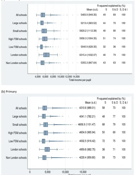
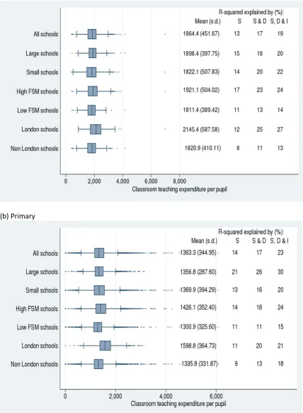
The box plot is a standard tool for giving a sense of the degree of variation. It displays the median, and the upper and lower quartiles of the distribution, thus showing both variation (the inter‐quartile range, IQR) and location (where the middle half of the data lie). In addition the box plot also indicates the location of points further out from the bulk of the data. The lines extending from the box finish at the upper and lower adjacent values. The upper adjacent value is the largest observation that is less than or equal to the third quartile plus 1.5*IQR. The lower adjacent value is the smallest observation that is greater than or equal to the first quartile minus 1.5*IQR. Outliers are all values that fall outside either of these points, and the plot shows some outlier values too to illustrate very extreme outcomes. Next to each box‐plot we summarise how much variation in the variable of interest is explained by schools’ structural factors, the demographic profile of the schools, and the schools actual income. We want to do this to assess how much variation is due to the schools’ circumstances and how much is the result of discretion, decisions that schools have taken on how to deploy their resources. To do this, we present the R2 statistic from a series of regressions, for each variable of interest, for each group and for primary and secondary schools. The R2 statistic measures what percentage of the variation in the dependent variable is accounted for – explained by – the explanatory variable. A high value, close to 100%, shows that there is little discretion and most of the differences between schools in their spending in this particular category are simply driven by their observable

characteristics. A value of the R2 near zero suggests that differences in expenditure are essentially idiosyncratic – that schools in the same circumstances are spending very different amounts. These R2 statistics are therefore key in answering the question we are addressing here. We use R2 rather than

(Rbar2) because we are interested in the total cumulated explanatory power of all the variables at our disposal. For each expenditure variable and each school group we run three regressions. The first is conditional on what we call structural (S) factors, the second regression adds demographic (S & D) factors, and the third adds the schools income (S, D & I). As described in the data section, the structural factors are created from Edubase and include size and type of school. The demographic factors are created from NPD and include the average prior attainment and average social characteristics of the pupils. The school income from CFR is total income from all sources per pupil, with powers of two, three and four included. The idea is that we want to isolate and remove variation conditional on unavoidable structural characteristics that impose costs on the school. Second, we want to also take out variation

conditional on demographic characteristics that schools need resources to help deal with1. Finally, we want to condition on the income that schools actually receive, giving them the opportunity to spend money. There are a number of preliminary points to make about these regressions that apply to all the charts below. First, we expect that in general the final regression, which adds actual income on top of structural and demographic factors, will not add a great deal of explanatory power. This may

(18)

seem counter‐intuitive since income constrains expenditure, but the school’s income depends quite heavily on these structural and demographic factors, and therefore implicitly the second regression is controlling for ‘expected’ income. So the interpretation of the final R2 is how much more of the variation in expenditure can we explain if we know the schools ‘residual’ income as well. Because of the importance of this issue, we undertake a more explicit analysis of this in part 2 of the Results.

Second, adding further explanatory variables has to always increase explanatory power. In terms of the regressions then, the value of the R2 should always increase from the first (S) to the third (S, D & I) regression. In practice this does not always happen as the sample varies, particularly when we add income (which is missing for new schools and academies). We chose to allow this to happen and to maintain the maximum sample per regression rather than use a restricted sample across all specifications. Results We present our analysis of variation in expenditure, demonstrating different approaches to measuring particular expenditure items. Our first results are for overall expenditure, and then show results for teaching staff, senior management teams and support staff.

Variation in total income and expenditure

Income is clearly not an expenditure item but we include it here to benchmark the overall amount of variation in the resources available to schools. Following the approach in the methodology, Figure 1 combines the box plots of total income and the R2 results of 3 regressions per group.

(19)

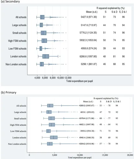
rationale for both MFG and ‘spend‐plus’ in terms of financial stability and planning convenience, the negative aspects of these policies need to be acknowledged too. Unsurprisingly given the similarity between total income and total expenditure, the pattern of results for total expenditure in Figure 2 are very similar. There are some extreme outliers of very high expenditure per pupil, particularly for primary schools. Almost all the variation is explained once income is included, the difference being driven by schools’ decisions to allow the balance between income and expenditure to adjust (see also section 3 below).

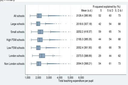
Variation in teacher expenditure

(20)

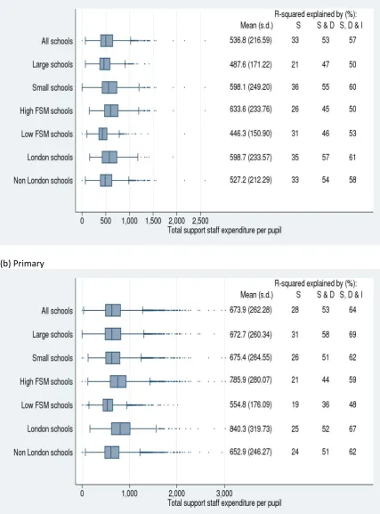
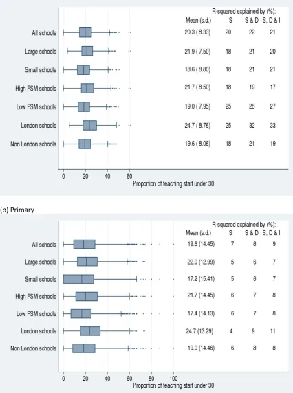
(Note that in the regression sample, the overall mean effect is zero, but is not here as schools have had to be dropped from this analysis sample.) Figure 18 shows that there is little difference in the average pay premium other than for London schools, but some variation within groups. The overall standard deviation of £2.5k is small relative to mean teacher pay of around £40k. This is perhaps not surprising given the very high use of the standard teacher pay scales. About half of this variation is explained by structural and demographic factors and by income, so there is evidence of some use of discretion in this. There are a number of measures for the likely levels of qualifications and experience of the teacher workforce. Firstly, Figure 9 shows the proportion of teachers with qualified teacher status (QTS). There is very little variation in this across schools. The averages are all in the high 90s, and there are only outliers below 90%. This is slightly less true in London, and in deprived schools. Figure 8 shows the proportion of teaching staff under age 30 and Figure 11 shows the proportion of teachers with tenure less than a year. Both these might act as good proxies for teachers’ overall experience in the absence of a SWC variable that measures total number of years in teaching. In Figure 8 there are small differences between group averages and relatively less variation. There is more variation – and mostly unexplained – among primaries. These schools are smaller so more susceptible to random variation in teacher age. Figure 10 shows the proportion of non‐teaching staff on short‐term contracts, but again we have concerns about the data quality here in the SWC as much of this information is not reported. The mean is 91% in all the groups in secondary schools and a little bit lower in primaries. Overall, there is little variation. The short‐tenure variable shown in Figure 11 includes senior management team teachers. Quite different to what might have been expected given received wisdom, we find very little variation in the averages between the groups of schools. For example, there are only slightly more short‐tenure teachers in high poverty schools than low. This is a finding that we confirm in our more extended investigation of tenure distributions. There is also quite a lot of variation within groups and variation is marginally greater among small schools and poor schools. The variation is not explained by the structural factors, nor explained by demographics, nor income (again, note that the sample varies considerably in the final column explaining the ‘fall’ in the R2).

(21)

relative importance of core subjects against more specialist subjects (such as photography, or citizenship). Figures 15, 16 and 17 show the proportion of pupil hours taught by specialist teachers in maths, English and science, respectively. Again there is a smaller sample of schools here. The levels are lower in small schools, typically they will need more flexible teachers and fewer specialists. Figure 17 shows that there are slightly more specialists in science. There is considerable variation within all the groups with the inter‐quartile range covering much of the entire range of data. No more than a quarter of the variation is explained.

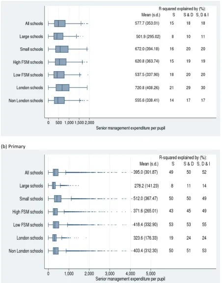
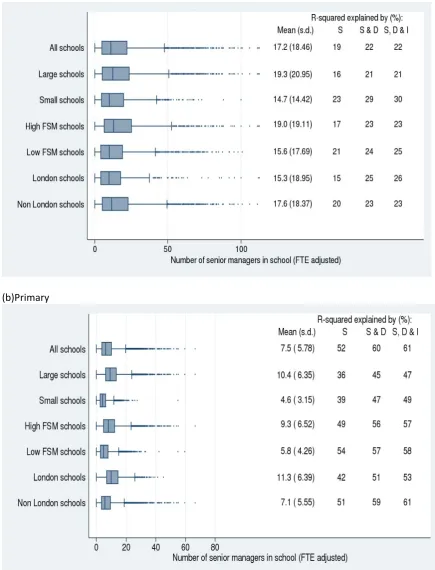
Variation in senior management deployment

(22)

(23)

Part

2:

How

is

the

‘residual’

income

that

some

schools

receive

spent?

A different way of conceptualising schools’ discretion in spending is to consider how they spend the income that they have that is not accounted for by their circumstances. We describe this as their ‘residual’ income but it could equally be called unexpected income since the typical ‘like’ school does not receive this money. One reason that this residual income might be interesting is that it might tell us something about the marginal decisions schools make about spending their last pounds. So, it might help us understand what happens if a school is given a little extra money.

We calculate residual income by regressing each school’s total income on the structural and demographic characteristics defined above, and extracting the residual from the regression

estimates. We then regress each expenditure item we defined above on this residual income and all the structural and demographic characteristics defined above. In each regression we use the

coefficient on residual income as a measure of how the extra pound of income is spent. As we noted, this exercise is similar to comparing the impact on the R2 of adding income to the regressions above, but here we focus on which items see the greatest change in expenditure.

Table 1 column A presents the results of the relationship between residual income and expenditure items in secondary school. For each expenditure item, we present in the table the coefficient on residual income, the estimated standard error and the R2. The remainder of the coefficients are not presented.

The top row – for total expenditure – has a coefficient close to 1, as it should have. This implies that almost all the residual income that is given to a school is spent in that year. Many other expenditure items have estimates close to zero, but the items with substantial and significant coefficients are:

Expenditure on teaching staff where the coefficient is 0.2, meaning that for every £1 of residual income a school gets, they spend about 20p on teaching staff;

Expenditure on educational support where the coefficient is 0.08 or 8p in every £1 of residual income received;

Expenditure on classroom teachers in the SWC has a coefficient of 0.1 implying that only 10p in a £1 of residual income is spent on classroom teachers;

Expenditure on senior management in the SWC has a coefficient of 0.01 implying that only 1p in £1 is spent here (though note our concerns about data quality);

School‐level pay premium coefficient is 0.29, suggesting that about a third of the residual income is associated with a higher pay premium in the school.

The pay of the Headteacher coefficient is 1.9. Taken literally, this means that more than the extra is spent on the Headteacher’s salary. However, these regressions are not intended to be understood as causal, they simply measure association. For example, it could be in part that highly paid

(24)

Table 1 column B presents the same analysis for primary schools. We see a similar pattern here, though with some interesting differences. The more substantial coefficients are:

Expenditure on teachers (0.32)

Expenditure on education support (0.18)

Expenditure on classroom teachers in the SWC (0.13)

Expenditure on senior management (0.07)

The pay of the Headteacher (1.38)

School‐level pay premium (0.28).

In both cases, the pay of the Headteacher is the most highly associated with the residual income.

Part

3:

Where

income

changes

between

two

years,

how

is

it

spent?

We compared school income and expenditure in 2008/9 and 2009/10. Only a few schools see stable income; for example, only 11% of schools experienced an absolute change in income of less than 1%, while 22% saw a fall in income and 61% had a rise greater than 5% (all in nominal terms). We are not chiefly concerned about how or why the income increased, but we will use the CFR data to analyse how the change is deployed. Note that as we only have one SWC, we can only consider changes in the CFR data. This analysis relates only to secondary schools.

To make things manageable we group the CFR expenditure items as follows:

• Group 1, "Teachers": Teaching staff costs

• Group 2, "Ed Support": Education support staff costs

• Group 3, "Other staff and staff‐related": Supply staff costs, Premises staff costs, Administrative and Clerical staff costs, Catering staff costs, Costs of other staff, Indirect employee expenses, Development and training costs, Supply teacher insurance costs, and Staff related insurance costs.

• Group 4, "Buildings related": Building maintenance and improvement costs, Grounds

maintenance and improvement costs, Cleaning and caretaking costs, Water and sewage costs, Energy costs, Non domestic rates expenditure, and Other occupation costs.

• Group 5, "Learning and ICT resources": Learning resources costs (not ICT equipment)and ICT Learning resources costs.

• Group 6, “Other”: Exam Fees, Administrative supply costs, Other insurance premiums, Special facility costs, Catering supply costs, Agency supply teaching staff costs, Bought professional services – curriculum, Bought professional services – other, Community focused extended school staff and Community focused extended school costs.

• Group 7, “Balance”: Total income minus total expenditure

(25)

(26)

(27)

schools and to use policy briefings to disseminate best practice. We believe there are a number of problems with this approach and suggest how a behavioural economics approach might be capable of improving school financial decisions.

Difficulties

with

current

policy

approach

of

dissemination

of

best

practice

The current approach to helping schools make efficient financial decisions consists of a two‐fold approach of benchmarking and best practice advice. The DfE School Financial Benchmarking website2 allows schools to compare their CFR returns to those of similar schools across the country to see where their own spending is significantly different from peers. However, the website’s usefulness to schools is clearly limited because it cannot disaggregate teaching staff expenditure between management and classroom teachers, and is silent on which of these comparison schools is a successful school. The website does not allow users to easily relate these high level expenditure data to school outcomes. It is therefore an inadequate tool for giving any explicit advice on best practice on spending patterns. Perhaps this lack of directed advice explains why only a minority of headteachers and managers have ever accessed this website; in a sample of 38 schools, Dodd (2008, p. 38) finds that: “Few of the schools take a genuine interest in or see much value in benchmarking their performance using either parent local authority data or the DfES benchmarking web‐site. This is slightly surprising as one of the characteristics of the sample schools is a refusal to accept that current levels of performance cannot be improved.” The DfE reports that usage has picked up in more recent years (2010‐11). There are many sources of ideas available to schools on how to spend their money (although some are more firmly backed by evidence than others), in the UK and further afield3. Some recent examples which are based on analysis include a series of briefs released by the Audit Commission (2011a, 2011b, 2011c, 2011d) outlining potential areas for cost savings and efficiencies. The reports covered areas including classroom deployment, the curriculum, and managing staff absence and cover. Although the reports suggested there were many areas in which savings may be made, the authors concluded most areas held limited scope for cost reduction and suggested better utilisation of teaching assistants was the area which may hold the most scope for savings. In a second example, the Sutton Trust released detailed guidance (Higgins et al, 2011) on “how to spend the pupil premium”, which cited research findings. The document listed possible choices with an evaluation of the likely impact on test scores and the cost effectiveness. These guidance documents on best practice are necessarily limited by the lack of a strong and robust evidence base from which we can specify what best practice is, either in general or varying with circumstances. This is a serious impediment to improving schools’ financial decisions. As we noted above, while it seems unlikely that the patterns of substantial and largely idiosyncratic variation we see are optimal decisions, there is no agreed and well‐supported view of what would be optimal. 2_{http://www.education.gov.uk/sfb}

(28)

The lack of any firm recommendations at an aggregate is compounded by the fact that schools do face very different operational environments. The quality of instruction and a school’s climate are complex and abstract. Whereas centralized systems are good at imparting simple spending rules, it is not obvious that remotely‐designed rules are effective in dealing with complex resource use. Government agencies do have a role in facilitating analysis of aggregated schools’ data and implementing careful studies, both of which should influence understanding on best practice. However, they are likely to be less good at understanding that complex resource development is necessarily sensitive to specific contexts, so the learnt experiences of schools will always be critical. ‘‘Bottom‐up’’ development of knowledge in this way also holds the potential of substantial long‐run productivity growth through radical innovation at schools. Furthermore, teachers may respond more positively to a system that empowers them to make choices rather than imposes restrictions.

Using

behavioural

economics

to

help

improve

financial

decisions

The behavioural economics tradition is well suited to analysing how to encourage headteachers and financial managers to take a more proactive role in improving school efficiency. Interestingly, Dodd (2006) reports that the majority of headteachers believe their school is efficient, but this seems unlikely giving that many heads devolve school resource planning to bursars who simply produce budgets based on rolling‐forward historical expenditure.

Dolan et al (2010) characterise the innovations provided by behavioural economics as: “Drawing on

psychology and the behavioural sciences, the basic insight of behavioural economics is that our

behaviour is guided not by the perfect logic of a super‐computer that can analyse the cost‐benefits of

every action. Instead, it is led by our very human, sociable, emotional and sometimes fallible brain.” It is now clear that we make decisions in two ways: reflective and automatic (see Thaler and Sunstein, 2008). The first is what traditional economics focuses on and we described towards the start of this report, based on information, constraints and incentives. The second is based on more immediate stimuli and reflects much more automatic and seemingly irrational and inconsistent decisions. It has been described as “changing behaviour without changing minds”. There is a difficulty here, mentioned above, in that the research base does not provide a “best allocation” that we can use the tools of behavioural economics to ‘nudge’ people towards. Unlike, for example, in trying to affect obesity, there is no obvious best behaviour to adopt. The goal instead has to be to get schools to be more reflective and thoughtful in deciding their spending patterns. This trend towards encouraging schools to think more about spending is evident in the School Financial Benchmarking website. Here we make five suggestions (drawing on Dolan et al., 2010) as to how behavioural economics can help take this approach further:

1. Get the right messenger

The reception that people give a message, such as suggestions on school spending, depends on the nature of the messenger. People are generally more open to information from others with

demographic and behavioural similarities, and who are credible experts. This suggests that

(29)

practice. However, where a school is required to cut its budget, the headteacher of the very similar school that already operates on the lower budget is a credible expert in how this is achievable.

2. Give explicit incentives for schools to save money

The current financial system for schools offers no incentives to save money. Indeed, for local authority maintained schools it is important to spend all income received to avoid the budget being reduced in future years. While there are reasonably important incentives for improving outcomes (via school performance tables etc), they are rather distant from the financial decisions – and may even be disconnected in the minds of school leaders. While we do not want to encourage a ‘race to the bottom’ to provide the cheapest education possible, school governors might be encouraged to offer bonus payments to headteachers and financial managers under certain circumstances. One situation might be where a school is identified as having higher costs than other schools in identical structural and demographic circumstances, and so a share of any cost reduction achieved could be passed to school leaders in bonus payments. Another situation where bonus payments might be appropriate is where a school is running a deficit and so has little option but to reduce costs. It may sound counterintuitive to pay bonuses in this situation, and would be politically difficult in a time of austerity, but by aligning the incentives of school leaders and governors it may encourage difficult or even innovative cuts to be made.

3. Schools are attracted to following typical behaviour or norms

School ought to be interested in what other schools do, and reporting positive norms has been found to encourage individuals in achieving desirable outcomes. Once again, our problem is a lack of understanding as to what constitutes best practice in schools. However, encouraging high cost schools (given their circumstances) to explore data on spending in similar schools is likely to improve the efficiency of the system overall. This may not happen automatically because the benchmarking website is not currently very heavily used. One approach could be to use data to identify schools with unexpectedly high costs and pro‐actively transmit with information to their school leadership teams, with the requirement that they be considered by school governors. All schools could also be encouraged to carry out routine “waste audits” to see whether funds are being spent inefficiently (see for example, Grubb and Tredway, 2010, and the Audit Commission, 2009). Clearly, these suggestions rely somewhat on traditional regulation rather than behavioural nudges.

4. Prevent rolling forward historical spending being the default budget plan

(30)

school’s own data. This has dangers of course: showing the average for comparator schools may undermine a high performing school doing something very well.

5. Nurture the self‐image of headteachers as outstanding financial managers

(31)

References

Aaronson, D., Barrow, L., & Sander, W. (2007). ‘Teachers and student achievement in the Chicago Public High Schools’, Journal of Labor Economics, 25(1), 95–136.

Angrist, J. and Lavy, V. (2002). ‘New evidence on classroom computers and pupil learning’, Economic

Journal, vol. 112, pp. 735–65.

Audit Commission (2004), Education Funding: The Impact and Effectiveness of Measures to Stabilise

School Funding, London.

Audit Commission (2009). Valuable lessons: Improving economy and efficiency in schools, Briefing for head teachers and school staff with financial responsibilities. Retrieved from http://www.audit‐

commission.gov.uk/SiteCollectionDocuments/AuditCommissionReports/NationalStudies/valauable

lessonsteachersguide30June2009.pdf

Audit Commission (2011). Better value for money in schools: Classroom deployment

http://www.audit‐

commission.gov.uk/localgov/audit/childrenandyoungpeople/Pages/bettervalueformoneyinschools.a spx

Audit Commission (2011). Better value for money in schools: Curriculum breadth http://www.audit‐

Audit Commission (2011). Better value for money in schools: The wider school workforce

http://www.audit‐

Audit Commission (2011). Better value for money in schools: Managing staff absence and cover

http://www.audit‐

Blatchford, P., Russell, A., Bassett, P., Brown, P., Martin, C (2007) ‘The role and effects of teaching assistants in English primary schools (Years 4 to 6) 2000‐2003. Results from the Class Size and Pupil‐ Adult Ratios (CSPAR) KS2 Project’, British Educational Research Journal, Volume 33, Number 1, pp. 5‐ 26

Chetty, R., Friedman, J., Hilger, N., Saez, E., Whitmore Schanzenbach, D., and Yagan, D. (2010) How Does Your Kindergarten Classroom Affect Your Earnings? Evidence From Project STAR, NBER Working Paper No. 16381.

(32)

Dearden, L., Ferri, J. and Meghir, C. (2002), ‘The effect of school quality on educational attainment and wages’, Review of Economics and Statistics, vol. 84, pp. 1–20

Department for Education (2011), Improving efficiency in schools, retrieved from

http://media.education.gov.uk/assets/files/pdf/i/improving%20efficiency%20in%20schools.pdf

Dodd, A. (2006), Investigating the effective use of resources in secondary schools, DCSF Report No. RR799. Retrieved from DfES website:

http://www.education.gov.uk/research/data/uploadfiles/RR799.pdf.

Dolan, Paul and Hallsworth, Michael and Halpern, David and King, Dominic and Vlaev, Ivo (2010). MINDSPACE: influencing behaviour for public policy, Institute of Government, London, UK. Dolton, P., & Van der Klaauw, W. (1999). ‘The turnover of UK teachers: A competing risks explanation’, Review of Economics and Statistics, 81(3), 543–552.

Dustmann, C., Rajah, N. and van Soest, A. (2003), ‘Class size, education, and wages’, Economic

Journal, vol. 113, pp. F99–120.

Feinstein, L., & Symons, J. (1999). ‘Attainment in secondary school’, Oxford Economic Papers, 51, 300–321

Fuchs, T. and Woessmann, L. (2004). Computers and Student Learning: Bivariate and Multivariate

Evidence on the Availability and Use of Computers at Home and at School, CESifo WP 1321 Goolsbee, A. and Guryan, J. (2006). _’The impact of internet subsidies in public schools’, Review of

Economics and Statistics, vol. 88(2), pp. 336–47.

Grubb, W. N. (2010). Moving research into practice: Creating an educational extension service, Unpublished manuscript.

Grubb, W. N., & Tredway, L. (2010). Leading from the inside out: Expanded roles for teachers in

equitable schools. Boulder, CO: Paradigm Press.

Grubb, W.N. and Allen, R. (2011) ‘Rethinking school funding, resources, incentives, and outcomes’, Journal of Educational Change, 12(1)121‐130

Hanushek, E. A. (1986). ‘The economics of schooling: production and efficiency in public schools’;

Journal of Economic Literature, vol. 24 (September), pp. 1141–77

Hanushek, E. A. (1989). ‘Expenditures, efficiency, and equity in education: the federal government’s role’, American Economic Review, vol. 79(2), pp. 46–51.

Hanushek, E. A. (1996). ‘A more complete picture of school resource policies’; Review of Educational

Research, vol. 66, pp. 397–409.

(33)

Hanushek, E. A. (2003). ‘The Failure of Input‐based Schooling Policies’; The Economic Journal, Vol 113, Issue 485, Pages F64‐F98

Hanushek, E. A. (2004). ‘What if there are no ‘Best Practices’’, Scottish Journal of Political Economy, Volume 51, Issue 2, pages 156–172

Hanushek, E. A. (2010). ‘The Economic Value of Higher Teacher Quality’, Economics of Education

Review, Volume 30, Issue 3, June 2011, Pages 466‐479

Higgins, S., Kokotsaki, D. And Coe, R. (2011) Toolkit of Strategies to Improve Learning: Summary for Schools Spending the Pupil Premium. Sutton Trust.

Holmlund, H., McNally, S. and Viarengo, M. (2008), Impact of School Resources on Attainment at Key

Stage 2, DCSF Research Report no. RR043, London: Department for Children, Schools and Families.

Jenkins, A., Levačić, R. and Vignoles, A. (2006), Estimating the Relationship between School Resources

and Pupil Attainment at Key Stage 3, London: Department for Children, Schools and Families. Kane, T., Taylor, E., Tyler, J. and Wooten, A (2010), Identifying Effective Classroom Practices Using

Student Achievement Data, NBER WP w15803

Krueger, A. B. (2003) ‘Economic considerations and class size’, The Economic Journal, 113 (February), F34–F63

Krueger, Alan B., and Diane M. Whitmore, (2001) ‘The Effect of Attending a Small Class in the Early Grades on College‐Test Taking and Middle School Test Results: Evidence from Project STAR’, The

Economic Journal, 111 (2001), 1‐28.

Lavy, V. (2011). What makes an effective teacher? Quasi‐experimental evidence, Hebrew University of Jerusalem Unpublished

Leuven, E., Lindahl, M., Oosterbeek, H. , and Webbink, D. (2004), The Effect of Extra Funding for

Disadvantaged Pupils on Achievement; IZA Discussion Paper, 1122.

Levačić, R., Jenkins, A., Vignoles, A., Steele, F. and Allen, R. (2005), Estimating the Relationship

between School Resources and Pupil Attainment at Key Stage 3, DCSF Research Report no. RR727, London: Department for Children, Schools and Families.

Machin, S., McNally, S., and Meghir, C. (2007a). Resources and Standards in Urban Schools, Centre for the Economics of Education DP 76

Machin,S., McNally, S., Silva, O. (2007b). ‘New Technology in Schools: Is There a Payoff?’; The

Economic Journal , Volume 117, Issue 522, pages 1145–1167

Rivkin, S. G., Hanushek, E. A., & Kain, J. F. (2005). ‘Teachers, schools and academic achievement’, Econometrica, 73(2), 417–458.

Schanzenbach, Diane W., ‘What Have Researchers Learned From Project STAR?’, Brookings Papers

(34)

Slater, H., Davies, N. and Burgess, S. (2009), Do teachers matter? Measuring the variation in teacher

effectiveness in England, Centre for Market and Public Organisation (CMPO), Working Paper no.

09/212

Sunstein, C and Thaler, R (2008). Nudge: Improving Decisions About Health, Wealth and Happiness. Yale: Yale University Press

Wild, R., Munro, F., & Ayoubkhani, D. (2009). Public service output, input and productivity:

Education, Working Paper no. 09/212. Retrieved from Office for National Statistics website: http://www.statistics.gov.uk/articles/no journal/education‐productivity.pdf

(35)

Fig.1 Box‐graph showing the variation in total income per pupil (a) Secondary

(b) Primary

[image:35.595.68.504.98.661.2]

(36)

Fig.2 Box‐graph showing the variation in total expenditure per pupil (a) Secondary

(b) Primary

Note: Data on dependent variable from CFR

[image:36.595.69.503.100.613.2]

(37)

Fig.3 Box‐graph showing the variation in total expenditure on teachers per pupil (a) Secondary

(b) Primary

[image:37.595.69.502.119.698.2] [image:37.595.73.498.416.699.2]

(38)

(b) Primary

[image:38.595.72.500.72.650.2]

(39)

(b) Primary

Note: Data on dependent variable from SWC

[image:39.595.72.501.71.655.2]

(40)

(b) Primary

[image:40.595.70.523.70.646.2]

(41)

(b)Primary

[image:41.595.70.506.70.641.2]

(42)

(b) Primary

[image:42.595.72.499.72.645.2]

(43)

(b) Primary

[image:43.595.72.498.181.637.2]

(44)

(b) Primary

[image:44.595.70.503.69.641.2]

(45)

(b) Primary

[image:45.595.69.500.74.640.2]

(46)

(b) Primary

[image:46.595.71.499.72.646.2]

(47)

(b) Primary

(48)

Fig.14 Box‐graph showing the variation in proportion of teachers with qualification in main

teaching subject

Note: Data on dependent variable from SWC (secondary schools only)

Fig.15 Box‐graph showing the variation in proportion of maths teachers with qualification in maths

[image:48.595.73.500.100.365.2] [image:48.595.72.498.421.673.2]

(49)

Fig.16 Box‐graph showing the variation in proportion of English teachers with qualification in

English

Fig.17 Box‐graph showing the variation in proportion of science teachers with qualification in

science

[image:49.595.73.501.98.377.2] [image:49.595.73.498.448.718.2]

(50)

Fig.18 Box‐graph showing the variation in generosity of teacher pay (a) Secondary

(b) Primary

[image:50.595.69.502.106.657.2]

(51)

Figure 19: Details of the variation in percentage change in expenditure on different categories across the quintiles of income growth

[image:51.595.71.640.91.489.2]

(52)

[image:52.595.74.633.102.496.2]

(53)

[image:53.595.74.486.88.746.2]

Figure 21: Expenditure category change against Income change

(54)

Table 1: Relationship between Residual Income and Expenditure

Secondary Schools Primary Schools

Coeff (SE) R‐sqd No. Of obs Coeff (SE) R‐sqd

No. Of obs

Expenditure total 0.886 (0.009) 0.941 2680 0.949 (0.004) 0.939 12994 Expenditure teachers 0.204 (0.008) 0.710 2680

0.325 (0.004) 0.735 12592 Expenditure support 0.082 (.005) 0.571 2680 0.184 (0.003) 0.638 12592 Teaching assistant ‐0.005 (.005) 0.687 81 0.000 (0.001) 0.500 335 Teacher expenditure 0.102 (0.015) 0.769 2585 0.129 (0.005) 0.226 12690 Senior management expenditure 0.008 (0.012) 0.184 2534 0.073 (0.003) 0.508 12832 Number of managers 0.001 (0.001) 0.215 2680 0.001 (0.000) 0.601 12994 Age of young teachers 0.000 (0.000) 0.202 2680 ‐0.001 (0.000) 0.096 12983 Proportion with QTS 0.000 (0.000) 0.173 2674 ‐0.000 (0.000) 0.061 12978 Non‐teacher permanent staff 0.000 (0.000) 0.054 2676 0.001 (0.000) 0.061 12974 Short tenured 0.000 (0.000) 0.054 2680 ‐0.000 (0.000) 0.045 12983 Age of Head teacher 0.000 (0.000) 0.051 2581 0.000 (0.000) 0.019 12486 Pay of Head teacher 1.927 (0.447) 0.385 2522 1.384 (0.104) 0.595 12375 Teacher relative pay 0.288 (0.065) 0.505 2628 0.276 (0.065) 0.509 11934 Qualification main subject 0.000 (0.000) 0.164 2125

[image:54.595.76.619.71.389.2]

(55)

Table 2: Change in total school income and expenditure items

Mean % Change in Expenditure on: Quintiles of %

Change in Total Income

Mean % Change in

Total Income Teachers Ed Support

Other staff and staff‐

related

Buildings related

Learning and ICT

resources Other Balance

Largest fall ‐3.675 ‐0.206 0.519 ‐0.484 ‐0.484 ‐0.923 ‐0.393 ‐1.598 2 1.227 1.296 0.765 ‐0.13 ‐0.23 ‐0.396 0.096 ‐0.281 3 3.688 2.076 0.834 ‐0.021 ‐0.159 ‐0.213 0.452 0.753 4 6.166 2.442 0.955 0.178 0.072 0.333 0.701 1.432 Highest rise 12.172 3.719 1.183 0.453 1.226 0.912 1.843 2.913

[image:55.595.67.742.83.231.2]

(56)

Table 3: What items school change the most:

(a) Percentage of schools for which each item had the highest increase in expenditure

Percentage of schools for which this item had the highest increase in expenditure:

Quintiles of % Change in

related

Learning and

ICT resources Other Balance N

Largest fall 27.85 15.7 7.85 6.58 7.34 16.71 17.97 395

2 41.06 12.74 4.42 5.84 6.02 11.86 18.05 565

3 48.71 6.83 2.58 3.69 5.9 8.67 23.62 542

4 46.36 7.51 1.99 3.53 7.95 9.05 23.62 453

Highest rise 41.37 2.16 1.8 7.19 8.27 12.59 26.62 278

Total 41.69 9.45 3.76 5.15 6.9 11.46 21.59 2233

(b) Percentage of schools for which each item had the biggest fall/lowest rise in expenditure

Percentage of schools for which this item had the biggest fall/lowest increase in expenditure:

Quintiles of %

Change in

related

Learning and

ICT resources Other Balance N

Largest fall 19.49 1.27 8.1 9.11 18.23 12.15 31.65 395

2 9.03 2.83 10.97 15.4 21.59 10.62 29.56 565

3 4.24 2.03 14.76 18.27 26.75 11.99 21.96 542

4 3.09 4.19 18.32 19.65 20.09 17.88 16.78 453

Highest rise 4.68 4.32 18.35 22.66 22.66 13.31 14.03 278 Total 7.97 2.82

Understanding school financial decisions

Research Report DFE-RR183

Rebecca Allen, Institute of Education, University of London

Contents

Executive

Results

Results

Review

Class

Teacher

Teaching

Resources

National

Consistent

Detailed

schools?

Variation in total income and expenditure

Variation in senior management deployment

‘residual’

Where

Difficulties

Using

1. Get the right messenger

3. Schools are attracted to following typical behaviour or norms

References

Fig.14 Box‐graph showing the variation in proportion of teachers with qualification in main

English

Secondary Schools Primary Schools

Mean % Change in Expenditure on: Quintiles of %

Percentage of schools for which this item had the highest increase in expenditure:

Percentage of schools for which this item had the biggest fall/lowest increase in expenditure: