Comparison of Classifier Strength for Detection of Retinal Hemorrhages

ISSN: 2278-3075, Volume-8, Issue-6S3, April 2019

Abstract: Diabetes Mellitus(DM) which is the root cause of diabetic retinopathy(DR) diseases such as occlusion, microaneurysms, retinal hemorrhage, etc. Hemorrhage is considered the most dangerous among these, as it can accelerate the occurrence of vision loss. Hence, the severity of hemorrhages is analyzed in most of the recent studies of diabetic retinopathy detection. This paper focusses on the best classification approach by comparing different machine learning approach using supervised classifiers. Fundus image collected from publically available database are preprocessed and enhanced. Using splat based method, ground truth is established with the help of a retinal expert. Supervised classifiers are trained from the GLCM features extracted from the segmented images and validated on clinical images. The experimental results were verified by the Area Under Curve(AUC) for the three classifiers that were trained and results are verified and tabulated.

I. INTRODUCTION

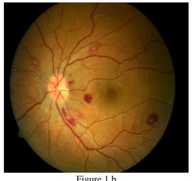
DR detection is usually done from the analysis of fundus images. The fundus image of a person with the retinal hemorrhage compared with a normal retina is shown in Fig. 1. Image segmentation is the technique used to extract the features and analyze retinal images. This method is non-invasive and cost effective and that is the reason we chose Image based method for our analysis.

Figure 1 a

Figure 1 a. Fundus Image of a Normal Retina.

Sreeja K.A., Asst. Professor, Dept. Of Electronics and Communication Engg., SCMS School of Engineering & Technology, Karukutty, Ernakulam, Kerala, India. ([email protected])

S.S. Kumar, Associate Professor, Dept. of Electronics and Instrumentation Engg., Noorul Islam University, Kanyakumari, Tamil Nadu, India.

Figure 1 b

Figure 1 b. DR Fundus image with Hemorrhages.

II. LITERATURE REVIEW

Recent developments in DR studies suggest an increase in the number of diabetic patients as well as new methods to detect the retinopathy symptoms like retinal hemorrhage. A systematic review has been described using PRISMA guidelines in [1] based on meta-analysis. IN order to discern between DR and glaucoma Rommel et. al [2] proposed a work using statistical texture analysis for retinal disease screening. The implementation of a digital tool that facilitates ophthalmologist to what extent the DR has affected is proposed in [3]. The implementation is based on Gabor transform and uses digital filters for a quality retinography tool. Detection of all the DR symptoms such as Microaneurysms, exudates, hemorrhages, etc. has been reviewed in [4]. Alongside several blood vessel detection technique for retinal fundus images have been described in [4].Recent studies on Diabetic Neuropathy is presented by R. B. Kakkeri. et. al. [5] where the phenomenon called neovascularization is explained. Machine learning algorithm based retinopathy diagnosis in [6] predicts the presence of diabetic retinopathy using alternating decision tree, adaBoost, Naive Bayes, Random Forest and SVM classifiers. Exudate detection using artificial neural network algorithm was presented in [7].

III. FUNDUS IMAGE SEGMENTATION

Image segmentation techniques, as already said is the effective method to extract features from a retinal fundus image. There are several image segmentation techniques

available over literature which

Comparison of Classifier Strength for

Detection of Retinal Hemorrhages

can be utilized to segment the required region in an image. All segmentation methods share some of the common stages, such as pre-processing, processing and post-processing stages. Retinal segmentation techniques are broadly classified into two [8] as rule based methods and machine based methods. In this paper, machine based methods are preferred that utilizes ground truth and has a labelled dataset to train the classifiers. An irregular segmentation technique employing a high level entity called splat is the method[9] utilized here. Pixels that share the same structural and spatial properties are partitioned into a non-overlapping entity known as splat. Since, Hemorrhages contain blood, those hemorrhage pixels have similar properties such as color, intensity, spatial locations etc. These pixels are delineated from the whole image to form hemorrhage splats. Before segmentation of the fundus image to generate splats, the blood vessels are to be removed so that the they should not be misinterpreted as hemorrhages since both have similar structural properties.

III a.Blood vessels removal

Inorder to make the splat based method more effective, the blood vessels are removed using a Kirsch compass kernel. [10]The Kirsch’s operator takes a single kernel mask and turns it in 45 increments over all 8 compass courses such as: N, NW, W, SW, S, SE, E, and NE. The maximum magnitude across all directions is the value of edge magnitude of the Kirsch operator. It is calculated as

ℎ𝑛,𝑚= max

𝑧=1,…8∑ ∑ 𝑔𝑖,𝑗

(𝑧)

. 𝑓𝑛+𝑖,𝑚+𝑖 1

𝑗=−1 1

𝑖=−1

(1)

Where 𝑔𝑧 _{is the 8 different compass direction kernels.}

III b. Splat Generation

Using edge detection, the vessels are delineated and the image is segmented to generate splats. Meaningful splats, are created by a scale specific over segmentation which is done in two steps. Initially, gradient scale of contrast enhanced bright-dark opponent image is taken using diverse gradations(scales), as the appearance of hemorrhages varies in different locations. The values of the scales are grouped and the highest of the gradient value with its scale of interest(SOI) is taken to accomplish watershed segmentation. [11]

The gradient magnitude is computed using the equation

|∇𝐼(𝑥, 𝑦; 𝑠)|

= √𝐼𝑥(𝑥, 𝑦; 𝑠)2_{+ 𝐼}

𝑦(𝑥, 𝑦; 𝑠)2

(2)

where 𝐼(𝑥, 𝑦; 𝑠) is the image. Now creating a scale-space depiction of the image using Gaussian kernels 𝐺𝑠, the gradient magnitude is computed from its derivatives –the horizontal and vertical ones as:

|∇𝐼(𝑥, 𝑦; 𝑠)|

= √[𝜕

𝜕𝑥(𝐺𝑠∗ 𝐼(𝑥, 𝑦))] 2

+ [𝜕

𝜕𝑦(𝐺𝑠∗ 𝐼(𝑥, 𝑦))] 2

(3)

|∇𝐼(𝑥, 𝑦; 𝑠)|

= √[𝜕𝐺𝑠

𝜕𝑥 ∗ 𝐼(𝑥, 𝑦))] 2

+ [𝜕𝐺𝑠

𝜕𝑦 ∗ 𝐼(𝑥, 𝑦))] 2

(4)

where the symbol ∗ signify convolution and 𝜕𝐺𝑠 𝜕𝑥 and

𝜕𝐺𝑠 𝜕𝑦 are the 1 derivatives of Gaussian in the x axis and y axis direction using the scale s

The highest of the gradient magnitude is

|∇𝐼(𝑥, 𝑦)| = max

𝑖 |∇𝐼(𝑥, 𝑦; 𝑠𝑖)| (5) While the field surface in watershed algorithm is essential [11] to attain meaningful splats, the greatest of the gradient magnitude is taken for a definite scale of Interest (SOI). The splats are generated based on Algorithm 1.

Algorithm 1. Splat Generation 1:

2: 3: 4: 5: 6: 7: 8: 9: 10: 11: 12: 13: 14: 15: 16:

function SPLAT_GEN(gradientoutputimage)

nSeg  Number of segments required

thresGrad  Gradient threshold

top:

finSeg  Number of segments generated after watershed segmentation

if nSeg > finSeg then

thresGrad  thresGrad+1 loop:

ifimageGrad(a)(b) > thresGrad then

newimageGrad(a)(b)  imageGrad(a)(b) p=a+1

q=b+1 goto loop.

imageGrad = newimageGrad

gototop.

returnfinalimage  watershed(imageGrad)

Thus the image can be portioned as non-overlapping splats having similar intensity over the entire image[9]. Some of the Splats formed by means of diverse scales exploiting the same watershed algorithm is shown in the figure 2.

ISSN: 2278-3075, Volume-8, Issue-6S3, April 2019

Figure 2b

Figure 2c

Fig. 2a has smaller splats which are generated with scales outside the desired SOI for hemorrhage splats. The range of scales used in Fig. 2a can be used for optic disc removal and blood vessel detection. Fig. 2b uses a fine scale and also less than the desired SOI. These range of scales can be used in the detection of Microaneurysms and exudates. Figure 2c is the required scale for hemorrhages detection as the retinal background is represented by larger splats and blood regions are represented as smaller splats.

The total number of splats generated is kept under a threshold without compromising the accuracy and speed of computation.

IV. GOLD STANDARD LABELLING BY

OPHTHALMOLOGIST

The splats obtained by segmentation are labelled with the help of an ophthalmologist in order to train the supervised classifiers for the clinical images. For the DIARETDB1 database, ground truth’s confidence level is kept as 0.75 based on the evaluation done in [12].This level is the certainty of the decision that a splat is accurate.

Feature Extraction and Feature Subset Selection:

The classifiers can be trained to detect the target objects after assigning reference labels for splats. An overall 352 possibly relevant features are taken from each splats to train the classifiers.

They are:

1)Color: Colors of each splat is obtained in RGB color space and dark-bright (db), red-green (rg), and blue-yellow (by) opponency images [13], which derives to six colour components.

2) Difference Of Gaussian (DoG Filter ): Difference of Gaussian (DoG) kernels are employed at five distinct

smoothing scales with one baseline scale to take advantage of Gaussian scale space. [14][15]

3) Responses from Gaussian Filter Bank[13]: A Gaussian filter bank which include a first order derivative and a second order derivative with at two orientations and three orientations respectively are applied to the green channel.

4)Responses from Schmid Filter Bank: 13 kernels of Schmid filter banks which are rotationally invariant is applied to the dark bright opponency image.

5)Responses from Local Texture Filter Banks: Local texture filter bank contains local entropy filter, local range filter and local standard deviation filter which calculate the entropy, standard deviation and intensity range of a single pixel in a given region [16].

The above features are combined to obtain a meaningful response image that has small inter splat similarity and large intra splat similarity[13] [15] [16] [17]. These features mentioned above are called pixel- based responses. Alongside these features, we take splat wise features according to Gray-Level Co-occurrence Matrix (GLCM)[16] [18] [19] [20]statistics. These are splat area, extent, texture, solidity and orientations. After sequential forward feature selection subset(SFS) insignificant and redundant ones were removed from the feature set and only the relevant features were considered. The 19 features considered for training the classifiers are shown in Table I

TABLE I

Features Number Description

DoG filter bank DoG filter bank DoG filter bank

Gaussian Filter Bank

Gaussian Filter Bank

Schmid filter bank

Mean of

Gaussian

s2 - s0.5 s4 - s0.5 s8 - s 0.5

s=8

orientation:2,3

s=1,2,4

orientation:1,2,3

response=11 s=8,16

from Green channel from db and rg opponency

from db opponency

Mean of second order Gaussian derivative from green channel

Mean of second order Gaussian derivative from green channel

from db opponency from Green channel

V. CLASSIFICATION USING DIFFERENT CLASSIFIERS

In order to do the classification, several machine learning algorithms are available over literature. Among them, three classifiers are used to train our experiment and evaluate the result. They are: Neural Network Classifier, Naïve Bayes Classifier and kNN Classifier.

A. Neural Network classifier:

human brain forms the key part of a neural network. Individually nodes have their own scope of intelligence concerning rules and functionalities to improve it-self through knowledges learned from previous methods which is called backpropagation. Neural networks are suitable to identify non-linear patterns, where there isn’t a one-to-one relationship between the input and output[21]. The neural network consists of input layers, hidden layers and a threshold function. All the nodes are interconnected to form a network.

Neural networks are characterized by holding adaptive weights along paths between neurons that can be adjusted by a backpropagation algorithm that learns from perceived data in order to improve the learning model The inputs to the neural network classifier are the relevant feature set and they are transformed using the desired weights from the hidden layer. Finally, using a sigmoid transfer function the output class is determined.

B. Naïve Bayes Classifier:

The naive Bayes classifier [22]uses the principle of Bayesian maximum a posteriori (MAP) classification: measure a finite set of features 𝑥 = (𝑥1, … . . , 𝑥𝑛) then select the class

𝑦̂ = 𝑎𝑟𝑔 max 𝑦 𝑃(𝑦|𝑥)

where

𝑃(𝑦|𝑥)𝑃(𝑥|𝑦)𝑃(𝑦)

(6)

𝑃(𝑦|𝑥) is the likelihood of feature vector x given class y, and 𝑃(𝑦) is the priori probability of class y. Naive Bayes classifier assumes that the features are independent of the condition. For the class:

𝑃(𝑦|𝑥) = ∏ 𝑃(𝑥𝑖|𝑦) 𝑖

(7)

The parameters 𝑃(𝑥𝑖|𝑦) and 𝑃(𝑦) are obtained from the training data.

C. kNN Classification

The kNN algorithm allocates soft class labels. The two output classes defined are hemorrhage splat or non-hemorrhage splat. Euclidean distance is the measure by which the classifier decides whether a particular splat belongs to hemorrhage or normal class in an optimized feature space. As the value of k is increased the computation time increases and the splats are more accurately identified. But since all the k nearest neighbors are not near, an optimum value of k is chosen instead of an arbitrary value.

VI. EXPERIMENT AND RESULTS

A. Data acquisition and Pre-processing

The fundus images were acquired from two sources. Clinical images were obtained from Dr. Bhejan Singh’s eye hospital. The clinical image was captured using a “Remidio Non-Mydriatic Fundus On Phone (FOP-NM10)”

[23]Camera with FOV 40, working distance of 33mm and an ISO range from ISO 100 to 400. The images used for training was acquired from the publically available database DIARETDB1

(http://www.it.lut.fi/project/imageret/diaretdb1/index.html).

An overall 1500 images were taken among which 1050 images were taken for training, 225 images for testing and 225 for validation. The gold standard reference observations were accomplished by an ophthalmologist expert using the splat-based interpretation. Overall 1200 (950 from training set 150 from testing) images were marked by the expert from a total of 1500. Preprocessing is done in order to adapt the color variation throughout the dataset and also to equalize the intensity of the image. Histogram equalization is done using Contrast limited Adaptive Histogram Equalization(CLAHE)[24].Also Each image is normalized according to its prevailing pixel value at the three colour channels. The pixel values that occur frequently are shifted to the beginning of RGB colour space.

B. Classification and result

From the 1050 training images. 10100 splats were formed. In this there were approximately 300 hemorrhage splats. This amounts to a very low hemorrhage splat density. So images having at least 6 splats are taken for training, where the value 6 is arbitrarily chosen. After sequential forward feature selection subset(SFS) 19 unique features were considered and the insignificant and redundant features were omitted from the feature set. The set of features are already shown in Table I.

For the neural network classifier, the network protocols used for detection are as shown in table II.

TABLE II

Features Hemorrhage splats

Learning rule base Transfer function Hidden Layer Elements Preprocessing filter

Number of training iterations Training algorithm

Neural network

Training time- Core i5, 4.10 GHz

Number of training splats Number of testing splats

Delta rule Sigmoid 30

Feature set 1000 Bayesian Fitting network 10 min

7350 3150

For the kNN Classifier, the value of k was chosen between 15 to 160 that involves both feature selection as well classification. After repeated calculations, the value of k was fixed at 105 without compromising and prediction accuracy and computation period. For the Naïve Bayes classification in addition to the above features, six Difference of Gaussian (DoG) filter responses were taken. The DoG filter deducts one distorted version of an original image from another distorted version of the image [25]. The convolution was done with seven different Gaussian kernels with SD of 0.75, 1.5, 3, 6, 12,

ISSN: 2278-3075, Volume-8, Issue-6S3, April 2019

DoG2, DoG3, DoG4, DoG5 and DoG6 to state the features attained by subtracting the image at scale  = 0.75 from = 1.5, scale  = 1.5 from  = 3, scale  = 3 from = 6, scale  = 6 from  = 12, scale  = 12 from  = 24, and scale  = 24 from  = 48, respectively.

The results were obtained for the fundus image shown in Fig 2. The Area Under Curve(AUC) for the Receiver Operator Characteristics (ROC) curve is shown in Fig. III

Figure III

The Obtained accuracy, sensitivity and specificity for the three different classifiers are tabulated in Table III. From this the maximum AUC is attained for the Neural Network Classifier of AUC= 0.96 followed by the Naïve Bayes classifier of AUC = 0.94 and finally the kNN Classifier with AUC= 0.93.

TABLE III

Classifier Sensitivity Specificity AUC for test data

ANN 87.651 87.145 0.96

Naïve Bayes 84.476 83.791 0.94

kNN 80.872 82.137 0.93

VII. CONCLUSION

From the above test results, it is clear that a promising sensitivity and specificity is provided by the neural network classifier. From literature it is understood that, a more sensitive result can be acquired using an advanced Convolutional neural network classifier(CNN). A new algorithm using CNN network is the future scope of this work.

REFERENCES

1. R. Cheloni, S. A. Gandolfi, C. Signorelli, and A. Odone, “Global prevalence of diabetic retinopathy: protocol for a systematic review and meta-analysis.,” BMJ Open, vol. 9, no. 3, p. e022188, Mar. 2019.

2. R. M. Anacan et al., “Retinal Disease Screening through Statistical Texture Analysis and Local Binary Patterns using

Machine Vision,” in 2018 IEEE 10th International

Conference on Humanoid, Nanotechnology, Information

Technology,Communication and Control, Environment and Management (HNICEM), 2018, pp. 1–6.

3. Y. Morales, R. Nuñez, J. Suarez, and C. Torres, “Digital tool for detecting diabetic retinopathy in retinography image using gabor transform,” in Journal of Physics: Conference Series, 2017.

4. J. Amin, M. Sharif, and M. Yasmin, “A Review on Recent Developments for Detection of Diabetic Retinopathy,” Scientifica (Cairo)., vol. 2016, pp. 1–20, Sep. 2016.

5. V. D. R. B. Kakkeri, Sayali Surve, Shahrukh Shaikh, “Detection of Diabetic Retinopathy,” Int. J. Innov. Technol. Explor. Eng(IJITEE)., vol. 5, no. 12, 2016.

6. K. Bhatia, S. Arora, and R. Tomar, “Diagnosis of diabetic retinopathy using machine learning classification algorithm,” in 2016 2nd International Conference on Next Generation Computing Technologies (NGCT), 2016, pp. 347–351. 7. S. W. Franklin and S. E. Rajan, “Diagnosis of diabetic

retinopathy by employing image processing technique to detect exudates in retinal images,” IET Image Process., vol. 8, no. 10, pp. 601–609, Oct. 2014.

8. J. Almotiri, K. Elleithy, and A. Elleithy, “Retinal Vessels Segmentation Techniques and Algorithms: A Survey,” Appl. Sci., 2018.

9. L. Tang, M. Niemeijer, J. M. Reinhardt, S. Member, M. K. Garvin, and M. D. Abràmoff, “Splat Feature Classi fi cation With Application to Retinal Hemorrhage Detection in Fundus Images,” vol. 32, no. 2, pp. 364–375, 2013.

10. R. A. Kirsch, “Computer determination of the constituent structure of biological images,” Comput. Biomed. Res., 1971. 11. Yung-Chieh Lin, Yu-Pao Tsai, Yi-Ping Hung, and Zen-Chung

Shih, “Comparison between immersion-based and toboggan-based watershed image segmentation,” IEEE Trans. Image Process., vol. 15, no. 3, pp. 632–640, Mar. 2006.

12. T. Kauppi et al., “the DIARETDB1 diabetic retinopathy database and evaluation protocol,” in Procedings of the British Machine Vision Conference 2007, 2007.

13. M. D. Abra`moff et al., “Automated Segmentation of the Optic Disc from Stereo Color Photographs Using Physiologically Plausible Features,” Investig. Opthalmology Vis. Sci., vol. 48, no. 4, p. 1665, Apr. 2007.

14. B. M. ter. Haar Romeny, Front-end vision and multi-scale image analysis : multi-scale computer vision theory and applications, written in Mathematica. Kluwer Academic, 2003.

15. L. Tang, M. Niemeijer, and M. D. Abramoff, “Splat feature classification: Detection of the presence of large retinal hemorrhages,” in 2011 IEEE International Symposium on Biomedical Imaging: From Nano to Macro, 2011, pp. 681– 684.

16. O. Engler, Introduction to Texture Analysis: Macrotexture, Microtexture, and Orientation Mapping, Second Edition. CRC Press LLC, 2017.

17. M. Varma and A. Zisserman, “A Statistical Approach to Texture Classification from Single Images,” Int. J. Comput. Vis., vol. 62, no. 1/2, pp. 61–81, Apr. 2005.

18. H. Tamura, S. Mori, and T. Yamawaki, “Textural Features Corresponding to Visual Perception,” IEEE Trans. Syst. Man. Cybern., vol. 8, no. 6, pp. 460–473, 1978.

19. M. Niemeijer, J. Staal, B. van Ginneken, M. Loog, and M. D. Abramoff, “Comparative study of retinal vessel segmentation methods on a new publicly available database,” 2004, vol. 5370, p. 648.

20. M. Niemeijer, M. D. Abramoff, and B. van Ginneken, “Segmentation of the Optic Disc, Macula and Vascular Arch in Fundus Photographs,” IEEE Trans. Med. Imaging, vol. 26, no. 1, pp. 116–127, Jan.

2007.

artificial neural network: A screening tool,” Br. J. Ophthalmol., 1996.

22. J. J. Cochran, L. A. Cox, P. Keskinocak, J. P. Kharoufeh, J. C. Smith, and M. Goldszmidt, “Bayesian Network Classifiers,” in Wiley Encyclopedia of Operations Research and Management Science, 2011.

23. “Remidio Non-Mydriatic Fundus On Phone (FOP-NM10).”

24. Kee Yong Pang, I. Lila Iznita, M. H. Ahmad Fadzil, A. N. Hanung, N. Hermawan, and S. A. Vijanth, “Segmentation of retinal vasculature in colour fundus images,” in 2009 Innovative Technologies in Intelligent Systems and Industrial Applications, 2009, pp. 398–401.

25. M. W. D. Kenneth R. Spring,John C. Russ, Matthew J. Parry-Hill, Thomas J. Fellers, “Molecular Expressions Microscopy Primer: Digital Image Processing - Difference of Gaussians Edge Enhancement Algorithm - Interactive Tutorial.”

[Online]. Available: