Displaying Phylogenetic Tree with 3D Clustering
1.
IntroductionBy using DACIDR [1], each sequence is represented as a point in the target dimension space, i.e. the 3D space. Also, by using RAxML, all the sequences are represented as leaf nodes in the phylogenetic tree. Therefore each leaf node in the phylogenetic tree corresponds to a point in the 3D dimension reduction result. To display the clustering result with phylogenetic trees, one way to do that is to display the clusters of sequences on one side, then the phylogenetic tree on the other side. This can be generated using a cladogram, where each point from the tree node is projected into a corresponding point in the clustering result.
2. Cuboid Cladogram
As the clustering result is generated in a 3D space, one intuitive way to view the clustering result and the tree together is to display the clustering result on one side, while the tree is displayed on the other side. This method is solely used to verify the result between the clustering and phylogenetic analysis generated in a separate method using the same sequence set. The cladogram from a purely tree diagram can be project to the clustering result so that each point in the target dimension space correspond to a leaf node in the phylogenetic tree. The clustering result is also referred to as the MDS dimension reduction result (MDS Clustering). Instead of building tree from top down (like what most algorithm would do), the tree can be built from the MDS clustering result, i.e. from down to top. Once the phylogenetic tree is generated from a traditional method, the tree can be projected onto the clustering result.
that the tree is not well projected, and the lines were overlapping with each other so that it hard to observe the connections between the leaf points.
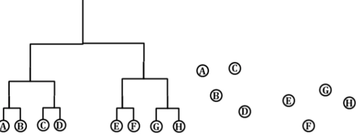
Figure 1 The left hand side of the graph representation is a cubic cladogram displayed with 8 sequences. The right hand side of the graph is the same 8 sequences visualized in 2D after dimension reduction.
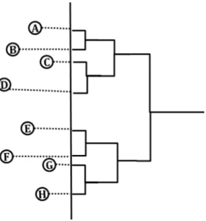
Figure 2 The example of choosing a random line to project all the sequences to and draw the given cubic cladogram accordingly.
Compared to the random choice shown in Figure 2, the projected tree is much clearer, and the correlations between the clustering result and the phylogenetic tree can be intuitively observed.
Figure 3 An example of a good choice of projection line as the dotted line within 8 sequences visualized in 2D space.
Figure 4 The example of choosing a good projection line determined by PCA to project all the sequences to and draw the given cubic cladogram accordingly.
because the phylogenetic tree displayed in the graph won’t show difference lengths between the leaf nodes and their parents. The phylogenetic tree here could be a rooted tree and an outgroup can be added as well. Once the plane with the largest variance is found for the 3D coordinates, the points are projected onto that plane. Then each pair of points, which correspond to each pair of leaf nodes shared the same parent are selected in the plane, their parent will be a new point which is the exact middle point of the connection between these two points. The parent will be draw one level higher than its children. The process is recursively done until all points, including the root and the outgroup points are drawn.
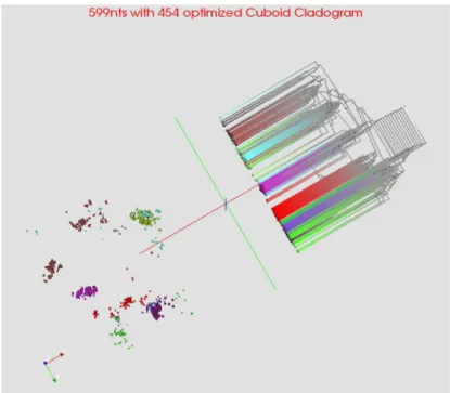
Figure 5 The screen shot from the side of the cuboid cladogram by choosing a plane using PCA on 599nts data using MSA and WDA-SMACOF
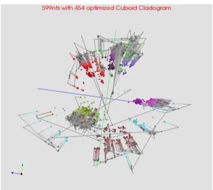
Figure 7 The screen shot from the top of the cuboid cladogram by choosing a plane using PCA on 599nts data using MSA and WDA-SMACOF
3. Spherical Phylogram
Figure 8 The example of distance calculation in a phylogenetic tree with 3 leaf nodes and 2 internal nodes.
The internal nodes cannot be directly observed because they represent hypothetical ancestor sequences, and therefore the distances from internal nodes to leaf nodes of the generated phylogenetic tree are unknown. By using RAxML, it is possible to calculate distance from an internal node to another node by using the summation over all the branches between them. For example, in Figure 8, the distance between point C and E can be calculated by summing over branch(C, B), branch(B, A) and branch(A, E). This distance calculation can generate a pairwise distance matrix for all the nodes based on all the branch lengths. However, the sum of branch lengths does not work to find the distance between pairs of leaf nodes since the pairwise distances between leaf nodes are already known from the MDS cluster visualization results. For example, the distance between leaf node C and D shown in Figure 5.5 is clearly not equal to branch(B, C) + branch(B, D). Therefore if the summation over the branches is used for defining distances during interpolation, the result will have a high bias because different distances were used for leaf nodes. But since leaf nodes already has coordinates in 3D, so this distance measurement maybe compared with the method in neighbor joining and do some future analysis.
[1]Ruan, Yang, Saliya Ekanayake, Mina Rho, Haixu Tang, Seung-Hee Bae, Judy Qiu, and Geoffrey Fox. "DACIDR: deterministic annealed clustering with interpolative dimension reduction using a large collection of 16S rRNA sequences." InProceedings of the ACM Conference on Bioinformatics, Computational Biology and Biomedicine, pp. 329-336. ACM, 2012.
[2] Ruan, Yang, Geoffrey House, Saliya Ekanayake, Ursel Schütte, James D. Bever, Haixu Tang, and Geoffrey Fox. "Integration of Clustering and Multidimensional Scaling to Determine Phylogenetic Trees as Spherical Phylograms Visualized in 3 Dimensions."Proceedings of C4Bio(2014): 26-29.