https://doi.org/10.5194/bg-16-831-2019
© Author(s) 2019. This work is distributed under the Creative Commons Attribution 4.0 License.
Towards a more complete quantification of the global carbon cycle
Miko U. F. Kirschbaum1, Guang Zeng2, Fabiano Ximenes3, Donna L. Giltrap1, and John R. Zeldis4
1Landcare Research – Manaaki Whenua, Private Bag 11052, Palmerston North 4442, New Zealand 2National Institute of Water & Atmospheric Research, Private Bag 14901, Wellington 6021, New Zealand 3Forest Science Unit, New South Wales Department of Primary Industries, Locked Bag 5123,
Parramatta, New South Wales 2150, Australia
4National Institute of Water & Atmospheric Research, PO Box 8602, Christchurch 8011, New Zealand
Correspondence:Miko U. F. Kirschbaum ([email protected]) Received: 3 October 2018 – Discussion started: 1 November 2018
Revised: 17 January 2019 – Accepted: 18 January 2019 – Published: 14 February 2019
Abstract. The main components of global carbon budget calculations are the emissions from burning fossil fuels, ce-ment production, and net land-use change, partly balanced by ocean CO2uptake and CO2 increase in the atmosphere.
The difference between these terms is referred to as the resid-ual sink, assumed to correspond to increasing carbon stor-age in the terrestrial biosphere through physiological plant responses to changing conditions (1Bphys). It is often used
to constrain carbon exchange in global earth-system models. More broadly, it guides expectations of autonomous changes in global carbon stocks in response to climatic changes, in-cluding increasing CO2, that may add to, or subtract from,
anthropogenic CO2emissions.
However, a budget with only these terms omits some im-portant additional fluxes that are needed to correctly infer
1Bphys. They are cement carbonation and fluxes into
in-creasing pools of plastic, bitumen, harvested-wood products, and landfill deposition after disposal of these products, and carbon fluxes to the oceans via wind erosion and non-CO2
fluxes of the intermediate breakdown products of methane and other volatile organic compounds. While the global bud-get includes river transport of dissolved inorganic carbon, it omits river transport of dissolved and particulate organic car-bon, and the deposition of carbon in inland water bodies.
Each one of these terms is relatively small, but together they can constitute important additional fluxes that would significantly reduce the size of the inferred 1Bphys. We
estimate here that inclusion of these fluxes would reduce
1Bphys from the currently reported 3.6 GtC yr−1 down to
about 2.1 GtC yr−1(excluding losses from land-use change). The implicit reduction in the size of 1Bphys has important
implications for the inferred magnitude of current-day bio-spheric net carbon uptake and the consequent potential of future biospheric feedbacks to amplify or negate net anthro-pogenic CO2emissions.
1 Introduction
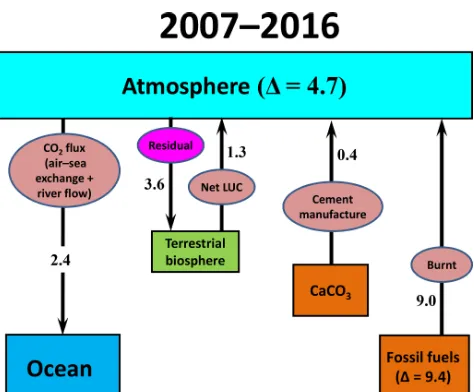
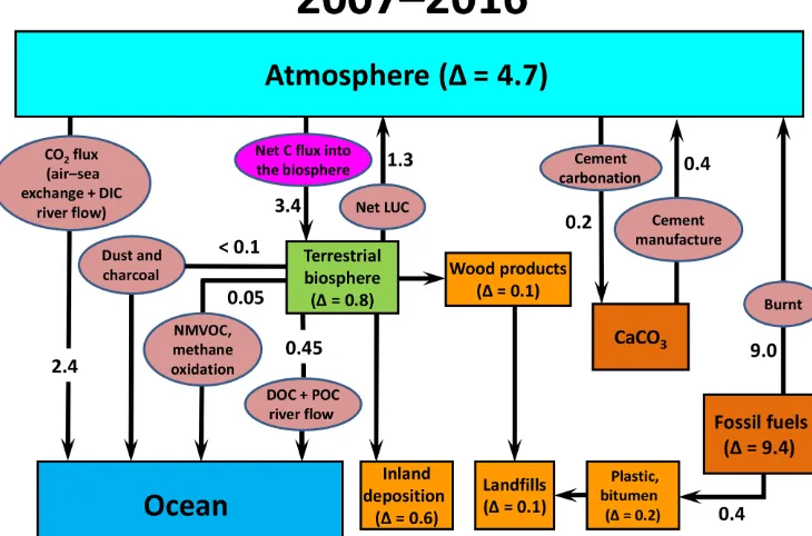
In its summarised form, the global carbon cycle is usu-ally expressed in the form of six main fluxes (Le Quéré et al., 2018; Fig. 1). Carbon is added to the atmosphere by the burning of fossil fuels (9.0 GtC yr−1), cement produc-tion (0.4 GtC yr−1), and ongoing deforestation, mainly in the tropics (1.3 GtC yr−1). Some fossil fuels (0.4 GtC yr−1) are also utilised for the manufacture of other products, like plas-tics, or are incompletely combusted and thus do not directly emit CO2to the atmosphere. The atmospheric CO2
concen-tration has increased to over 400 ppm through annual net ad-ditions of about 4.7 GtC yr−1, whereas the oceans overall are still close to their pre-industrial effective equilibrium con-centration of 280 ppm. This difference constitutes a driving force for ocean CO2 uptake, estimated at 2.4 GtC yr−1(Le
Quéré et al., 2018).
Figure 1. The main components of the global carbon cycle for the 2007–2016 period (after Le Quéré et al., 2018). Annually, 9.4 GtC yr−1of fossil fuels were used of which 0.4 GtC yr−1were not oxidised but used for manufacturing secondary products, like plastics, or incompletely combusted so that only 9.0 GtC yr−1were released to the atmosphere. The ocean flux consists of estimated air-ocean CO2exchange plus river flux of inorganic CO2.
The size of the residual sink is often implicitly or explic-itly equated with carbon uptake by the terrestrial biosphere (e.g. Ciais et al., 2013; Sitch et al., 2015; Arneth et al., 2017; Huntzinger et al., 2017). A sink of 3.6 GtC yr−1suggests that one-third of anthropogenic emissions might be balanced by biospheric carbon uptake and storage. The size of this flux is even more important for future trends in biospheric uptake that could provide an important positive or negative feedback for atmospheric CO2changes (Cramer et al., 2001; Jones et
al., 2013). If the magnitude of terrestrial uptake is over- or underestimated, it would lead to incorrect inference of the strength of future feedback processes between the terrestrial biosphere and the earth’s net carbon budget.
However, in the global carbon budget as presented in Fig. 1, several important fluxes have been omitted. In the present work, we aim to provide a quantification of these ad-ditional terms based on values found in the existing litera-ture or derived in the current work, and thereby more com-pletely quantify the global carbon cycle. In addition, we es-timate the actual increase in carbon stored in the terrestrial biosphere,1Bact, by explicitly accounting for the carbon flux
into additional carbon-storage pools or through pathways not previously included in global budget calculations. We also estimate the net change in carbon stored in the terrestrial biosphere, 1Bphys, to refer to the change in stored carbon
through physiological plant responses but excluding the ef-fects of land-use change (LUC).
Hence, the present work aims to quantify these additional terms:
1. Net increases in the pools of harvested-wood products, plastic, bitumen, rubber, leather, and textiles while they are in service;
2. Net increases of carbon in anaerobic landfills after sub-sequent disposal of these products;
3. The carbonation of previously manufactured cement products;
4. River transport from the land to the oceans as dissolved or particulate organic carbon (DOC or POC);
5. Carbon deposition in inland water bodies;
6. Transfer of carbon from the land to the oceans via aeo-lian transport either attached to mineral dust or as char-coal;
7. Fluxes of non-CO2 carbonaceous gases, principally
methane and NMVOCs (non-methane volatile organic compounds), and their intermediate breakdown prod-ucts.
Of these, CO2fluxes associated with cement carbonation (Xi
et al., 2016) and carbon deposition in fresh-water bodies (e.g. Regnier et al., 2013) constitute obvious fluxes from the atmo-sphere into relevant storage pools that have not previously been included in global budgets. There is also a sizeable net flux into the pool of harvested-wood products (Lauk et al., 2012). This flux has already been included in net land-use change calculations (Le Quéré et al., 2018), but in the in-terest of transparency it would be preferable if that flux was quantified more explicitly.
Net carbon fluxes into the pools of plastic and bitumen and subsequently into anaerobic landfills have also been in-cluded indirectly by accounting for only an assumed fraction of fossil-fuel carbon being oxidised (e.g. Marland and Rotty, 1984; Le Quéré et al., 2018). A small fraction of fossil fu-els is used for manufactured products, such as plastic and bitumen, and of the fossil fuels that are burnt, another small fraction is only incompletely combusted leading to less than 100 % being converted to CO2 (Marland and Rotty, 1984).
Based on these considerations, Marland and Rotty (1984) estimated oxidation fractions of 98 %, 91.8 %, and 98.2 % for the utilisation of gas, liquid, and solid fuels, respectively. These terms are then applied to fossil-fuel production data to derive fossil-fuel-based CO2 emission rates (e.g. Andres et
al., 2012). In the interests of greater transparency, it would be desirable, however, if fluxes through these key product pathways were more explicitly accounted for and reported in future global emission budgets.
Carbon transport to the oceans through river transport (Regnier et al., 2013), aeolian fluxes (e.g. Romankevich et al., 2009), or gas fluxes by carbonaceous compounds other than CO2all constitute additional carbon fluxes from the land
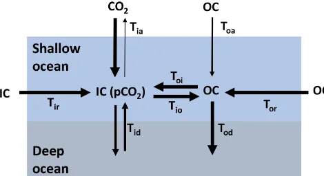
Figure 2.Illustration of the key carbon fluxes from the atmosphere to the deep oceans, with subscripts “i” and “o”; referring to inor-ganic and orinor-ganic forms of carbon, respectively.TiaandToaare
ex-changes with the atmosphere,TirandTorare river transport,Tioand Toiare the inter-conversions between organic and inorganic forms
in the ocean, andTidandTodare the transfers from shallow to deep
oceans.
for in the standard quantification of the global carbon cycle, and a more complete quantification is given below. The sig-nificance of the different terms in land–ocean exchange are discussed in the next section.
2 Ocean exchange
In deriving the global carbon budget, Le Quéré et al. (2018) used estimates of air–ocean CO2 exchange rates (Tia in
Fig. 2) and added the transport of inorganic carbon via river transport (Tir, Fig. 2) with the aim of describing the
anthro-pogenic carbon budget (Jacobson et al., 2007; Le Quéré et al., 2018). However, this omits other important transport path-ways as illustrated in Fig. 2. The ultimate key fluxes are the net transport of carbon from the shallow to the deep ocean (or to ocean-floor deposition in shallow seas) as either inorganic CO2(H2CO3, HCO−3, CO
2−
3 ), including solid CaCO3, or in
any soluble or particulate organic form. Hence, the relevant total carbon transfer,Tc, can be described asTc=Tid+Tod
whereTid andTod are the net carbon transfers to the deep
ocean of inorganic and organic carbon, respectively. The shallow ocean is too small for significant carbon storage, but the deep ocean has a large carbon-storage capacity. The shal-low ocean is important, however, as the interface between the ocean and the atmosphere and where pCO2measurements
are taken for the estimation of net CO2exchange between
the atmosphere and the shallow ocean.
In the ocean, organic and inorganic forms of carbon tinuously interchange. Inorganic carbon is fixed and con-verted into organic forms by photosynthetic organisms. As these organisms die or are eaten by larger organisms, carbon is respired in inorganic form. The sizes of these conversion fluxes are not important in the present context, as carbon can ultimately be transferred to depth in either organic or
inor-ganic form. The net flux of inorinor-ganic carbon from the deep ocean may even be negative, with net carbon transfer to depth reliant on organic carbon transfer.
As transfersTidandTod are difficult to measure directly,
the fluxTcis normally approximated asTc=Tia+Tirwhile
the fluxes of organic carbon from atmospheric transfer or river transport,ToaandTor, are ignored and omitted from the
estimated global fluxes. Instead, we propose that the more appropriate total flux should be calculated asTc=Tia+Tir+ Toa+Tor. Below, we quantify the different fluxes of organic
carbon to the oceans to complete the overall sums.
3 Calculation details
For comparison between the residual sink and estimates of carbon exchange of the land biosphere, we used the data given by Le Quéré et al. (2018) as land sink and budget imbalance for different years. Previous carbon budgets (e.g. Le Quéré et al., 2016) provided numbers denoted as residual sink activity. In the 2018 budget, this has been disaggregated into a land sink, estimated from biosphere models, and a bud-get imbalance term (Le Quéré et al., 2018). The sum of these two terms equates to the previously given residual sink,Sr.
Changes in terrestrial C stocks were calculated as
1Bphys=Sr−Rd−Rp−Ri−D−V−C−1P
−1B−1L+N (1)
1Bact=1Bphys+LUC, (2)
whereRd is river transport as DOC; Rp is river transport
as POC;Riis carbon deposition in inland waterways; Dis
carbon transport to the oceans as aeolian dust deposits;V
is transfer from volatile intermediate oxidation products of methane and NMVOCs;C is carbon storage in cement car-bonation;1P,1B, and1Lare the changes in carbon stored in plastics, bitumen, and landfills, respectively; andN is the non-oxidised fraction of fossil consumption that has been im-plicitly included in previous budgets. The terms1P,1B, and1Ltherefore largely cancel out the termN, but the cal-culations are made more explicit here.
The term1Bact refers to the actual change in total
ter-restrial biosphere carbon stocks, including changes due to land-use change, and 1Bphys refers to biospheric
carbon-stock changes due to physiological and age-class effects, but excluding land-use change. LUC is the carbon-stock change due to land-use change with negative numbers de-noting net losses to the atmosphere. Of these various com-ponents, no temporal trends were available forRd,Rp,Ri, D or V, but temporal patterns could be included for 1P,
1B,C,1L, andNbased on the work of Lauk et al. (2012) and Xi et al. (2016) and calculated, following Marland and Rotty (1984), as
whereFis total fossil-fuel consumption andg,landsare the percentages of gas, liquid, and solid fuel, respectively, in the global mix of fossil fuels, estimated as constant percentages of 17.0 %, 41.8 %, and 41.2 %, respectively; the constants in Eq. (3) have been taken from Marland and Rotty (1984).
4 Wood products, plastics, bitumen, and cement carbonation
For harvested-wood products, plastic, and bitumen in ser-vice by human societies, the relevant quantity in the present context is the net increase in the size of these pools. At the end of their service lives, plastic and harvested-wood prod-ucts, especially paper prodprod-ucts, may be reused, recycled, or disposed of either by incineration or disposal in landfills. If they are incinerated in waste-to-energy facilities, CO2is
re-leased to the atmosphere immediately, and if they are reused or recycled, the products re-enter the “in-service” pool. Al-ternatively, these products may be deposited in landfills in countries that use landfills as part of their waste management strategies, which will be discussed in the next section.
For harvested-wood products in service, net increases in carbon stocks primarily correspond to the pool of long-lived structural wood products, such as housing frames. Paper products, on the other hand, tend to have short service lives and do not build up to sizeable pools even though fluxes through these pools can be substantial. This can include mul-tiple passes through the active-service pool because paper products may be recycled repeatedly before eventual dis-posal. Le Quéré et al. (2018) included a simple term in the calculations of net land-use change that accounted for harvested-wood products. They assumed that a fraction of the wood lost through land-use change was not directly lost as CO2 to the atmosphere but retained in harvested-wood
products. However, we believe that a more explicit represen-tation of this pool, as provided through the work of Winjum et al. (1998) and Lauk et al. (2012), would be desirable for greater transparency.
The socio-economic models of Kayo et al. (2015) and Brunet-Navarro et al. (2016) have shown that in poorer soci-eties, wood use per person increases with increasing wealth (quantified as gross domestic product, GDP, per capita, cp−1). However, that relationship saturates at intermediate values of GDP cp−1 and even becomes negative for the wealthiest societies. Lauk et al. (2012) estimated that humans own on average approximately 1 tC cp−1of harvested-wood
products. If that value is remaining constant over time, one could assume an annual increase in the global pool by about 80 MtC yr−1 purely driven by global population growth. If wood use per person is also increasing, as shown by Kayo et al. (2015), it would result in an increase in the global harvested-wood-products pool by more than 80 MtC yr−1. Winjum et al. (1998) and Lauk et al. (2012) estimated changes in the harvested-wood-products pool from
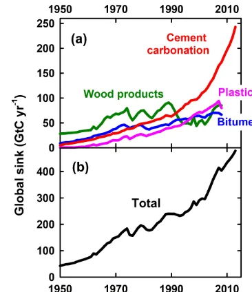
analy-Figure 3.Estimated net fluxes of carbon into the pools of harvested-wood products, plastics, bitumen, and cement carbonation since 1950(a)and their combined total(b). Based on data given in Lauk et al. (2012) and Xi et al. (2016).
sis of wood-production statistics and assumption of product longevities. Winjum et al. (1998) estimated an annual in-crease of about 140 MtC yr−1, while Lauk et al. (2012) pro-vided a slightly smaller estimate of recent increases of just under 100 MtC yr−1. Lauk et al. (2012) also provided histor-ical estimates over the 20th century (Fig. 3a).
However, for most countries and wood-product categories (paper, wood panels, and sawn wood), there are no reliable service life factors. Global analyses, therefore, have had to rely on the use of generic factors, such as IPCC default Tier 2 half-lives (IPCC, 2014). Lauk et al. (2012) considered the need to use these generic factors as the primary cause of the large uncertainties in their estimated carbon fluxes into harvested-wood-product pools. Lauk et al. (2012) also esti-mated fluxes into the pools of bitumen, used mainly for road construction, and plastics (Fig. 3a). Fluxes started from very low values before 1950 but have increased steadily and are now similar to fluxes into the pool of harvested-wood prod-ucts.
In the case of cement carbonation, the flux is associated with the degeneration of previously manufactured cement. Cement manufacture is essentially the calcination of CaCO3
into CaO under high temperature. The resultant CO2release
is included in global carbon budgets (Andrew, 2018) and ac-counts for about 4 % of total anthropogenic CO2emissions
(Le Quéré et al., 2018; Fig. 1). When cement is subsequently exposed to rain and natural CO2concentrations, the process
is reversed, and CO2is reabsorbed, replacing oxygen bound
[image:4.612.335.518.64.276.2]All cement is subject to that kind of degradation, with its rate decreasing with the thickness of the cement layer. Thinner layers of mortar therefore degrade faster than more solid concrete structures. When a building is demolished, ce-ment carbonation tends to increase as cece-ment becomes frag-mented, thereby opening new surfaces that assist the diffu-sional penetration of CO2. The rate of cement carbonation
can, therefore, be approximated as being proportional to total cumulative past cement production. Hence, global carbona-tion rates were likely to have been low in the 1950s, then increased gradually to the 1990s (Fig. 3a), with much more substantial increases since then. Using statistics of historical cement production in different categories, Xi et al. (2016) estimated recent uptake rates through carbonation of about 250 MtC yr−1, with uptake rates expected to continue in-creasing into the future.
The combined flux from these four fluxes (cement car-bonation and increasing pools of harvested-wood prod-ucts, plastic, and bitumen) was estimated to have been less than 50 MtC yr−1 in 1950 but increased steadily to about 300 MtC yr−1 by the year 2000 (Fig. 3b). The rate of up-take has increased more sharply since then, driven mainly by increasing cement carbonation, and is estimated to have reached about 450 MtC yr−1by 2010 (Fig. 3b).
5 Landfill storage
At the end of their service lives, products may be disposed of in landfills, where conditions may be aerobic, semi-aerobic or anaerobic depending on their management (IPCC, 2006). If materials are kept under anaerobic conditions, their effec-tive storage life can be extended substantially, with very slow decomposition and resultant carbon loss (Wang et al., 2011, 2015; Ximenes et al., 2015, 2018, 2019).
Wood and plastics are particularly persistent after disposal unless they are incinerated. Bitumen is not usually disposed of, but, when roads are renewed, old bitumen is typically recycled, with only minor losses (Lauk et al., 2012). Tex-tiles, rubber, and leather make additional minor contributions to total landfill carbon stocks. With all categories added to-gether, anaerobic landfills can thus store large amounts of carbon.
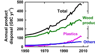
Lauk et al. (2012) estimated total annual disposal rates of various key products (Fig. 4), estimated at nearly 500 MtC yr−1. While Fig. 4 clearly shows the historical pat-tern of product disposal, it does not indicate what quanti-ties of products are disposed of in anaerobic landfills. To the best of our knowledge, there have been no prior estimates of global net carbon stock changes in landfills. We have there-fore attempted to provide a first global estimate of waste dis-posal in anaerobic landfills and consequent annual changes in landfill carbon stocks (Table 1).
[image:5.612.335.517.66.168.2]Accounting for annual landfill fluxes of different waste streams, their dry-matter percentages, carbon contents, and
Figure 4.Annual rates of disposal of harvested-wood products, plastics and other carbon containing compounds. Based on data given in Lauk et al. (2012).
relative permanence under anaerobic conditions, we esti-mated changes in long-term carbon pools in landfills for dif-ferent product categories. The temporal pattern of breakdown in landfills is not clear. One normally describes the break-down of products as an exponential decay process which can be described with simple decay constants or their in-verse, the residence times. However, under anaerobic condi-tions, breakdown effectively ceases completely, and a perma-nence factor essentially separates products into a fraction that breaks down over a relatively short time frame and a second fraction that does not break down at all within a time frame relevant for carbon management. The sizes of these fractions are determined by their associated degradability, such as cel-lulose to lignin ratios, and the biophysical conditions within landfill sites (e.g. Barlaz, 2006).
Paper and paperboard constituted the largest disposal cat-egory, but because of its relatively fast rate of degradation (Wang et al., 2011, 2015; Ximenes et al., 2015, 2018), its contribution to increasing carbon stocks is only minor. Al-though less wood and engineered-wood products (e.g. ply-wood, particle board) are disposed of in landfills than of pa-per and papa-perboard, it leads to a higher estimated storage flux because wood is highly resistant to degradation under anaerobic conditions (Ximenes et al., 2019). Plastics have the highest estimated storage flux (42 MtC yr−1) because of
their high disposal rate, high carbon content, and very high persistence.
Using the detailed data and assumptions in Table 1, we calculated a net change in landfill storage of 88 MtC yr−1.
6 River transport
Table 1.Waste generation and estimated disposal in anaerobic landfills.
Product Estimated total amount of material Dry Carbon Carbon in long- Estimated
disposed of in anaerobic matter fraction term storage storage flux landfills (Mt yr−1) (%) (%) (%) (MtC yr−1)
Wood and engineered-wood products 67 89 48 98 28
Paper and paperboard 80 94 39 44 13
Plastic 57 100 75 95 41
Textile and rubber 32 82 55 40 6
Total 236 88
“Carbon in long-term storage” refers to the estimated proportion of waste stored permanently in anaerobic landfill sites. Total disposal estimates were derived from various sources including countries’ greenhouse gas inventories for the Waste Sector, population statistics, IPCC documents (IPCC 2006, 2014), the European Atlas of Raw Materials (Prognos, 2008) and the World Bank Waste Reports (e.g. Hoornweg and Bhada-Tata, 2012). Moisture contents were obtained from Wang et al. (2015) and Ximenes et al. (2018). Carbon fractions were taken from the IPCC Good Practice Guidance (2014), and carbon-storage factors from Wang et al. (2011, 2015) and Ximenes et al. (2018). The dry matter and carbon fractions of the wood, engineered-wood products, and paper or paperboard were expressed as averages weighted by global market share of the various product categories (FAO, 2016). The estimates provided here are based on the most recent available information but were themselves based on older information largely covering the period since 2000. The numbers in bold in the bottom row have been used as our estimate of the contribution to global carbon fluxes.
Net fluxes into and out of inland water systems also consist of multiple entry points and large outgassing as some organic materials are broken down and respired as CO2before they
can be deposited in lake sediments or the oceans, while si-multaneously, some new carbon is fixed through aquatic pho-tosynthesis.
Mendonca et al. (2017) documented the largest reported emission rates per unit area for small reservoirs, with vari-ability that extended over 3 orders of magnitude, yet global estimates had to be based on a mere 59 available point esti-mates. The combined surface area of these smaller reservoirs is fortunately much smaller than that of large lakes which reduce the importance of that uncertainty. Larger lakes had similar relative variabilities in observed rates but smaller av-erages. However, the small number of available observations clearly prevents the size of this globally important flux to be estimated with high confidence (e.g. Regnier et al., 2013).
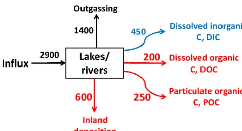
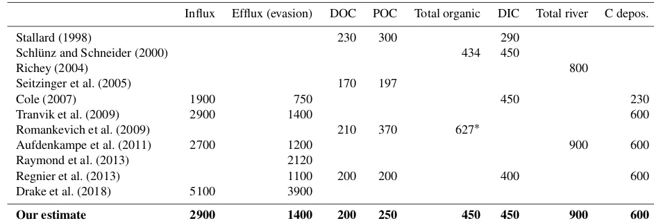
Despite these difficulties, various authors have attempted to provide global estimates of the key fluxes (Table 2; Fig. 5). Most authors have estimated total influx to inland water-ways of between 2700 and 2900 MtC yr−1, while the recent work by Drake et al. (2018) gave a much larger estimate of 5100 MtC yr−1 (Table 2). Of that amount of carbon enter-ing inland waterways, different authors have estimated out-gassing losses between 750 and 2120 MtC yr−1, with the es-timate of Drake et al. (2018) again being much larger at 3900 MtC yr−1. If one uses these estimates, together with some extra inputs from mineral weathering, this leaves about 1500 MtC yr−1 to be either deposited in inland water bod-ies or transported to the oceans (Table 2). Apart from the older work of Cole et al. (2007), most other authors esti-mated total inland deposition as 600 MtC yr−1and total flux to the ocean as 900 MtC yr−1, broken down into a DIC flux of 450 MtC yr−1, POC flux of about 250 MtC yr−1, and DOC
flux of 200 MtC yr−1. Romankevich et al. (2009) estimated
an additional contribution of 47 MtC yr−1from coastal ero-sion, ground-water influx, and glacial run-off.
Figure 5.The main carbon fluxes in MtC yr−1involving inland wa-terways. The number shown in blue is already included in the global carbon budget, whereas the numbers in red should be added to the revised global carbon budget. The numbers in black do not need to be included explicitly.
Considering the evidence used by the various authors, we consider total carbon flux to inland waterways to most likely be about 2900 MtC yr−1 (Fig. 5; Table 2). About half of that (1400 MtC yr−1) is lost from waterways by outgassing, although neither of those estimates are needed for explicit inclusion in the global budget. The important flux is the transport to the oceans, consisting of 450 MtC yr−1 DIC, 200 MtC yr−1DOC, and 250 MtC yr−1 POC (Table 2). The DIC flux is already included in the estimate of total inor-ganic ocean uptake, but the DOC and POC fluxes have not been included in the global summary numbers of Le Quéré et al. (2018). In addition, between 60 and 250 MtC yr−1are
[image:6.612.312.548.276.404.2]Table 2.Summary of prior estimates of the main components of carbon fluxes through inland waterways.
Influx Efflux (evasion) DOC POC Total organic DIC Total river C depos.
Stallard (1998) 230 300 290
Schlünz and Schneider (2000) 434 450
Richey (2004) 800
Seitzinger et al. (2005) 170 197
Cole (2007) 1900 750 450 230
Tranvik et al. (2009) 2900 1400 600
Romankevich et al. (2009) 210 370 627∗
Aufdenkampe et al. (2011) 2700 1200 900 600
Raymond et al. (2013) 2120
Regnier et al. (2013) 1100 200 200 400 600
Drake et al. (2018) 5100 3900
Our estimate 2900 1400 200 250 450 450 900 600
∗For the total organic C flux to the ocean, in addition to DOC and POC fluxes, Romankevich et al. (2009) also estimated fluxes of 25 MtC yr−1from coastal erosion, 14 MtC yr−1from ground-water influx, and 8 MtC yr−1from glacial run-off. The numbers in bold in the bottom row have been used as our estimate of the contribution to global carbon fluxes.
7 Aeolian fluxes
Carbon can also be transported from the land to the oceans by aeolian transport through wind erosion of dust particles (Zender et al., 2003; Webb et al., 2012). These carbon fluxes to the ocean are not captured in air–sea CO2 exchange but
add to the total flux of carbon from the land to the ocean (see Fig. 2).
Romankevich (1984) estimated aeolian carbon flux as 320 MtC yr−1, while Romankevich et al. (2009) estimated it as 96 MtC yr−1. Estimates can also be based on indepen-dently estimating the annual flux of aeolian dust and its car-bon concentrations. Mahowald et al. (2005) summarised the different available estimates of the total aeolian dust flux as 1500–2000 Mt(dust) yr−1. Assuming source carbon concen-trations between 1 % and 2 % (Webb et al., 2012; Chappell et al., 2013) and a 2.5-fold enrichment of carbon concentrations in dust relative to source concentrations (Webb et al., 2005), it leads to a global flux estimate of 50–100 MtC yr−1.
8 Charcoal
A sizable fraction of annually produced biomass is burnt each year (Kuhlbusch and Crutzen, 1995). Savannah vegetation is particularly prone to annual burning, and a fraction of burnt material is not combusted completely but remains as char-coal, estimated as 50–270 MtC yr−1(Forbes et al., 2006). A small fraction of that will become airborne, either during fires themselves or in subsequent wind storms, and a small pro-portion of that airborne fraction will be transported to the oceans. Forbes et al. (2006) estimated this flux to be less than 10 MtC yr−1.
9 Methane and NMVOCs
The principal gas transfer of carbon to the oceans is via CO2,
but carbon can also reach the ocean in organic gaseous form (Fowler et al., 2009). The annual combined flux of methane and NMVOCs is estimated to be about 1.3 GtC yr−1, with methane fluxes contributing about 500 MtC yr−1 (Ciais et al., 2013; Kirschke et al., 2013) and NMVOCs about 800 MtC yr−1 (Fowler et al., 2009), more than half of which is isoprene. Most of these compounds are oxidised in the troposphere, with methanol, methyl hydroperoxide, and formaldehyde as key intermediate oxidation products (Fig. 6). If these compounds were fully oxidised to CO2in
the atmosphere, there would be a simple closed loop between production by the terrestrial biosphere and atmospheric ox-idation, but any transfer to the ocean by compounds other than CO2constitutes an additional carbon transfer from land
to the ocean (see Fig. 2) that is not otherwise captured in the budget.
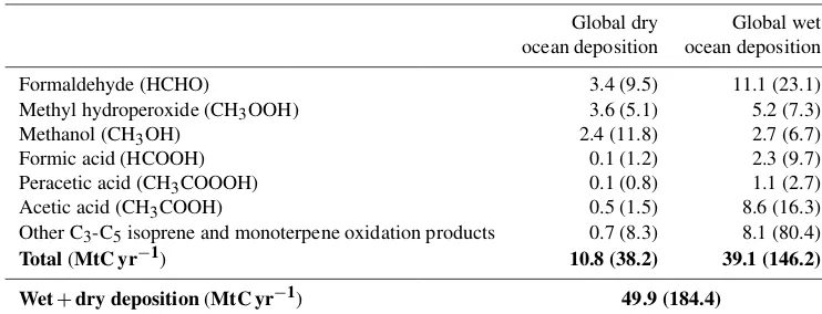
This transfer can be by direct transfer to the surface ocean or after prior solution in raindrops. This direct flux of methane and isoprene is probably small due to their low wa-ter solubility. However, under partial oxidation in the atmo-sphere, major intermediate products are methanol, organic acids, and formaldehyde, which are all highly soluble in wa-ter and can be deposited in the oceans as wet (afwa-ter dissolu-tion in rain or fog) or “dry” deposidissolu-tion when gases dissolve directly in ocean water. As we are not aware of prior esti-mates of this flux, we have estimated wet and dry deposi-tion of the relevant compounds here, including a separadeposi-tion between land and ocean deposition (Table 3). Details of the calculation methods are given in the Supplement.
deposi-Table 3.Estimated annual carbon fluxes to the world’s oceans and globally (values in brackets) from dry and wet deposition of VOCs and their oxidation products. Data have been calculated with the NIWA-UKCA CCM model. Units are in MtC yr−1. The numbers in bold in the bottom rows have been used as our estimate of the contribution to global carbon fluxes.
Global dry Global wet ocean deposition ocean deposition
Formaldehyde (HCHO) 3.4 (9.5) 11.1 (23.1)
Methyl hydroperoxide (CH3OOH) 3.6 (5.1) 5.2 (7.3)
Methanol (CH3OH) 2.4 (11.8) 2.7 (6.7)
Formic acid (HCOOH) 0.1 (1.2) 2.3 (9.7)
Peracetic acid (CH3COOOH) 0.1 (0.8) 1.1 (2.7)
Acetic acid (CH3COOH) 0.5 (1.5) 8.6 (16.3)
Other C3-C5isoprene and monoterpene oxidation products 0.7 (8.3) 8.1 (80.4)
[image:8.612.112.483.107.249.2]Total(MtC yr−1) 10.8 (38.2) 39.1 (146.2) Wet+dry deposition(MtC yr−1) 49.9 (184.4)
Figure 6.The main fluxes involved in the transfers of methane and NMVOCs to the oceans. Details of the estimated fluxes are given in Table 3.
tion of 10.8 MtC yr−1and wet deposition of 39.1 MtC yr−1, which together account for around 27 % of total surface de-position (with 73 % assumed to occur over land). Some of these intermediate products have short lifetimes and are, therefore, mainly deposited close to their points of produc-tion, which are mostly over land areas.
Summing these various fluxes provides an additional
∼50 MtC yr−1of non-CO2flux from the atmosphere to the
oceans. Any estimate of global fluxes depends strongly on deposition schemes, chemical mechanisms, and terrestrial NMVOC emissions, which vary among global models and are poorly constrained by observations. Hence, there are con-siderable uncertainties in these estimated fluxes, as demon-strated by Jacob et al. (2005), for example, in the case of the global methanol budget. They summarised the results of various previous studies and reported global dry depo-sition on the oceans estimated by different models of 0.3–
50 Mt(CH3OH) yr−1 plus total global wet deposition of 9–
50 Mt(CH3OH) yr−1which was not separated between land
and ocean deposition.
This illustrates the remaining levels of uncertainties in these global estimates. There are also considerable differ-ences in isoprene and monoterpene oxidation mechanisms among the models, in particular the formation of interme-diate products from isoprene oxidation (e.g. Paulot et al., 2009). Some further information on these uncertainties is given in the Supplement.
10 Summary of the main fluxes in the global carbon cycle
Consideration of these additional pools and fluxes reduces the estimated additional carbon stored in the terrestrial bio-sphere,1Bphys, from 3.6 to 2.1 GtC yr−1 (Fig. 7, Table 4).
While none of the various extra fluxes are particularly large or important on their own, added together they reduce the size of the inferred terrestrial biosphere sink by about 1.5 GtC yr−1.
For greater transparency, it would also be desirable to ex-plicitly include harvested-wood products and landfill pools. The associated carbon flux is already included under the net-land-use calculations (Le Quéré et al., 2018). Inclusion of a harvested-wood-products pool, therefore, would not affect the size of the residual sink, but it would require a corre-sponding adjustment of the net land-use-change flux.
[image:8.612.77.261.147.444.2]in-Figure 7.Expanded summary of the main components of the global carbon cycle for the 2007–2016 period. The fluxes are those given by Le Quéré et al. (2018) as shown in Fig. 1 above. These broad fluxes have then been modified based on Table 4 and the details provided in specific sections above. Rectangular boxes refer to identified important carbon storage pools in the global carbon budget. Fluxes described in ovals refer to key fluxes between these storage pools.
Table 4.Adjustments to the estimated change in the terrestrial bio-sphere (GtC yr−1). The term1Bactrefers to all actual biospheric
carbon-stock changes, including those due to LUC whereas1Bphys excludes LUC effects and includes only physiological and age-class effects. The “inferred flux into the biosphere” is calculated as the residual sink minus cement carbonation.
Original residual uptake 3.6
Cement carbonation −0.2
Revised inferred flux into the biosphere 3.4
inland deposition −0.6
river transport (DOC, POC) −0.45 Flux of methane, NMVOC+intermediates −0.05
Aeolian dust transport −0.05
Harvested-wood-products pool −0.1
Change in landfill pool originating −0.05 from harvested-wood products
LUC −1.3
1Bact 0.8
1Bphys 2.1
creasing landfill carbon storage is less well constrained, as we could find no prior global assessment of this flux. We have provided the first such global estimate in the present work, but significant uncertainty remains due to incomplete knowledge of regional details of the key properties of
differ-ent waste streams. In any case, explicit inclusion of fluxes into these storage pools would be desirable to increase trans-parency of the overall global carbon budget.
These incomplete oxidation terms for fossil-fuel use (Mar-land and Rotty, 1984) account for incomplete combustion during energy generation and for non-fuel uses. That has been represented explicitly in Fig. 7. For internal consis-tency, the fossil-fuel consumption rates have therefore been increased by 0.4 GtC yr−1so that non-fuel uses are given ex-plicitly in Fig. 7. While, for transparency, it would be de-sirable to make these fluxes explicit, it would not affect the estimated size of the residual sink.
Cement carbonation is an additional sink that is likely to increase in proportion to the cumulative total amount of man-ufactured cement and is, therefore, likely to increase further into the future. Its magnitude is also reasonably well con-strained and is clearly bounded by the total historical cement production. This flux has so far been omitted from the global carbon budget, and its inclusion reduces the size of the resid-ual sink.
[image:9.612.118.483.76.317.2]vari-ous global estimates are converging on similar flux estimates (e.g. Regnier et al., 2013; Drake et al., 2018).
A fraction of this organic carbon flux is oxidised in the shallow ocean, leading to outgassing in some regions (e.g. Borges et al., 2005; Jacobson et al., 2007). Another fraction is transferred to the ocean floor or the deep ocean in organic form. POC associated with soil minerals is particularly prone to direct sinking to the ocean floor. That mineral-associated fraction should obviously be included. The fraction that is oxidised in the shallow ocean and converted to inorganic car-bon will increase the surfacepCO2(partial pressure of CO2).
This lowers the atmosphere-to-ocean CO2 gradient and
re-duces ocean CO2uptake, or can even lead to outgassing.
Cal-culations of ocean CO2 uptake by gaseous exchange could
be correctly estimated without bias, but total transfer of CO2
to the surface ocean will be the combined flux of air–sea ex-change plus the additional contribution of organic carbon that found its way to the ocean by aeolian or river transfer, or by gas transfer of non-CO2 carbon compounds. Regardless of
those further transformations, Fig. 2 showed that it would be appropriate to include this flux of organic carbon as an im-portant addition to the overall budget.
Deposition of carbon in inland waterways is another quan-titatively important flux into an additional carbon storage pool that should be included in the overall budget. With the increasing regulation of waterways and the construction of more dams on the world’s rivers (e.g. Regnier et al., 2013), and possible increases in erosion fluxes (e.g. Yang et al., 2003), this flux is also likely to continue to increase into the future.
Some of the erosion-related components of this flux con-stitute a simple lateral carbon transfer from erosion sites to some downstream waterways with no net effect on the atmo-sphere. However, most denuded erosion sites can eventually regain their lost soil organic carbon. While that process is slow and may remain incomplete, the resultant potential car-bon gain needs to also be factored in (van Oost et al., 2007). It would, therefore, be too simplistic to ignore inland deposi-tion as just a lateral transfer. In its totality, erosion may act as a net sink or source of carbon to the atmosphere. For global carbon accounting purposes, it means that inland deposition should be included, but any changes in soil carbon stocks also need to be quantified to complete the overall balance.
The next relevant flux is the transport of carbon attached to aeolian dust or charcoal. Again, this flux transfers car-bon from the land surface to the oceans through means that are not quantified through CO2 exchange at the
[image:10.612.304.550.67.163.2]air-surface interchange. This flux may contribute an additional 50–100 MtC yr−1. Finally, methane, NMVOCs, and their in-termediate oxidation products can be transferred directly to the oceans. As with river and aeolian transport, the subse-quent fate of these products after they reach the oceans does not change their important role as a carbon-transfer mech-anism, and therefore these fluxes should be included. Here,
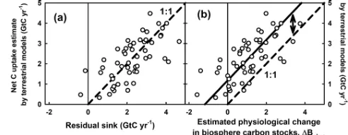
Figure 8.Mean estimates of net carbon uptake by the biosphere plotted against the residual sink(a), or as a function of the revised 1Bphyscalculated here(b). Data have been taken from Le Quéré
et al. (2018), with each point corresponding to an annual flux es-timate since 1959. Data were calculated as given in Eq. (1). The dashed lines are 1:1 lines, and the solid line in(b)is off-set by 1.2 GtC yr−1but retains a slope of 1.
we have provided a first global estimate of the size of these combined fluxes of about 50 MtC yr−1.
The sizes of these various fluxes have been estimated in previous publications that have focused on one process or an-other, or they have been calculated based on existing under-lying information where no prior global estimates could be found. The novel contribution of the present analysis is bring-ing these fluxes together in a combined assessment (Fig. 7), which has not previously been done. While the exact mag-nitude of some of these fluxes remains uncertain, it is clear that they are not zero. Their exclusion from past global car-bon budgets has, therefore, systematically inflated the size of the estimated1Bphys. It is, therefore, warranted to include
them in future budgets and move towards a better, and less biased, estimate of1Bphys and the residual sink strength of
the terrestrial biosphere.
11 Implications for biosphere models
The residual sink is often implicitly or explicitly equated with net exchange by the biosphere, with the two flux estimates even presented on the same graph by Ciais et al. (2013), and Le Quéré et al. (2018) referred to the residual sink as the “land sink”. The size of the residual sink has thus been used as an important reality check of the structure and parameterisation of existing biosphere models.
However, equating the residual sink to1Bphyswithout
ac-counting for these additional fluxes has led to an overestima-tion of1Bphys with important implications for our
assess-ment of the veracity of existing biosphere models (Fig. 8). Taking the annual flux estimates generated by the average of accepted biosphere models and the size of the originally calculated residual sink, one obtains a fairly good relation-ship, with estimates largely conforming to a 1 : 1 relationship (Fig. 8a).
against the 1:1 line is poor. There is a large discrepancy with the biosphere models estimating sink activity that is about 1.0–1.5 GtC yr−1higher than the corresponding estimates of
the revised residual sink activity (Fig. 8b). This suggests that current biosphere models systematically overestimate bio-spheric carbon uptake, which has important implications for present-day overall global carbon fluxes. It suggests that bio-sphere models may similarly overpredict future carbon up-take rates. If enhanced carbon upup-take by the terrestrial bio-sphere in response to climate change, including increasing atmospheric CO2, is overestimated, it will similarly
overesti-mate the extent by which biospheric feedbacks could negate future anthropogenic greenhouse gas emissions.
12 General discussion
An understanding of the global carbon cycle is important for a full appreciation of the anthropogenic disturbance of the cycle, and to what extent that disturbance is negated, or amplified, through natural feedback processes. It is even more important as a guide to the magnitude of future feed-back processes (e.g. Cramer et al., 2001; Friedlingstein et al., 2006; Jones et al., 2013; Huntzinger et al., 2017). It is important to anticipate whether any current carbon uptake by the biosphere may be reversed under future climatic con-ditions, especially under ongoing and intensifying warming (e.g. Kirschbaum, 2000), while plants may become less re-sponsive to CO2as atmospheric concentrations trend towards
CO2saturation (e.g. Friedlingstein et al., 2006).
The comparisons between the residual sink and biospheric net CO2uptake have been given explicitly by the IPCC (Ciais
et al., 2013), and they play an important role as a reality check of global biosphere models (e.g. Arneth et al., 2017; Huntzinger et al., 2017). However, to fulfil that role, it is es-sential that the comparisons use comparable data. It is there-fore important to calculate 1Bphys after the various known
terms listed above have been explicitly quantified and sub-tracted from the “residual sink”.
To correctly anticipate whether future natural biospheric carbon exchange will add to or subtract from anthropogenic emissions, it is essential to assign sink activity to the appro-priate processes. If sink activity is assumed to relate to net uptake by the biosphere, one might expect it to respond to factors such as the age class distribution of forests, or tem-perature, precipitation, CO2concentration, or land
manage-ment. If one incorrectly infers the sensitivity of the system to these external factors, it would be impossible to predict future biospheric responses.
The various factors identified above respond to different drivers. Aeolian fluxes, for example, might respond to cli-mate variability like the ENSO cycle and longer-term land-use and management choices, and fluxes related to the oxi-dation of methane and NMVOCs would be proportional to the underlying fluxes of methane and NMVOCs. Storage in
increasing pools of plastic, bitumen, and landfills, as well as cement carbonation, are clearly determined by anthropogenic factors, such as economic and technological development. Future fluxes, therefore, will not respond to future temper-ature or CO2concentration, but need to be assessed through
assessment of socio-economic developments.
Terrestrial net carbon exchange can be further subdivided into at least four distinct processes,
12.1 Growth rate changes related to forest age
Forest growth tends to be highest in young stands and de-creases as stands age (Ryan et al., 1997; Kurz and Apps, 1999). Any net forest growth can therefore be due to the rebound of forest biomass after prior disturbance through anthropogenic or natural processes. Disturbance may be through the harvesting of established forests or the planting of new ones, or due to natural factors, such as wildfire or insect-pest outbreaks (e.g. Stinson et al., 2011). The presence of a global net forest sink implies that new growth exceeds losses through wood extraction and other disturbance fac-tors. A forest sink can be caused by disturbance-related car-bon losses in preceding years. Understanding forest growth under current and future conditions therefore requires dis-turbance effects and age-class distributions to be combined with an assessment of biophysical growth factors (e.g. Chen et al., 2000). Many of the world’s forests are now being in-ventoried at regular intervals (Pan et al., 2011), which can be supplemented with remotely sensed information (Dong et al., 2003). Growth responses can be inferred from these changes in age-class distribution (Stinson et al., 2011), although sub-tler disturbance-related effects on woody biomass are diffi-cult to fully capture at the global scale and may have led to past underestimation of carbon emissions related to land-use change (Arneth et al., 2017), with a consequent larger rebound potential as well.
12.2 Growth rate changes related to biophysical drivers
In principle, growth can be enhanced by increasing CO2
con-centrations (Pugh et al., 2016; Hickler et al., 2015), nitrogen deposition from industrial pollution (LeBauer and Treseder, 2008), or climatic changes apart from increasing CO2
nutri-ent availability can retain an over-riding importance for stand productivity.
12.3 Blue carbon
It has been recognised that mangrove forests, seagrass beds, and salt marshes can sequester large amounts of carbon, re-cently termed “blue carbon” (McLeod et al., 2011; Huxham et al., 2018). It has been estimated to constitute a global car-bon sink of at least 200 MtC yr−1(McLeod et al., 2011) or even more (Breithaupt et al., 2012). However, infrastructure development of coastal habitats not only prevents ongoing carbon sequestration by these ecosystems but can also lead to the release of the large carbon stocks of these systems. Overall, such development may result in comparable annual carbon losses as the ongoing sequestration by intact systems (e.g. Pendleton et al., 2012; Regnier et al., 2013; Atwood et al., 2017).
12.4 Soil organic carbon
There may also be changes in soil carbon that can be very dif-ficult to detect. Globally, there are about 2500 GtC in soil or-ganic matter to a depth of 2 m (Batjes, 2004) so that a change by just 0.4 % yr−1would equate to a flux of 10 GtC yr−1to or from the atmosphere (Minasny et al., 2017). Such a change could be readily associated with land-use changes (e.g. Guo and Gifford, 2002; Kim and Kirschbaum, 2015). They may also correspond to episodic changes within given land uses, especially changes related to accelerated erosion under agri-cultural land use (e.g. van Oost et al., 2007; Quinton et al., 2010; de Rose, 2013).
Observational verification of annual changes of the order of 0.4 % yr−1is extremely difficult owing to the many im-portant factors that may positively or negatively affect soil carbon levels under different circumstances and over differ-ent timescales (e.g. Schipper et al., 2017). However, even such proportionately small changes could be very important in the global budget and have become the basis of the recent
4 per milleinitiative (e.g. Minasny et al., 2017) which aims to promote land-use practices to increase soil carbon by that amount.
13 Conclusions
It is important to ensure that anthropogenic CO2emissions
do not lead to changes in atmospheric CO2 concentrations
with dangerous consequences for nature and society. A good understanding of the global carbon budget is essential for a good assessment of current and likely future trends in car-bon stocks and fluxes. However, the global carcar-bon budget in its currently used form is overly simplified and, there-fore, does not provide appropriate guidance on the way an-thropogenic and natural processes interact to lead to the ob-served increases in atmospheric concentrations. It also does
not provide sufficient detail on some important component fluxes, which hinders a full appreciation of their role in the global budget. These simplifications warrant modifications to the budget to explicitly and comprehensively include other known carbon fluxes between major carbon pools. While the magnitude of these various fluxes remains uncertain, under-standing of the key processes has grown over the years so that it has become appropriate for these additional fluxes to be explicitly included in future global budgets.
The greatest practical importance of that inclusion lies in the role of the global budget as a reality check for the de-velopment and parameterisation of global biosphere models. Past omission of the various known but omitted carbon fluxes discussed here is likely to have inflated the estimated sizes of natural sink activity. To provide a truer guide for the role and magnitude of these natural fluxes, it is warranted to provide a revised and more detailed assessment of the most likely changes in biospheric carbon stocks. The global carbon bud-get is a key analysis tool for understanding the anthropogenic effect on disturbing that budget. As such, it plays a key role in informing the global research and policy-making commu-nity on trends in carbon dynamics, and ongoing refinement is warranted and necessary to fully fulfil that important role.
Data availability. The data used for Figs. 3, 4, and 8 are given in the Supplement. Detailed data, from which the numbers in Table 3 have been calculated, are available at https://doi.org/10.5281/zenodo.2556996 (Kirschbaum et al., 2019).
Supplement. The supplement related to this article is available online at: https://doi.org/10.5194/bg-16-831-2019-supplement.
Author contributions. MUFK designed the work and conducted the main analyses; FX conducted the detailed analysis of landfill carbon-storage fluxes; GZ conducted the detailed analysis of VOC fluxes to the oceans; JRZ analysed the carbon fluxes related to river transport. MUFK primarily wrote the manuscript with input from all co-authors, especially DLG.
Competing interests. The authors declare that they have no conflict of interest.
Acknowledgements. We would like to thank Robbie Andrew, Pep Canadell, Andrew McMillan, Sara Mikaloff-Fletcher, and both anonymous reviewers for useful contributions to the underlying concepts discussed here, particularly on the details of some of the calculations embedded in the annual carbon budget published by the Global Carbon Project, and for providing specific comments on the manuscript. We would also like to thank Anne Austin for scientific editing.
We acknowledge funding by the New Zealand Government’s Strategic Science Investment Fund (SSIF), the UK Met Office for use of the MetUM, and the contribution of NeSI high-performance computing facilities funded jointly by NeSI’s collaborator institutions and New Zealand’s MBIE’s Research Infrastructure programme (https://www.nesi.org.nz, last access: 28 January 2019).
Edited by: Paul Stoy
Reviewed by: two anonymous referees
References
Andres, R. J., Boden, T. A., Bréon, F.-M., Ciais, P., Davis, S., Erickson, D., Gregg, J. S., Jacobson, A., Marland, G., Miller, J., Oda, T., Olivier, J. G. J., Raupach, M. R., Rayner, P., and Treanton, K.: A synthesis of carbon dioxide emissions from fossil-fuel combustion, Biogeosciences, 9, 1845–1871, https://doi.org/10.5194/bg-9-1845-2012, 2012.
Andrew, R. M.: Global CO2 emissions from cement production,
Earth Syst. Sci. Data, 10, 195–217, https://doi.org/10.5194/essd-10-195-2018, 2018.
Arneth, A., Sitch, S., Pongratz, J., Stocker, B. D., Ciais, P., Poulter, B., Bayer, A. D., Bondeau, A., Calle, L., Chini, L. P., Gasser, T., Fader, M., Friedlingstein, P., Kato, E., Li, W., Lindeskog, M., Nabel, J. E. M. S., Pugh, T. A. M., Robertson, E., Viovy, N., Yue, C., and Zaehle, S.: Historical carbon dioxide emissions caused by land-use changes are possibly larger than assumed, Nat. Geosci., 10, 79–86, 2017.
Atwood, T. B., Connolly, R. M., Almahasheer, H., Carnell, P. E., Duarte, C. M., Lewis, C. J. E., Irigoien, X., Kelleway, J. J., Lav-ery, P. S., Macreadie, P. I., Serrano, O., Sanders, C. J., Santos, I., Steven, A. D. L., and Lovelock, C. E.: Global patterns in man-grove soil carbon stocks and losses, Nat. Clim. Change, 7, 523– 529, 2017.
Aufdenkampe, A. K., Mayorga, E., Raymond, P. A., Melack, J. M., Doney, S. C., Alin, S. R., Aalto, R. E., and Yoo, K.: Riverine coupling of biogeochemical cycles between land, oceans, and at-mosphere, Front. Ecol. Environ., 9, 53–60, 2011.
Barlaz, M. A.: Forest products decomposition in municipal solid waste landfills, Waste Manage., 26, 321–333, 2006.
Batjes, N. H.: Total carbon and nitrogen in the soils of the world, Eur. J. Soil Sci., 65, 10–21, 2004.
Borges, A.V., Delille, B., and Frankignoulle, M.: Budgeting sinks and sources of CO2in the coastal ocean: Diversity of ecosystems
counts, Geophys. Res. Lett., 32, 1–4, 2005.
Breithaupt, J. L., Smoak, J. M., Smith, T. J., Sanders, C. J., and Hoare, A.: Organic carbon burial rates in mangrove sediments: Strengthening the global budget, Global Biogeochem. Cy., 26, GB3011, https://doi.org/10.1029/2012GB004375, 2012.
Brunet-Navarro, P., Jochheim, H., and Muys, B.: Modelling carbon stocks and fluxes in the wood product sector: a comparative re-view, Glob. Change Biol., 22, 2555–2569, 2016.
Ciais, P., Sabine, C., Bala, G., Bopp, L., Brovkin, V., Canadell, J., Chhabra, A., DeFries, R., Galloway, J., Heimann, M., Jones, C., Le Quéré, C., Myneni, R. B., Piao, S., and Thornton, P.: Carbon and Other Biogeochemical Cycles, in: Climate Change 2013: The Physical Science Basis, Contribution of Working Group I to the Fifth Assessment Report of the Intergovernmental Panel on Climate Change, edited by: Stocker, T. F., Qin, D., Plattner, G.-K., Tignor, M., Allen, S. G.-K., Boschung, J., Nauels, A., Xia, Y., Bex V., and Midgley, P. M., Cambridge University Press, Cam-bridge, United Kingdom and New York, NY, USA, 465–570, 2013.
Chappell, A., Webb, N. P., Butler, H. J., Strong, C. L., McTainsh, G. H., Leys, J. F., and Rossel, R. A. V.: Soil organic carbon dust emission: an omitted global source of atmospheric CO2, Glob.
Change Biol., 19, 3238–3244, 2013.
Chen, J., Chen, W. J., Liu, J., Cihlar, J., and Gray, S.: Annual car-bon balance of Canada’s forests during 1895–1996, Global Bio-geochem. Cy., 14, 839–849, 2000.
Cole, J. J., Prairie, Y. T., Caraco, N. F., McDowell, W. H., Tranvik, L. J., Striegl, R. G., Duarte, C. M., Kortelainen, P., Downing, J. A., Middelburg, J. J., and Melack, J.: Plumbing the global carbon cycle: Integrating inland waters into the terrestrial carbon budget, Ecosystems, 10, 171–184, 2007.
Cramer, W., Bondeau, A., Woodward, F. I., Prentice, I. C., Betts, R. A., Brovkin, V., Cox, P. M., Fisher, V., Foley, J. A., Friend, A. D., Kucharik, C., Lomas, M. R., Ramankutty, N., Sitch, S., Smith, B., White, A., and Young-Molling, C.: Global response of terrestrial ecosystem structure and function to CO2and
cli-mate change: results from six dynamic global vegetation models, Glob. Change Biol., 7, 357–373, 2001.
De Rose, R. C.: Slope control on the frequency distribution of shal-low landslides and associated soil properties, North Island, New Zealand, Earth Surf. Proc. Land., 38, 356–371, 2013.
Dong, J. R., Kaufmann, R. K., Myneni, R. B., Tucker, C. J., Kauppi, P. E., Liski, J., Buermann, W., Alexeyev, V., and Hughes, M. K.: Remote sensing estimates of boreal and temperate forest woody biomass: carbon pools, sources, and sinks, Remote Sens. Envi-ron., 84, 393–410, 2003.
Drake, T. W., Raymond, P. A., and Spencer, R. G. M.: Terrestrial carbon inputs to inland waters: A current synthesis of estimates and uncertainty, Limnol. Oceanogr. Lett., 3, 132–142, 2018. FAO: FAOSTAT-Forestry Database, Food and Agriculture
Organi-zation (FAO) of the United Nations, available at: http://www.fao. org/forestry/statistics/en/ (last access: 28 January 2019), 2016. Forbes, M. S., Raison, R. J., and Skjemstad, J. O.: Formation,
Misztal, P., Nemitz, E., Nilsson, D., Pryor, S., Gallagher, M. W., Vesala, T., Skiba, U., Brüggemann, N., Zechmeister-Boltenstern, S., Williams, J., O’Dowd, C., Facchini, M. C., de Leeuw, G., Flossman, A., Chaumerliac, N., and Erisman, J. W.: Atmospheric composition change: Ecosystems–Atmosphere interactions, At-mos. Environ., 43, 5193–5267, 2009.
Friedlingstein, P., Cox, P., Betts, R., Bopp, L., Von Bloh, W., Brovkin, V., Cadule, P., Doney, S., Eby, M., Fung, I., Bala, G., John, J., Jones, C., Joos, F., Kato, T., Kawamiya, M., Knorr, W., Lindsay, K., Matthews, H. D., Raddatz, T., Rayner, P., Reick, C., Roeckner, E., Schnitzler, K. G., Schnur, R., Strassmann, K., Weaver, A. J., Yoshikawa, C., and Zeng, N.: Climate-carbon cy-cle feedback analysis: Results from the C4MIP model intercom-parison, J. Climate, 19, 3337–3353, 2006.
Guo, L. B. and Gifford, R. M.: Soil carbon stocks and land use change: a meta analysis, Glob. Change Biol., 8, 345–360, 2002. Hickler, T., Rammig, A., and Werner, C.: Modelling CO2impacts
on forest productivity, Curr. Forestry Rep., 1, 69–80, 2015. Hoornweg, D. and Bhada-Tata, P.: What a Waste, A Global Review
of Solid Waste Management, Urban Development Series Knowl-edge Papers, March 2012, No. 15. The World Bank, Washington D.C., 98 pp., 2012.
Huntzinger, D. N., Michalak, A. M., Schwalm, C., Ciais, P., King, A. W., Fang, Y., Schaefer, K., Wei, Y., Cook, R. B., Fisher, J. B., Hayes, D., Huang, M., Ito, A., Jain, A. K., Lei, H., Lu, C., Maignan, F., Mao, J., Parazoo, N., Peng, S., Poulter, B., Ricci-uto, D., Shi, X., Tian, H., Wang, W., Zeng, N., and Zhao, F.: Uncertainty in the response of terrestrial carbon sink to environ-mental drivers undermines carbon-climate feedback predictions, Sci. Rep. 7, 4765, https://doi.org/10.1038/s41598-017-03818-2, 2017.
Huxham, M., Whitlock, D., Githaiga, M., and Dencer-Brown, A.: Carbon in the coastal seascape: how interactions between man-grove forests, seagrass meadows and tidal marshes influence car-bon storage, Curr. Forestry Rep., 4, 101–110, 2018.
IPCC: 2006 IPCC Guidelines for National Greenhouse Gas Inven-tories, Prepared by the National Greenhouse Gas Inventories Pro-gramme, edited by: Eggleston, H. S., Buendia, L., Miwa, K., Ngara, T., and Tanabe, K., IGES, Japan, 2006.
IPCC: Section 2.8, Harvested Wood Products, in: 2013 Revised Supplementary Methods and Good Practice Guidance Arising from the Kyoto Protocol, edited by: Hiraishi, T., Krug, T., Tan-abe, K., Srivastava, N., Baasansuren, J., Fukuda, M., and Troxler, T. G., IPCC, Switzerland, 2014.
Jacob, D. J., Field, B. D., Li, Q., Blake, D. R., de Gouw, J., Warneke, C., Hansel, A., Wisthaler, A., Singh, H. B., and Guenther, A: Global budget of methanol: Constraints from atmospheric observations, J. Geophys. Res., 110, DO8303, https://doi.org/10.1029/2004JD005172, 2005.
Jacobson, A. R., Mikaloff Fletcher, S. E., Gruber, N., Sarmiento, J. L., and Gloor, M.: A joint atmosphere-ocean inver-sion for surface fluxes of carbon dioxide: 1. Methods and global-scale fluxes, Global Biogeochem. Cy., 21, GB1019, https://doi.org/10.1029/2005GB002556, 2007.
Jones, C., Robertson, E., Arora, V., Friedlingstein, P., Shevliakova, E., Bopp, L., Brovkin, V., Hajima, T., Kato, E., Kawamiya, M., Liddicoat, S., Lindsay, K., Reick, C. H., Roelandt, C., Segschnei-der, J., and Tjiputra, J.: Twenty-first-century compatible CO2
emissions and airborne fraction simulated by CMIP5 earth
sys-tem models under four Representative Concentration Pathways, J. Climate, 26, 4398–4413, 2013.
Kayo, C., Oka, H., Hashimoto, S., Mizukami, M., and Takagi, S.: Socioeconomic development and wood consumption, J. For. Res., 20, 309–320, 2015.
Kim, D.-G. and Kirschbaum, M. U. F.: The effect of land-use change on the net exchange rates of greenhouse gases: a compi-lation of prior estimates, Agric. Ecosyst. Environ., 208, 114–126, 2015.
Kirschbaum, M. U. F.: Will changes in soil organic matter act as a positive or negative feedback on global warming?, Biogeochem-istry, 48, 21–51, 2000.
Kirschbaum, M. U. F., Medlyn, B. E., King, D. A., Pongracic, S., Murty, D., Keith, H., Khanna, P. K., Snowdon, P., and Raison, J. R.: Modelling forest-growth response to increasing CO2
con-centration in relation to various factors affecting nutrient supply, Global Change Biol., 4, 23–42, 1998.
Kirschbaum, M. U. F., Zeng, G., Ximenes, F., Giltrap, D. L., and Zeldis, J. R.: Towards a more complete quantification of the global carbon cycle, data set, https://doi.org/10.5281/zenodo.2556996, 2019.
Kirschke, S., Bousquet, P., Ciais, P., Saunois, M., Canadell, J. G., Dlugokencky, E. J., Bergamaschi, P., Bergmann, D., Blake, D. R., Bruhwiler, L., Cameron-Smith, P., Castaldi, S., Chevallier, F., Feng, L., Fraser, A., Heimann, M., Hodson, E. L., Houweling, S., Josse, B., Fraser, P. J., Krummel, P. B., Lamarque, J. F., Langen-felds, R. L., Le Quéré, C., Naik, V., O’Doherty, S., Palmer, P. I., Pison, I., Plummer, D., Poulter, B., Prinn, R. G., Rigby, M., Ringeval, B., Santini, M., Schmidt, M., Shindell, D. T., Simpson, I. J., Spahni, R., Steele, L. P., Strode, S. A., Sudo, K., Szopa, S., van der Werf, G. R., Voulgarakis, A., van Weele, M., Weiss, R. F., Williams, J. E., and Zeng, G.: Three decades of global methane sources and sinks, Nat. Geosci., 6, 813–823, 2013.
Kuhlbusch, T. A. J. and Crutzen, P. J.: Toward a global estimate of black carbon in residues of vegetation fires representing a sink of atmospheric, Global Biogeochem. Cy., 9, 491–501, 1995. Kurz, W. A. and Apps, M. J.: A 70-year retrospective analysis of
carbon fluxes in the Canadian forest sector, Ecol. Appl., 9, 526– 547, 1999.
Lauk, C., Haberl, H., Erb, K. H., Gingrich, S., and Kraus-mann, F.: Global socioeconomic carbon stocks in long-lived products 1900–2008, Environ. Res. Lett., 7, 034023, https://doi.org/10.1088/1748-9326/7/3/034023, 2012.
LeBauer, D. S. and Treseder, K. K.: Nitrogen limitation of net primary productivity in terrestrial ecosystems is globally dis-tributed, Ecology, 89, 371–379, 2008.
H., Tilbrook, B., van der Laan-Luijkx, I. T., van der Werf, G. R., Viovy, N., Walker, A. P., Wiltshire, A. J., and Zaehle, S.: Global Carbon Budget 2016, Earth Syst. Sci. Data, 8, 605–649, https://doi.org/10.5194/essd-8-605-2016, 2016.
Le Quéré, C., Andrew, R. M., Friedlingstein, P., Sitch, S., Pongratz, J., Manning, A. C., Korsbakken, J. I., Peters, G. P., Canadell, J. G., Jackson, R. B., Boden, T. A., Tans, P. P., Andrews, O. D., Arora, V. K., Bakker, D. C. E., Barbero, L., Becker, M., Betts, R. A., Bopp, L., Chevallier, F., Chini, L. P., Ciais, P., Cosca, C. E., Cross, J., Currie, K., Gasser, T., Harris, I., Hauck, J., Haverd, V., Houghton, R. A., Hunt, C. W., Hurtt, G., Ily-ina, T., Jain, A. K., Kato, E., Kautz, M., Keeling, R. F., Klein Goldewijk, K., Körtzinger, A., Landschützer, P., Lefèvre, N., Lenton, A., Lienert, S., Lima, I., Lombardozzi, D., Metzl, N., Millero, F., Monteiro, P. M. S., Munro, D. R., Nabel, J. E. M. S., Nakaoka, S.-I., Nojiri, Y., Padin, X. A., Peregon, A., Pfeil, B., Pierrot, D., Poulter, B., Rehder, G., Reimer, J., Rödenbeck, C., Schwinger, J., Séférian, R., Skjelvan, I., Stocker, B. D., Tian, H., Tilbrook, B., Tubiello, F. N., van der Laan-Luijkx, I. T., van der Werf, G. R., van Heuven, S., Viovy, N., Vuichard, N., Walker, A. P., Watson, A. J., Wiltshire, A. J., Zaehle, S., and Zhu, D.: Global Carbon Budget 2017, Earth Syst. Sci. Data, 10, 405–448, https://doi.org/10.5194/essd-10-405-2018, 2018.
Mahowald, N. M., Baker, A. R., Bergametti, G., Brooks, N., Duce, R. A., Jickells, T. D., Kubilay, N., Prospero, J. M., and Tegen, I: Atmospheric global dust cycle and iron in-puts to the ocean, Global Biogeochem. Cy., 19, GB4025, https://doi.org/10.1029/2004GB002402, 2005.
Marland, G. and Rotty, R. M.: Carbon dioxide emissions from fos-sil fuels: a procedure for estimation and results for 1950–1982, Tellus B, 36, 232–261, 1984.
McLeod, E., Chmura, G. L., Bouillon, S., Salm, R., Bjork, M., Duarte, C. M., Lovelock, C. E., Schlesinger, W. H., and Silliman, B. R.: A blueprint for blue carbon: toward an improved under-standing of the role of vegetated coastal habitats in sequestering CO2, Front. Ecol. Environ., 9, 552–560, 2011.
Mendonca, R., Muller, R. A., Clow, D., Verpoorter, C., Ray-mond, P., Tranvik, L. J., and Sobek, S.: Organic carbon burial in global lakes and reservoirs, Nat. Commun., 8, 1694, https://doi.org/10.1038/s41467-017-01789-6, 2017.
Minasny, B., Malone, B. P., McBratney, A. B., Angers, D. A., Ar-rouays, D., Chambers, A., Chaplot, V., Chen, Z. S., Cheng, K., Das, B. S., Field, D. J., Gimona, A., Hedley, C. B., Hong, S. Y., Mandal, B., Marchant, B. P., Martin, M., McConkey, B. G., Mulder, V. L., O’Rourke, S., Richer-de-Forges, A. C., Odeh, I., Padarian, J., Paustian, K., Pan, G. X., Poggio, L., Savin, I., Stol-bovoy, V., Stockmann, U., Sulaeman, Y., Tsui, C. C., Vågen, T. G., van Wesemael, B., and Winowiecki, L.: Soil carbon 4 per mille, Geoderma, 292, 59–86, 2017.
Norby, R. J., Warren, J. M., Iversen, C. M., Medlyn, B. E., and McMurtrie, R. E.: CO2enhancement of forest productivity con-strained by limited nitrogen availability, Proc. Natl. Acad. Sci. USA, 107, 19368–19373, 2010.
Pan, Y. D., Birdsey, R. A., Fang, J. Y., Houghton, R., Kauppi, P. E., Kurz, W. A., Phillips, O. L., Shvidenko, A., Lewis, S. L., Canadell, J. G., Ciais, P., Jackson, R. B., Pacala, S. W., McGuire, A. D., Piao, S. L., Rautiainen, A., Sitch, S., and Hayes, D.: A large and persistent carbon sink in the World’s forests, Science, 333, 988–993, 2011.
Paulot, F., Crounse, J. D., Kjaergaard, H. G., Kurten, A., St Clair, J. M., Seinfeld, J. H., and Wennberg, P. O.: Unexpected epoxide formation in the gas-phase photooxidation of isoprene, Science, 325, 730–733, 2009.
Prognos: European Atlas of Secondary Raw Materials, 2004 Status Quo and Potentials, Prognos AG, Basel, Switzerland, a.o., 17 pp., 2008.
Pugh, T. A. M., Muller, C., Arneth, A., Haverd, V., and Smith, B.: Key knowledge and data gaps in modelling the influence of CO2
concentration on the terrestrial carbon sink, J. Plant Physiol., 203, 3–15, 2016.
Pendleton, L., Donato, D. C., Murray, B. C., Crooks, S., Jenkins, W. A., Sifleet, S., Craft, C., Fourqurean, J. W., Kauffman, J. B., Marba, N., Megonigal, P., Pidgeon, E., Herr, D., Gordon, D., and Baldera, A.: Estimating global “Blue Carbon” emissions from conversion and degradation of vegetated coastal ecosystems, PLOS One, 7, e43542, https://doi.org/10.1371/journal.pone.0043542, 2012.
Quinton, J. N., Govers, G., Van Oost, K., and Bardgett, R. D.: The impact of agricultural soil erosion on biogeochemical cycling, Nat. Geosci., 3, 311–314, 2010.
Raymond, P. A., Hartmann, J., Lauerwald, R., Sobek, S., McDon-ald, C., Hoover, M., Butman, D., Striegl, R., Mayorga, E., Hum-borg, C., Kortelainen, P., Durr, H., Meybeck, M., Ciais, P., and Guth, P.: Global carbon dioxide emissions from inland waters, Nature, 503, 355–359, 2013.
Regnier, P., Friedlingstein, P., Ciais, P., Mackenzie, F. T., Gruber, N., Janssens, I. A., Laruelle, G. G., Lauerwald, R., Luyssaert, S., Andersson, A. J., Arndt, S., Arnosti, C., Borges, A. V., Dale, A. W., Gallego-Sala, A., Godderis, Y., Goossens, N., Hartmann, J., Heinze, C., Ilyina, T., Joos, F., LaRowe, D. E., Leifeld, J., Meysman, F. J. R., Munhoven, G., Raymond, P. A., Spahni, R., Suntharalingam, P., and Thullner, M.: Anthropogenic perturba-tion of the carbon fluxes from land to ocean, Nat. Geosci., 6, 597–607, 2013.
Reyer, C.: Forest productivity under environmental change: A re-view of stand-scale modeling studies, Curr. Forestry Rep., 1, 53– 68, 2015.
Richey, J. E.: Pathways of atmospheric CO2 through fluvial
sys-tems, in: The global carbon cycle, edited by: Field, C. B. and Raupach, M. R., Integrating humans, climate, and the natural world, Scope 62, Island Press, Washington, 329–340, 2004. Romankevich, E. A.: Geochemistry of Organic Matter in the Ocean,
Springer, Berlin, 334 pp., 1984.
Romankevich, E. A., Vetrov, A. A., and Peresypkin, V. I.: Organic matter of the World Ocean, Russ. Geol. Geophys., 50, 299–307, 2009.
Ryan, M. G., Binkley, D., and Fownes, J. H.: Age-related decline in forest productivity: Pattern and process, Adv. Ecol. Res., 27, 213–262, 1997.
Schipper, L. A., Mudge, P. L., Kirschbaum, M. U. F., Hedley, C. B., Golubiewski, N. E., Smaill, S. J., and Kelliher, F. M.: A review of soil carbon change in grazed New Zealand pastures, N. Z. J. Agric. Res., 60, 93–118, 2017.
Schlünz, B. and Schneider, R. R.: Transport of terrestrial organic carbon to the oceans by rivers: re-estimating flux- and burial rates, Int. J. Earth Sci., 88, 599–606, 2000.