Global biosphere–climate interaction: a causal appraisal of observations and models over multiple temporal scales

Biogeosciences, 16, 4851–4874, 2019 https://doi.org/10.5194/bg-16-4851-2019 © Author(s) 2019. This work is distributed under the Creative Commons Attribution 4.0 License.

Global biosphere–climate interaction: a causal appraisal of

observations and models over multiple temporal scales

Jeroen Claessen1, Annalisa Molini2, Brecht Martens1, Matteo Detto3, Matthias Demuzere1,4, and Diego G. Miralles1 1_{Laboratory of Hydrology and Water Management, Department of Environment, Ghent University, Ghent, Belgium} 2_{Masdar Institute, Khalifa University of Science and Technology, Abu Dhabi, United Arab Emirates}

3_{Department of Ecology and Evolutionary Biology, Princeton University, Princeton, New Jersey, USA} 4_{Department of Geography, Ruhr-University Bochum, Bochum, Germany}

Correspondence:Jeroen Claessen ([email protected]) Received: 29 May 2019 – Discussion started: 14 June 2019

Revised: 7 November 2019 – Accepted: 13 November 2019 – Published: 20 December 2019

Abstract. Improving the skill of Earth system models (ESMs) in representing climate–vegetation interactions is crucial to enhance our predictions of future climate and ecosystem functioning. Therefore, ESMs need to correctly simulate the impact of climate on vegetation, but likewise feedbacks of vegetation on climate must be adequately rep-resented. However, model predictions at large spatial scales remain subjected to large uncertainties, mostly due to the lack of observational patterns to benchmark them. Here, the bidirectional nature of climate–vegetation interactions is ex-plored across multiple temporal scales by adopting a spec-tral Granger causality framework that allows identification of potentially co-dependent variables. Results based on global and multi-decadal records of remotely sensed leaf area index (LAI) and observed atmospheric data show that the climate control on vegetation variability increases with longer tem-poral scales, being higher at inter-annual than multi-month scales. Globally, precipitation is the most dominant driver of vegetation at monthly scales, particularly in (semi-)arid re-gions. The seasonal LAI variability in energy-driven latitudes is mainly controlled by radiation, while air temperature con-trols vegetation growth and decay in high northern latitudes at inter-annual scales. These observational results are used as a benchmark to evaluate four ESM simulations from the Cou-pled Model Intercomparison Project Phase 5 (CMIP5). Find-ings indicate a tendency of ESMs to over-represent the cli-mate control on LAI dynamics and a particular overestima-tion of the dominance of precipitaoverestima-tion in arid and semi-arid regions at inter-annual scales. Analogously, CMIP5 models overestimate the control of air temperature on seasonal

vege-tation variability, especially in forested regions. Overall, cli-mate impacts on LAI are found to be stronger than the feed-backs of LAI on climate in both observations and models; in other words, local climate variability leaves a larger imprint on temporal LAI dynamics than vice versa. Note however that while vegetation reacts directly to its local climate con-ditions, the spatially collocated character of the analysis does not allow for the identification of remote feedbacks, which might result in an underestimation of the biophysical effects of vegetation on climate. Nonetheless, the widespread effect of LAI variability on radiation, as observed over the north-ern latitudes due to albedo changes, is overestimated by the CMIP5 models. Overall, our experiments emphasise the po-tential of benchmarking the representation of particular inter-actions in online ESMs using causal statistics in combination with observational data, as opposed to the more conventional evaluation of the magnitude and dynamics of individual vari-ables.

1 Introduction

2006; Bonan, 2008). In boreal regions, for example, vege-tation is thought to preferentially warm the atmosphere (pos-itive feedback) by lowering the surface albedo, while in trop-ical regions, it is thought to have a local net cooling effect (negative feedback), mainly due to high transpiration (Bo-nan, 2008; Forzieri et al., 2017). In fact, a net warming effect has been reported after tropical deforestation and agricul-tural expansion (Alkama and Cescatti, 2016; Duveiller et al., 2018b). Furthermore, the biosphere also provides a negative climate feedback by acting as a net carbon sink (Schimel et al., 2015). This strong regulating power of vegetation in the Earth system indicates the need to accurately incorporate biosphere–climate interactions in the models used to predict changes in terrestrial ecosystems and future climate (Piao et al., 2013; Pachauri et al., 2014; Le Quéré et al., 2018). The different approaches to objectively evaluate the skill of Earth system models (ESMs) in representing the two-way cou-pling between vegetation and climate have revealed several model limitations (Randerson et al., 2009; Weiss et al., 2012; Murray-Tortarolo et al., 2013; Alessandri et al., 2017; Green et al., 2017; Duveiller et al., 2018a; Forzieri et al., 2018). Most of these efforts focus on the evaluation of the magni-tude and short-term dynamics of individual variables (such as leaf area index, LAI, and gross primary production, GPP), rather than on the inter-variable sensitivities, which would be more informative on whether the interplay between vegeta-tion and climate is reliably represented in these models. Fur-thermore, previous benchmark studies have typically focused on one specific timescale (typically annually or monthly), while the ecosystem response to (and feedback on) climate is expected to vary for different timescales; e.g. a model may accurately replicate the observed interplay between vegeta-tion and climate at monthly scales but still fail to capture the sensitivities that become relevant at seasonal or inter-annual timescales.

Nonetheless, a first and necessary requirement towards im-proving the predictive skill of ESMs is the availability of data that can be used as reference. Satellite observations of our biosphere, hydrosphere, and atmosphere are now widely available, providing multi-decadal records of climatological and environmental variables at the global scale that can be used as a benchmark. Several studies have already focused on identifying short- and long-term global impacts of cli-mate on vegetation using observational data, mostly from satellites (Nemani et al., 2003; Zhao and Running, 2010; Forkel et al., 2014; De Keersmaecker et al., 2015; Wu et al., 2015; Seddon et al., 2016; Papagiannopoulou et al., 2017b). Likewise, observational data have been used to benchmark vegetation variability in ESMs (Anav et al., 2013; Murray-Tortarolo et al., 2013), and an overestimation of modelled annual LAI due to problems related to the timing of the phenological cycle has been suggested (Forkel et al., 2014; Verger et al., 2016). Rather than using correlation or regres-sion techniques to address this issue, a method capable of inferring causality can greatly aid our understanding of key

climate–biosphere processes, which in turn can help enhance the ESMs (Runge et al., 2019). In a recent example, Papa-giannopoulou et al. (2017a, b) focused on evaluating multi-month vegetation variability in response to local climate, us-ing a non-linear Granger causality framework applied to op-tical remote sensing indices. They showed that water avail-ability and precipitation patterns primarily drive vegetation anomalies at monthly scales in more than 60 % of the vege-tated land but did not address the relevant drivers over longer timescales. The inter-annual variability in terrestrial carbon fluxes has also been intensively explored in recent years, with apparent contradictions in the findings regarding the impor-tance of water availability and air temperature for biosphere dynamics (Jung et al., 2017; Humphrey et al., 2018; Green et al., 2019; Stocker et al., 2019). In addition, most studies to date have attributed the covariance of vegetation and climate dynamics either to the role of atmospheric processes driv-ing biosphere variability (e.g. Nemani et al., 2003; Zhao and Running, 2010; Forkel et al., 2014; De Keersmaecker et al., 2015; Wu et al., 2015; Papagiannopoulou et al., 2017b) or to the opposite processes, i.e. the feedbacks of vegetation on cli-mate (e.g. Forzieri et al., 2017; Zeng et al., 2017); to the au-thors knowledge, the study by Green et al. (2017) is the only exception in which the causal directionality of vegetation– climate interactions has been formally disentangled at global scales. In that study, a linear Granger causality approach was used to successfully unravel impacts and feedbacks between biosphere and climate at multi-month scales. However, the traditional Granger causality framework is unsuited to iden-tify which interactions dominate at different temporal scales and thus to differentiate between the dominant causes and ef-fects at multi-month, seasonal, and inter-annual scales (Detto et al., 2012).

Cou-J. Claessen et al.: Global biosphere–climate interaction 4853

pled Model Intercomparison Project Phase 5 (CMIP5) mod-els (Taylor et al., 2012; see Sect. 3.2 and 3.3). By comparing the observational and model-based results, areas with match-ing or divergmatch-ing inter-variable sensitivities are identified.

2 Data and methods 2.1 Data

Multiple satellite-based data sets are used to evaluate the rep-resentation of climate–vegetation interactions in ESMs. The focus is on the key climatic drivers of vegetation growth, here assumed to be precipitation, net radiation, and air tempera-ture, consistent with previous studies (Nemani et al., 2003; Seddon et al., 2016; Jung et al., 2017; Papagiannopoulou et al., 2017b). Vegetation dynamics are diagnosed using LAI; in the following, when vegetation (state) is mentioned, the latter refers to LAI unless stated otherwise. All data sets have global coverage, are processed into 0.5◦ spatial resolution via bilinear interpolation, and are averaged to monthly val-ues prior to the application of CSGC.

2.1.1 Observational data

To avoid product-specific biases and artefacts, an ensemble of multiple observation-based products for each variable is created, consisting of (a) four LAI, (b) two air temperature, (c) two net radiation, and (d) three precipitation data sets. The larger ensemble of data sets here adopted to charac-terise LAI and precipitation is motivated by the larger dis-parity among the different products of these variables (Jiang et al., 2017; Sun et al., 2018). LAI products have data gaps and higher uncertainties in winter periods (Yang et al., 2006; Xiao et al., 2016; Jiang et al., 2017). Gaps are here filled by bilinear interpolation, as CSGC requires continuous time series. Table 1 provides an overview of the available data sets resulting in the overlapping analysis period 1982–2015. The main observational results are based on the average of the 48-member ensemble, acquired by analysing all possi-ble data set combinations. The effect of irrigation is quan-tified using the AQUASTAT Global Map of Irrigation Ar-eas version 5.0, which provides the area equipped for irriga-tion expressed as percentage of the total area (Siebert et al., 2013). Finally, the International Geosphere–Biosphere Pro-gram (IGBP) land cover classification (Loveland and Bel-ward, 1997) is used to determine biome-specific behaviours. At a biome level, the mean observed and modelled interac-tions are calculated, and the range in ESM results is deter-mined. These biomes include mixed forest (MF), deciduous broadleaf forest (DBF), deciduous needleleaf forest (DNF), evergreen broadleaf forest (EBF), evergreen needleleaf for-est (ENF), barren or sparsely vegetated (BSV), cropland or natural vegetation mosaic (CNVM), cropland (C), grassland (G), savanna (S), woody savanna (WS), and open shrubland (OS).

2.1.2 Earth system model data

A selection of coupled ESMs from the Coupled Model In-tercomparison Project Phase 5 (CMIP5; Taylor et al., 2012) is assessed in their representation of climate–vegetation in-teractions. This includes the Hadley Global Environment Model 2 – Earth System (HadGEM2-ES; Collins et al., 2011), Institut Pierre Simon Laplace – Component Models 5 – Medium Resolution (IPSL-CM5A-MR; Dufresne et al., 2013), Norwegian Earth System Model 1 – Medium Res-olution (NorESM1-M; Bentsen et al., 2013), and Commu-nity Climate System Model 4 (CCSM4; Gent et al., 2011). This selection is based on (a) use of similar land surface schemes as the Trends in Net Land-Atmosphere Exchange (TRENDY; Sitch et al., 2015) initiative, in order to allow for comparison with studies focusing on TRENDY models; (b) availability of hourly input data for air temperature, pre-cipitation, and net radiation (aggregated to monthly values in this study); and (c) model consideration of dynamic veg-etation (Anav et al., 2015). Coupled model simulations are used to evaluate the full extent of vegetation feedbacks on climate. Using the historical input climate data, one realisa-tion was used for each model to simulate vegetarealisa-tion dynam-ics, resulting in a monthly time series of LAI. Due to the discontinuation of historical simulations in 2005, the over-lap with the observational record is limited to 24 complete years. To enhance the robustness of the results, the analysis period considers the entire 1956–2005 period in the case of ESMs, under the assumption that the sensitivities are station-ary (see e.g. Green et al., 2017). Section 3.2 addresses the va-lidity of this assumption. Nonetheless, we acknowledge that the non-stationarity associated with changes in land use and land cover may induce divergences between the observation and model results. The latter will be presented as the average over the four model ensemble members.

2.2 Methods

Multi-temporal-scale interactions between climate and vege-tation are explored here using CSGC. To describe the method comprehensively, we first introduce the Granger causal-ity in its classical formulation (parametric in the time do-main; Sect. 2.2.1), followed by the derivation of its spectral counterpart (non-parametric in the time–frequency domain; Sect. 2.2.2 and 2.2.3).

2.2.1 Granger causality: time domain formulation According to Granger (1969), causality can be inferred if a predictorX(

x1, x2. . .xn−1, xn), withnthe number of time

steps, contains information in past terms that aids the pre-diction of a target variableY (

y1, y2. . .yn−1, yn), while this

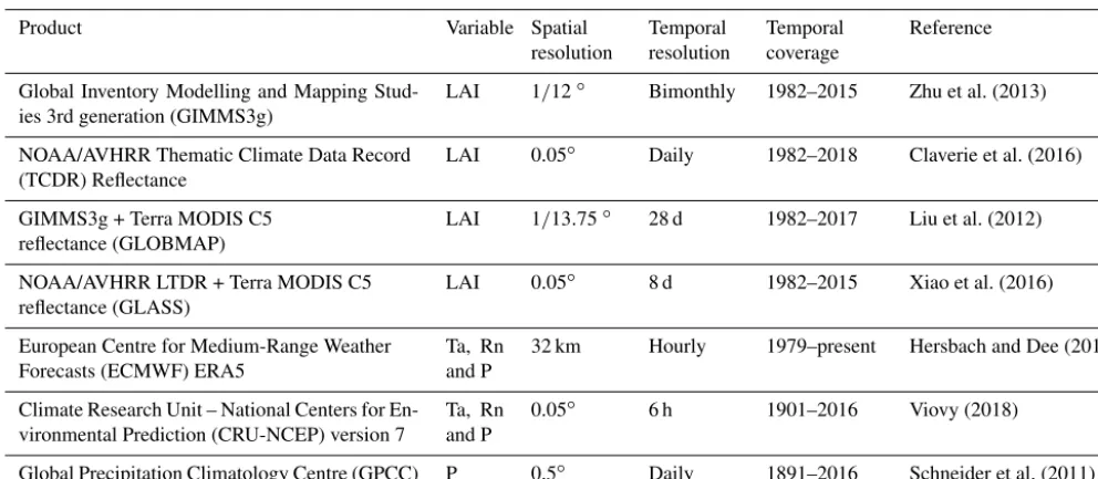
Table 1.Summary of global data sets used for vegetation, i.e. LAI, and climate, i.e. air temperature (Ta), net radiation (Rn), and precipitation (P).

Product Variable Spatial resolution Temporal resolution Temporal coverage Reference

Global Inventory Modelling and Mapping Stud-ies 3rd generation (GIMMS3g)

LAI 1/12◦ Bimonthly 1982–2015 Zhu et al. (2013)

NOAA/AVHRR Thematic Climate Data Record (TCDR) Reflectance

LAI 0.05◦ Daily 1982–2018 Claverie et al. (2016)

GIMMS3g + Terra MODIS C5 reflectance (GLOBMAP)

LAI 1/13.75◦ 28 d 1982–2017 Liu et al. (2012)

NOAA/AVHRR LTDR + Terra MODIS C5 reflectance (GLASS)

LAI 0.05◦ 8 d 1982–2015 Xiao et al. (2016)

European Centre for Medium-Range Weather Forecasts (ECMWF) ERA5

Ta, Rn and P

32 km Hourly 1979–present Hersbach and Dee (2016)

Climate Research Unit – National Centers for En-vironmental Prediction (CRU-NCEP) version 7

Ta, Rn and P

0.05◦ 6 h 1901–2016 Viovy (2018)

Global Precipitation Climatology Centre (GPCC) P 0.5◦ Daily 1891–2016 Schneider et al. (2011)

autocorrelation, has to be determined first, so it can later be factored out. At timet, the auto-predictive power ofY can be calculated with the following univariate autoregressive equa-tion:

yt= m

X

i=1

aiyt−i+t, (1)

where mdefines the maximum order of the autoregressive model (withm≤n),i is the time lag,ai represents the

co-efficients describing the linear interaction between different time steps, andt is the prediction error. Note that the order

mdefines the maximum lag that is investigated, which does not necessarily imply that all predictors have an effect up to time stepm. By increasingm, more lags are included, at the cost of increasing the computational demand.

The predictive power ofX onY can be assessed through construction of a second autoregressive model, containing a term capturing the contribution ofX, given by

yt= m

X

i=1

aiyt−i+ m

X

i=1

bixt−i+ηt, (2)

with ηt representing the prediction error of the bivariate

model. A drawback is the need to set the order m, which, if set to non-optimal, can result in large estimation errors.

Granger causality is then typically defined as the natural logarithm of the ratio of two prediction error variances (Ding et al., 2006),σ2andσ_η2for the univariate and bivariate mod-els, respectively:

GCX→Y =ln

σ2 σ2

η

. (3)

The null hypothesis ofX causingY (or vice versa), can be tested for significance against a presetpvalue, typically 5 %. Thus, if GCX→Y exceeds the preset threshold, assuring

that σ_η2 is significantly smaller than σ2, X is said to have a causal effect onY. Similarly, the causal effect ofY onX

can be determined. Note that as the effect of autocorrelation is removed, a simple correlation betweenXandY does not guarantee the presence of Granger causality as co-movement does not necessarily imply causality (Aldrich, 1995).

This framework can also be extended to the multivariate case, where the effect of predictorsX,Z1,Z2. . . Zp (with

p+1 the number of predictor variables) onY can be evalu-ated. In order to determine the effect ofXonY in a multivari-ate case, the performance of a model containing all predictors is compared against that of a multivariate model from which

Xis excluded, as given by

yt= m

X

i=1

aiyt−i+ p

X

j=1

(

m

X

i=1

bj,izj,t−i)+x,t, (4)

yt= m

X

i=1

aiyt−i+ p

X

j=1

(

m

X

i=1

bj,izj,t−i)+ m

X

i=1

cixt−i+ηt. (5)

The added value of incorporatingX in the set of predic-tors (Z1,Z2. . . Zp) to improve the prediction ofY can be

expressed in terms of Granger causality as GCX→Y =ln

σ2_x σ2

η

. (6)

2.2.2 Spectral Granger causality

se-J. Claessen et al.: Global biosphere–climate interaction 4855

ries to their seasonal and annual equivalents prior to follow-ing a traditional Granger causality approach does not neces-sarily lead to realistic causation inference at larger tempo-ral scales. Consequently, Granger causality frameworks that are defined in the time domain – such as the framework by Papagiannopoulou et al. (2017a) – are not designed to capture low-frequency processes. To assess temporal-scale-dependent processes, transforming the data into a frequency-dependent domain is crucial as it allows for a differentiation of interactions active at various temporal scales. Therefore, we propose the use of CSGC, which enables us to simul-taneously condition for other predictors, thus factoring out co-dependency among variables, while addressing processes active at different scales.

The spectral Granger causality (SGC) is a non-parametric extension of the Granger causality theory in which time se-ries are first transformed into a frequency domain, result-ing in a spectral analogue of Granger causality (Geweke, 1982). A well-known example of such a transformation is the Fourier transformation, where a time series is decomposed in a space solely consisting of frequency. This allows for highlighting strong spectral features, but comes at the cost of time localisation, i.e. the ability to differentiate between processes active at different times. To prevent the loss of the time dimension, SGC adopts a wavelet transformation, which decomposes the original time series into a time–frequency space, thus allowing for both spectral (i.e. temporal-scale-dependent) evaluation and time localisation of interactions between predictors and the target variable. In order to per-form the time–frequency decomposition, the Morlet wavelet is used and a balance between the time and frequency reso-lutions is obtained by setting the shape parameter to a value of 6, as in Torrence and Compo (1998) or Casagrande et al. (2015). Moreover, to overcome the limitation of assigning an arbitrary order of the system given by Eqs. (1) and (2), Dhamala et al. (2008) developed a non-parametric method to express spectral Granger causality based on spectral proper-ties of the variables without the need to estimate the model order, given by

SGCX→Y(f )=

ln Syy(f )

Syy(f )−

0xx−

02 yx

0yy

|Hyx(f )|2

, (7)

whereSyy(f )equals the spectral density (power spectrum)

of the target variable Y at frequency f, which can be es-timated from the wavelet transform. Using the variables X

andY, the error covariance matrix0and the spectral trans-fer function matrixH(f )can be calculated using matrix fac-torisation (Wilson, 1972). For more information on SGC, we refer to Ding et al. (2006), Dhamala et al. (2008), and Detto et al. (2012, 2013).

2.2.3 Conditional spectral Granger causality

Equation (7) is only valid to determine the effect of a vari-able X on Y, without taking into account that other vari-ables might influence both the predictor and target, conse-quently inducing an apparent causal relationship. To tackle this issue, conditionality between variables has to be taken into account, for which the SGC framework can be ex-tended to the conditional spectral Granger causality (CSGC). In other words, SGC can be adapted to CSGC to assess if X causes Y given that Z1, Z2. . .Zp may cause Y and

X, resulting in a conditioned measure of spectral causal-ity CSGCX→Y|Z1,Z2...Zp(f ). For a multivariate problem with p+2 variables (Y,X,Z1,Z2. . .Zp), the system can be written,

after spectral transformation and Wilson factorisation (Wil-son, 1972), as

S(Y, X, Z1, Z2. . .Zp, f )=H(f )6H∗(f ), (8)

U(Y, Z1, Z2. . .Zp, f )=G(f )0G∗(f ), (9)

withSandUrepresenting the spectral matrices of the com-plete system and the system with the variable whose causal-ity is tested being excluded, i.e.Xin this case, respectively. Similarly,HandGare the spectral transfer function matri-ces, while6 and0equal the error covariance matrix of the full and incomplete systems of variables, respectively, and where∗indicates matrix adjoint.

From Eqs. (8) and (9), CSGC ofXonY givenZ1,Z2. . .

Zpcan be calculated as

CSGCX→Y|Z1,Z2...Zp(f )=ln

0yy

|Qyy(f )6xxQ∗yyf|

, (10) where: Q=       e

GY Y 0 GeY Z1 . . . GeY Zp

0 1 0 . . . 0

e

GZ1Y 0 GeZ1Z1 . . . GeZ1Zp

. . . .

e

GZpY 0 GeZpZ1 . . . GeZpZp

      −1 ×       e

HY Y HeY X . . . HeY Zp

e

HXY . . . .

. . . . . . . .

e

HZpY HeZpX . . . HeZpZp

      . (11)

In Eq. (11),eH(f )=H(f )P−1andeG=GP−₂1represent

cor-rected transfer function matrices to separate the directional interactions (Geweke, 1982). The rotation matricesPare nor-malisation matrices needed to transform the multivariate sys-tems in their canonical form with uncorrelated errors (Detto et al., 2013). For more information on CSGC, we refer to Dhamala et al. (2008) and Detto et al. (2012, 2013).

Using Eq. (10), conditional spectral Granger causality of

. . . Zp on both X andY. If X is not directly affecting Y,

but for example Z1 is forcing both X andY, the numera-tor in Eq. (10) will equal the denominanumera-tor, thus resulting in a Granger causality measure of zero. However, if there is a direct causal influence ofXonY at a specific frequencyf, CSGCX→Y|Z1,Z2...Zp(f ) >0. Using Eq. (10), it is possible to determine ifX(Granger) causesY, but no information on the sign of the causal relation can be extracted.

2.2.4 Significance testing of CSGC

Despite the ability of Eq. (10) to account for conditional ef-fects between variables, it fails to determine how robust the found interactions are. Therefore, the robustness of the de-termined CSGC values needs to be tested against the null hypothesis thatXhas no causal effects onY. In the case of Granger causality in the time domain, significance of the de-termined statistic, e.g. Granger causality (GC), can be tested by a bootstrapping scheme in which the time series are ran-domly shuffled before determining the GC values. By repeat-ing this procedurentimes, the distribution of GC can be de-termined. By selecting a p value, typically 5 %, the deter-mined Granger causality ofXonY can be tested against the null hypothesis of no causal interaction.

However, for the spectral variant of Granger causality, a simple randomisation of the time series induces unwanted artefacts. Due to the spectral nature of the method, the power spectrum of the randomised time series must be preserved, i.e. to be equal to that of the original time series at each fre-quency. In other words, if the original time series are char-acterised by much high-frequency variation and less at lower frequencies, the time series used for significance testing need to show the same frequency-dependent variability. Therefore, surrogate time series exhibiting the same spectral power as the original time series need to be used. Here, iterative am-plitude adjusted Fourier transform (IAAFT) surrogates are used in combination with Monte Carlo simulations, as CSGC is non-parametric (Detto et al., 2012), to test the determined CSGC value against the null hypothesis of no causal inter-action. Due to computational constraints, 100 runs with sur-rogates were performed for each set of original time series (i.e. for each pixel) and will be used to test for significance (pvalue<0.05). However, to increase the robustness of the results, an ensemble of products is used for both the observa-tions and models as explained in Sect. 2.1.

2.2.5 Explained variance

CSGC, as defined by Eq. (10), compares the performance of two autoregressive models in explaining variation in a target variable Y. In other words, does X, given a set of predic-tors Z1,Z2. . . Zp, improve the estimate ofY compared to

a model that only usesZ1,Z2. . . Zp? In this study, we are

interested in quantifying how much of variance in the target variable is actually directly explained by a predictor and not

how much the estimation error improved upon addingXto the set of the predictors. Therefore, we deviate from the tra-ditional formulation of Granger causality and define a new measure, the fraction (F) of variance in the target variableY

that is explained by a predictorX. Ideally, the new formula-tion would be

FX→Y =

σ_X2 σ_Y2

×100 %, (12)

withσ_Y2representing the total variance ofY andσ_X2the vari-ance inY explained byX. However, a part of the variance in

Y is not explainable by any predictor, as is forced by the au-tocorrelation ofY(σ_Y,2_auto). Therefore, in order to account for the part of variance inY that will not be able to be explained by any predictor, Eq. (12) is adapted to

FX→Y =

σ_X2 σ_Y2−σ_Y,2_auto

×100 %. (13)

As traditional Granger causality and CSGC determine a mea-sure of causality that is defined in a similar way, Eq. (1) can be used to determine howF can be calculated from the actual Granger causality value. Considering the univariate model given by Eq. (1), the total variance in the target variableY

can be rewritten as

σ_Y2=σ_Y,2_auto+σ2, (14)

withσ2representing the unexplained variance or prediction error variance. Substituting Eq. (14) into Eq. (13) results in

FX→Y =

σ_X2 σ2

×100 %. (15)

This derivation can also be extended towards the multivariate case and even to CSGC. As Eq. (15) equals 1−e−GCX→Y_, the conditional spectral variant of the fraction of variance in

Y explained byXcan be calculated as

FX→Y|Z1,Z2...Zp(f )=

0yy− |Qyy(f )6xxQ∗yyf|

0yy

×100 %. (16)

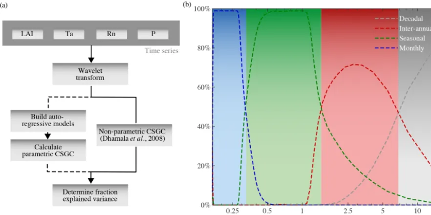
Using Eq. (16), the impact of climate on vegetation and the feedbacks of vegetation on climate can be quantified and re-ported in an intuitive manner (see Fig. 1a and Sect. 3). 2.2.6 Determining scales of interest

J. Claessen et al.: Global biosphere–climate interaction 4857

Figure 1. (a)Schematic overview of CSGC, extended by the calculation of the fraction of explained variance.(b)Scales affected by pertur-bation of variability in synthetic time series at a particular temporal scale. Coloured lines show, for each perturbed variability, the scales that changed most compared to the unperturbed runs as a percentage of runs out of 100 000. The shaded colours indicate the ranges adopted for each temporal scale in the analysis.

differ from the short-term processes. Hereafter, the terms

phenology andphenological cycle are used to refer to the seasonal-scale variability in LAI. This reflects features such as the timing of the growing season or the amplitude of the intra-annual cycle (Richardson et al., 2009; Verger et al., 2016) since CSGC will react to variability in both the time and frequency domains. As explained in Sect. 2.2.3, CSGC allows a simultaneous analysis of the interactions at multi-temporal scales, while no assumption needs to be made about the direction of the interplay between climate and vegetation. Moreover, based on the characteristics of the climate data used in this study, CSGC can be applied to assess causality over a wide range of temporal scales, starting at 2 months (twice the temporal resolution) and going up to 16.5 years (maximum temporal scale due to discretisation of the fre-quency space; can be adjusted if needed, especially for longer time series).

In order to determine which range of temporal scales better represents monthly, seasonal, and inter-annual interactions, an experiment with synthetic monthly time series was per-formed. First, a predictor variable (X1) is constructed with imposed variability at the scales of interest (e.g. monthly, seasonal, and inter-annual). Monthly variability is assumed to be random from month to month, while seasonality is de-fined as consecutive three-block periods of a constant value. Inter-annual variation is defined as blocks of 1 year with a fixed value. The predictor X1 is constructed by randomly generating these three variabilities and adding them. Finally, a linear trend is added toX1to be able to retrieve the

maxi-mum scale at which inter-annual variability can be observed. Next, a target variable (Y1) is constructed with a known causal relation to the predictorX1 by multiplyingX1 with a random factor and then shiftingY1in time so thatY1lags

X1by 1 month. Using these two synthetic time series, SGC is used to determine the Granger causality ofX1onY1. Note that SGC is used instead of CSGC as the scales at which the targeted interactions can be observed are identical for the bi-variate and multibi-variate cases.

In order to identify the scales that are most sensitive to monthly, seasonal, and inter-annual interactions, a new pre-dictor variableX2is constructed as an identical copy ofX1, except for one specific variability. For example, if the range of scales that capture monthly interactions is determined,X2 will be equal toX1, but with perturbed monthly variability. Next, a new target variableY2is constructed by multiplying

can-not be investigated here due to length of the observational record (see Sect. 2.1), but they are used in the determination of the ranges to fix the upper limit for inter-annual interac-tions. See Fig. 1b for an illustration of the resulting scales, which are considered to be time- and space-invariant. Re-sults will be presented as mean patterns for each scale us-ing the determined ranges. Selectus-ing the maximum explained variance within each range, unwillingly results in taking the CSGC at the highest scale of each interval, as the CSGC in-creases with the scale (for more information, see Sect. 3.1).

3 Results and discussion

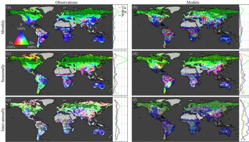
3.1 Climate impact on vegetation in observations Figure 2a, c, and e illustrate the Granger causality of air temperature, net radiation, and precipitation on LAI dynam-ics, based on observations, globally and latitudinally. Re-sults are shown separately for monthly (Fig. 2a), seasonal (Fig. 2c), and inter-annual (Fig. 2e) timescales using a tri-variate colour map according to the fraction explained by each climatic driver (see Sect. 2.2.5). Dotted pixels indi-cate that in at least 75 % of the ensemble members there is (a) agreement regarding the dominant climate impact and (b) statistical significance (at the 5 % level). At monthly scales, overall spatial patterns in the observation-based re-sults (Fig. 2a) are in agreement with previous studies, show-ing the dominance of precipitation in arid and semi-arid re-gions, while radiation and temperature dominate in northern latitudes and rainforests, respectively (Nemani et al., 2003; de Jong et al., 2013; Seddon et al., 2016; Papagiannopoulou et al., 2017b). Strong radiation effects on vegetation can be observed over northern latitudes due to severe limitations in incoming radiation during winter months. However, in those latitudes, LAI retrievals are contaminated by snow cover sig-nals. While focusing on the growing season could solve this issue, the CSGC requires continuous time series. Because in wintertime, due to limitations in solar radiation, plant growth is inhibited in northern latitudes, most variability captured at monthly scales will be dominated by the more dynamic spring and summer periods; therefore, our results suggest that radiation still dominates the behaviour of vegetation at these latitudes.

This dominant high-latitude radiation control was not re-ported by Papagiannopoulou et al. (2017b), who, based on a non-linear Granger causality framework, found that 61 % of the vegetated land surface is primarily driven by water avail-ability at monthly timescales, while temperature and radia-tion are the primary factors in only 23 % and 15 % of the vegetated surface, respectively. These results also contrasted with earlier studies, which pointed to a less dominant role of water availability for global ecosystems (Nemani et al., 2003; Wu et al., 2015). Here, our monthly-scale results also show a dominant role of precipitation, yet more moderate; 51 %

of vegetated land is primarily controlled by precipitation, with radiation being the primary control factor in 40 % as well. When the analysis targets vegetation anomalies by de-trending linearly and subtracting the average seasonal cycle for both LAI and climate (as was done in Papagiannopoulou et al., 2017a, b), results show a similar dominance of precip-itation, but air temperature gains importance over net radia-tion (being the dominant driver over 13 % and 36 %, respec-tively, as indicated in Fig. A1 in Appendix A). The higher importance of water availability in Papagiannopoulou et al. (2017b) can be attributed to accounting directly for the ef-fect of (root depth) soil moisture as a driver of vegetation, as opposed to the use of precipitation only in this study. Also, human practices, such as irrigation, can potentially bias our results. Nonetheless, irrigation is expected to increase the en-ergy dependence of LAI dynamics, and as irrigation tends to be a seasonal phenomenon restricted to the growing period, this increase is found to be clearer at seasonal than monthly scales (as shown in Fig. B1 in Appendix B). A final differ-ence with Papagiannopoulou et al. (2017b) is their consider-ation of snow water equivalent as a water availability driver, which explains the divergence with our results in higher lati-tudes. Our results can also be reconciled with previous stud-ies, such as Nemani et al. (2003), Wu et al. (2015), and Sed-don et al. (2016); regional differences may relate to the spe-cific focus of those studies on one temporal scale only, their calculation of covariances instead of inferring causality in a more formal manner, or the use of different variables to as-sess water availability drivers.

J. Claessen et al.: Global biosphere–climate interaction 4859

Figure 2.Global climate impact on vegetation. Variability in(a, c, e)observed and(b, d, f)modelled LAI caused by air temperature (Ta), net radiation (Rn), and precipitation (P) at(a, b)monthly,(c, d)seasonal, and(e, f)inter-annual timescales. Maps show the causality in relative terms with respect to the dominant driver at each pixel, while the latitudinal profiles show the absolute impact of each driver. The period 1982–2015 is taken as reference for the observations, while models span 1956–2005. Maps show the mean from the ensemble of the observations for four CMIP5 models: CCSM4, HadGEM2-ES, NorESM1-M, and IPSL-CM5A-MR. Dotted pixels indicate a significant (pvalue=5 %) primary driver agreed upon by at least 75 % of the ensemble members.

Finally, at inter-annual scales, despite co-dominance of multiple drivers in some regions, global ecosystems tend to be water limited with 43 % of the vegetated land surface being primarily dominated by precipitation (Fig. 2e), espe-cially in the subtropics. Although patterns exhibit some het-erogeneity, not only arid and semi-arid regions but also sub-stantial parts of southern Eurasia show a (significant) domi-nant control by precipitation. This widespread inter-annual dependency on water availability of ecosystem dynamics may arise due to the large inter-annual variability of pre-cipitation and has already been documented in relation to the impact of precipitation of global carbon budgets (Poul-ter et al., 2014) and (Poul-terrestrial evaporation (Miralles et al., 2014). Moreover, it agrees with the results of Green et al. (2019) and Humphrey et al. (2018), yet it does not nec-essarily contradict the findings by Jung et al. (2017). Jung et al. (2017) reported a dominant role of temperature at the global scale, yet showed a dominance of water availability at regional scales that is compensated for when upscaling to global means. Inter-annually, the control of air temper-ature extends over the high northern latitudes and eastern China, dominating in 20 % of vegetated land, while radia-tion remains the most crucial driver for 37 % of the land

surface, almost exclusively in the northern latitudes, likely affected by the strong seasonal patterns (Fig. 2e). Once the seasonality is removed, the inter-annual dominance of radia-tion control falls down to 20 % of the vegetated land surface (see Fig. A1c). Despite the heterogeneity, the overall con-trol of climate on vegetation is higher at inter-annual scales than at shorter timescales, as can be observed in the latitudi-nal profiles, which show the total causality in absolute terms (Fig. 2). This is partly a consequence of the time–frequency decomposition of CSGC, which generally results in higher values of explained variance at longer timescales due to the increased time frame over which a predictor variable is as-sessed, thus increasing the chance of incorporating memory effects. However, the significance test against the null hy-pothesis of exhibiting no causal effect ensures that regions exhibiting significant responses can be compared over differ-ent timescales.

to reduced plant transpiration, which in turn may induce a decline in precipitation, creating a warmer and drier regime (Lawrence and Vandecar, 2015). Irrigation allows for grow-ing crops in water-limited regions, consequently inducgrow-ing en-ergy constraints which are captured by the CSGC. Note that due to the limited data record, the effects of global warming trends and carbon dioxide fertilisation – and the consequent trends in vegetation greening and water use efficiency (Re-ichstein et al., 2013; Wu et al., 2015; Zhu et al., 2016) – are not directly addressed in this study.

3.2 Climate impact on vegetation in models

Results of the observations are next used to benchmark CMIP5 ESM performance in representing the control of cli-mate on vegetation (Fig. 2b, d, f). Dotted pixels indicate that at least three out of four models reach agreement regarding (a) dominant climate impact and (b) statistical significance (at the 5 % level). Comparison of Fig. 2a and b shows that the monthly impact of air temperature on ecosystems is strongly overestimated by ESMs, with 17 % and 26 % of vegetated land being primarily dominated by temperature for observa-tions and ESMs, respectively. This coincides with a lower effect of net radiation in central Eurasia and, more impor-tantly, elevated air temperature control in the Amazon and Congo rainforests. These contrasting results with observa-tions might hint towards problems in ESMs with respect to representing the behaviour of the tropics but may also re-late to the difficulties to retrieve LAI from satellites in dense forests (Hilker et al., 2015). Nevertheless, ESMs agree on the general patterns that highlight the strong radiation ef-fects in northern latitudes (albeit less extended) and the water availability as a main driver in arid and semi-arid regions at monthly timescales.

Seasonally, a larger control of precipitation and air tem-perature on vegetation phenology is also noticeable over the Equator for ESMs (see latitudinal profile in Fig. 2d). The dominant control of radiation on vegetation phenology over northern latitudes is similar for all models (inter-model agreement and significance represented by the black dotting), and, whereas the spatial extent agrees with the observational results, the magnitude is underestimated by the models (see Fig. 2c and d). Radiation is the primary driver of the sea-sonal LAI variation in 45 % of the vegetated land in models (compared to 55 % for the observations). The role of pre-cipitation and air temperature as drivers of the phenologi-cal cycle gains in importance in ESMs, at the cost of radi-ation, with 40 % and 15 % of seasonal LAI variation being dominated by precipitation and air temperature variability, respectively, versus the 33 % and 12 % in observations, re-spectively. Despite the overall similarities in the patterns of dominant drivers, regional differences between observations and models are still observed. Models point towards a water-limited phenological cycle in the Sahel, while observations also hint at a dominant role of temperature (compare Fig. 2c

and d). Furthermore, whereas observations clearly highlight a south-to-north water-to-energy-limited gradient in Ama-zonia, models tend to disagree and point towards tempera-ture as a key driver over most of the Amazonian rainforest at seasonal scales. These differences might indicate difficul-ties to model climate–vegetation interactions across the basin where air temperature is found to be the only limiting con-trol, yet they may again be influenced by the difficulties to retrieve LAI from satellites over dense canopies, as pointed out above.

Similar to observations, the climate impact on LAI in-creases with longer temporal scales in ESMs. However, more remarkable than in the observations is the strong water lim-itation across the globe at inter-annual scales, which is not restricted to arid and semi-arid regions (Fig. 2f). Water avail-ability at inter-annual scales is dominant for vegetation over 62 % of land versus the 43 % found in observations (Fig. 2e) and is also strongly overestimated in absolute terms at most latitudes, especially in the tropics. Further analysis shows that the divergence in the considered period between obser-vations and models (see Sect. 2.1) does not substantially im-pact results; repeating the analysis for the overlapping time range for observations and models (1982–2005) yields very similar findings (Fig. D1 in Appendix D).

3.3 Vegetation feedback on climate in observations and models

Analogous to the effect of climate on vegetation, vegetation can alter local (and remote) climate conditions via biophys-ical and biochembiophys-ical feedbacks. These feedbacks arise from the effect of vegetation structure and physiological activity on the surface radiation budget, available energy partition-ing into latent and sensible heat fluxes, aerodynamic conduc-tance of the ecosystem, atmospheric chemical composition, and indirect processes affecting incoming radiation, atmo-spheric humidity, and temperature (McPherson, 2007; Bo-nan, 2008). The representation of these feedbacks in ESMs remains in need of improvement to accurately predict fu-ture climate (de Noblet-Ducoudré et al., 2012; Zhang et al., 2016). Here, we unravel these feedbacks of LAI on differ-ent climate variables based on observations (Fig. 3a, c, and e) and ESM data (Fig. 3b, d, and f) and at different temporal scales, from monthly (Fig. 3a and b) to seasonal (Fig. 3c and d) and inter-annual (Fig. 3e and f). Dotted pixels indicate that in at least 75 % of the ensemble members there is (a) agree-ment regarding the dominant feedback and (b) statistical sig-nificance (at the 5 % level). To aid comparison to the strength of climate impacts on vegetation – measured in relative or absolute percentage of caused variance (see Sect. 2.2.5) – an identical tri-variate colour map to that in Fig. 2 is used.

reflec-J. Claessen et al.: Global biosphere–climate interaction 4861

Figure 3.Global vegetation feedback on climate. Variability in air temperature (Ta), net radiation (Rn), and precipitation (P) that is caused by(a, c, e)observed and(b, d, f)modelled LAI at(a, b)monthly,(c, d)seasonal, and(e, f)inter-annual timescales. Maps show the causality in relative terms with respect to the strongest feedback at each pixel, while the latitudinal profiles show the absolute feedback on each driver. The period 1982–2015 is taken as reference for the observations, while models span 1956–2005. Maps show the mean from the ensemble for observations for four CMIP5 models: CCSM4, HadGEM2-ES, NorESM1-M, and IPSL-CM5A-MR. Dotted pixels indicate the significant (pvalue=5 %) strongest feedback agreed upon by at least 75 % of the ensemble members.

tion back into the atmosphere; this increases surface net radi-ation and may lead to a net warming effect (e.g. Bonan, 2008; Forzieri et al., 2017). By repeating the analysis using only in-coming (shortwave and longwave) radiation, instead of sur-face net radiation, the results indicate that the influence of LAI on cloud formation is limited, at least considering the lo-cal (in the sense of “spatially collocated”) slo-cales revealed by the causal framework (see Fig. E1 in Appendix E). Monthly feedbacks of vegetation on precipitation and air temperature are spatially less widespread; however, significant feedbacks on precipitation are observed, especially in tropical forests. The patterns in Amazonia suggest a more dominant effect of vegetation on radiation in the north, while precipitation feedbacks dominate in the south (Fig. 3a). We note that the method does not differentiate whether higher or lower val-ues of LAI cause more or less rainfall, only that a causal effect of LAI on rainfall exists. The south-to-north patterns in the Amazon agree with the larger dependency on precip-itation recycling in the south (Dirmeyer et al., 2009; Zemp et al., 2014). Tropical forests are known to regulate local (and global) precipitation as their large use of water increases at-mospheric humidity and results in cloud formation (Malhi et al., 2008). This also directly affects the incoming

short-and long-wave radiation. Nevertheless, we restate that the method only focuses on the effects of LAI on its immedi-ate climatic environment, not in neighbouring or remote lo-cations.

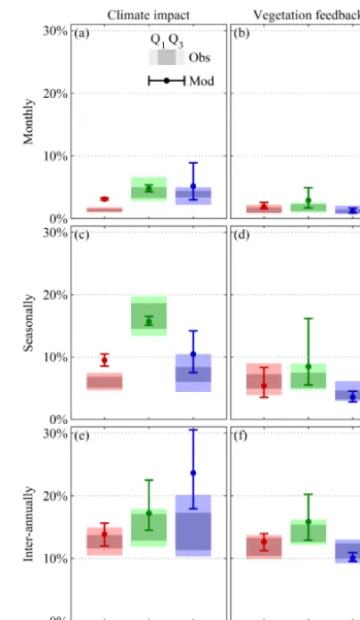
Figure 4.Climate impact on vegetation per biome. Biome averages of absolute observed (filled polygons) and modelled (lines) variation in LAI caused by air temperature (Ta), net radiation (Rn), and precipitation (P), at monthly(a, b, c), seasonal(d, e, f), and inter-annual(g, h i) timescales. Observations present the total range over all ensemble members and the 25th (Q1) and 75th percentiles (Q3). Models present an error bar indicating the inter-model maximum, minimum, and average results of four CMIP5 models (CCSM4, HadGEM2-ES, NorESM1-M, IPSL-CM5A-MR). Represented biomes are mixed forests (MF), deciduous broadleaf forest (DBF), deciduous needleleaf forest (DNF), evergreen broadleaf forest (EBF), evergreen needleleaf forest (ENF), barren or sparsely vegetated (BSV), cropland or natural vegetation mosaic (CNVM), croplands (C), grasslands (G), savannas (S), woody savannas (WS), and open shrublands (OS).

vegetation consistently exceeds the strength of the vegetation feedback on climate. This means that local climate variability leaves a larger imprint on LAI dynamics than vice versa. This can be partly attributed to the fact that only local interactions are considered here: while vegetation reacts to its most im-mediate environment, vegetation can lead to remote effects on climate that are not addressed in our analyses (Dirmeyer et al., 2009; Miralles et al., 2019). Nevertheless, these results show the importance of LAI variability in explaining the vari-ance in local climate at intra-annual scales – mainly through impacts on the net radiation induced by albedo changes – and the potential of the CSGC framework to disentangle the bidirectional interaction between vegetation and climate.

In general, ESMs seem to correctly capture the spatial ex-tent of LAI effects on net radiation throughout most of the

J. Claessen et al.: Global biosphere–climate interaction 4863

Figure 5.Vegetation feedback on climate per biome. Biome averages of absolute observed (filled polygons) and modelled (lines) variation in air temperature (Ta), net radiation (Rn), and precipitation (P) caused by LAI, at monthly(a, b, c), seasonal(d, e, f), and inter-annual(g, h i) timescales. Observations present the total range over all ensemble members and the 25th (Q1) and 75th percentiles (Q3). Models present an error bar indicating the inter-model maximum, minimum, and average results of four CMIP5 models (CCSM4, HadGEM2-ES, NorESM1-M, IPSL-CM5A-MR). Represented biomes are mixed forests (MF), deciduous broadleaf forest (DBF), deciduous needleleaf forest (DNF), evergreen broadleaf forest (EBF), evergreen needleleaf forest (ENF), barren or sparsely vegetated (BSV), cropland or natural vegetation mosaic (CNVM), croplands (C), grasslands (G), savannas (S), woody savannas (WS), and open shrublands (OS).

suggest a lower dependency of tropical forests on rainfall re-cycling (Malhi et al., 2008; Hilker et al., 2014; Zemp et al., 2017) and/or an overall wet bias in the ESMs (Mueller and Seneviratne, 2014); the latter is however not supported by the results in Fig. 2 that indicate an overall overestimation of water limitations in models. Nonetheless, these local feed-backs on temperature and precipitation are overall weak – in both observations and models – as indicated by the absolute magnitudes shown in the latitudinal profiles (Fig. 3). 3.4 Biome-specific interactions

Finally, to better visualise the multi-temporal-scale vegetation–climate interactions in observations and models, results are presented averaged per biome type. Figure 4

the minimum modelled temperature control. Interestingly, models also overestimate the sensitivity of broadleaf forests (EBF and DBF) to precipitation, especially at inter-annual timescales. Observation results show limited water stress in tropical and mid-latitude forests, arguably due to the deep rooting system and mild climate. However, this apparent model overdependency of broadleaf forests on climate may also emerge from the under-sensitivity of the observational results due to the saturation of the greenness signal received by satellites in dense canopies. Models unambiguously overestimate the importance of water availability for LAI in most biome types at inter-annual timescales and to a more limited extent at monthly and seasonal scales – this appears in contrast with the results of Green et al. (2017). As expected, savannas are found to be mainly driven by precipitation across all timescales in both observations and models, although models strongly disagree among each other, as reflected by the large error bars in Fig. 4.

On the other hand, short-term feedbacks of LAI on climate seem to be better represented in ESMs, as small differences can be seen when compared to the observational results in Fig. 5. Note that this statement only holds true if looking at biome-averaged patterns due to compensatory effects, as comparison of observations and models in Fig. 3 does indi-cate clear regional differences. Deciduous needleleaf forests (DNF) and evergreen needleleaf forests (ENF) exhibit the strongest feedback on net radiation (and temperature) at all temporal scales; once again this appears related to albedo changes and not impacts on cloud formation (see Fig. E1). Nonetheless, the effect of needleleaf forests on the radiation budget tends to be overestimated by most CMIP5 models, especially at monthly and seasonal timescales, which aligns with the findings of Forzieri et al. (2018). ESMs also overes-timate the influence of ecosystem phenology on net radiation in mixed forests (MF), open shrublands (OS), and woody sa-vannas (WS); yet, large inter-model disagreements exist on the seasonal influence of LAI on net radiation for almost all biomes, as illustrated by the large error bars in Fig. 5. The strength of the effect of LAI on precipitation is overall lower than its impact on net radiation and air temperature, partly due to the non-consideration of downwind influences, which have been shown to be crucial, in this analysis (Dirmeyer et al., 2009; Zemp et al., 2017). However, similar to the re-sults of Green et al. (2017), a strong influence of LAI on precipitation can be observed in savannah regimes.

4 Conclusion

Here, bidirectional interactions between climate and vegeta-tion in global remotely sensed observavegeta-tions were analysed at different temporal scales using conditional spectral Granger causality (CSGC) with the aim to benchmark the represen-tation of these interactions in ESMs. Three main climate variables are considered, namely air temperature, net

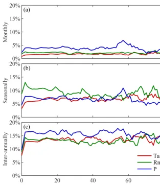
radi-Figure 6.Global average climate impact on vegetation and vege-tation feedback on climate. Global averages of absolute observed (filled rectangles) and modelled (lines) variation in vegetation(a, c, e)(climate(b, d, f)) caused by climate (vegetation), at monthly(a, b), seasonal(c, d), and inter-annual(e, f)timescales. Models present an error bar indicating the inter-model maximum, minimum, and average results of four CMIP5 models (CCSM4, HadGEM2-ES, NorESM1-M, IPSL-CM5A-MR).

J. Claessen et al.: Global biosphere–climate interaction 4865

generally overestimate the precipitation control on vegeta-tion and most drastically at inter-annual scales. On the other hand, vegetation feedbacks are found to be locally more pre-dominant for net radiation over all timescales, mainly due to the strong interplay between radiation and vegetation at northern latitudes. As shown by the summary in Fig. 6, ESMs tend to overestimate the feedbacks on the radiation budget, while feedbacks on local precipitation are often underesti-mated, especially at seasonal and inter-annual scales. Finally, interactions in both ways are found to increase with increas-ing timescales, and feedbacks of vegetation on climate ex-plain a lower fraction of the variance in climate than vice versa.

Appendix A: Climate impact on vegetation in anomalies of observations

J. Claessen et al.: Global biosphere–climate interaction 4867 Appendix B: Climate impacts on vegetation as a

function of irrigation for observations

Appendix C: Climate impact on vegetation in observations using incoming radiation instead of net radiation

J. Claessen et al.: Global biosphere–climate interaction 4869 Appendix D: Climate impact on vegetation in

observations and ESMs during 1982–2005

Appendix E: Vegetation feedback on climate in observations using incoming radiation instead of net radiation

J. Claessen et al.: Global biosphere–climate interaction 4871

Code availability. Our scripts can be accessed via https://github. com/lhwm/ConditionalSpectralGrangerCausality (Claessen et al., 2019).

Author contributions. DGM and JC conceived the study and led the writing. JC conducted the analysis. MDem contributed to the data-processing. AM and MDet contributed to the implementation of the method. All co-authors contributed to the design of the experiments, interpretation of results, and editing of the paper.

Competing interests. The authors declare that they have no conflict of interest.

Acknowledgements. This work is funded by the Belgian Science Policy Office (BELSPO) in the framework of the STEREO III programme, projects SAT-EX (SR/00/306) and SAT-EX Wave (SR/02/367). Diego G. Miralles acknowledges funding from the European Research Council (ERC) under grant agreement 715254 (DRY–2–DRY). We acknowledge the World Climate Research Pro-gramme’s Working Group on Coupled Modelling, which is respon-sible for CMIP. We also thank the climate modelling groups for their effort in producing and making available their model output.

Review statement. This paper was edited by Alexey V. Eliseev and reviewed by Giovanni Forzieri and one anonymous referee.

References

Aldrich, J.: Correlations genuine and spurious in Pearson and Yule, Stat. Sci., 10, 364–376, 1995.

Alessandri, A., Catalano, F., De Felice, M., Van Den Hurk, B., Reyes, F. D., Boussetta, S., Balsamo, G., and Miller, P. A.: Multi-scale enhancement of climate prediction over land by increasing the model sensitivity to vegetation variability in EC-Earth, Clim. Dynam., 49, 1215–1237, 2017.

Alkama, R. and Cescatti, A.: Biophysical climate impacts of recent changes in global forest cover, Science, 351, 600–604, 2016. Anav, A., Murray-Tortarolo, G., Friedlingstein, P., Sitch, S., Piao,

S., and Zhu, Z.: Evaluation of land surface models in reproducing satellite derived leaf area index over the high-latitude northern hemisphere. Part II: Earth system models, Remote Sensing, 5, 3637–3661, 2013.

Anav, A., Friedlingstein, P., Beer, C., Ciais, P., Harper, A., Jones, C., Murray-Tortarolo, G., Papale, D., Parazoo, N. C., Peylin, P., Piao, S., Sitch, S., Viovy, N., Wiltshire, A., and Zhao, M.: Spa-tiotemporal patterns of terrestrial gross primary production: A review, Rev. Geophys., 53, 785–818, 2015.

Bentsen, M., Bethke, I., Debernard, J. B., Iversen, T., Kirkevåg, A., Seland, Ø., Drange, H., Roelandt, C., Seierstad, I. A., Hoose, C., and Kristjánsson, J. E.: The Norwegian Earth Sys-tem Model, NorESM1-M – Part 1: Description and basic evalu-ation of the physical climate, Geosci. Model Dev., 6, 687–720, https://doi.org/10.5194/gmd-6-687-2013, 2013.

Bonan, G. B.: Forests and climate change: forcings, feedbacks, and the climate benefits of forests, Science, 320, 1444–1449, 2008. Casagrande, E., Mueller, B., Miralles, D. G., Entekhabi, D., and

Molini, A.: Wavelet correlations to reveal multiscale coupling in geophysical systems, J. Geophys. Res.-Atmos., 120, 7555–7572, 2015.

Chen, C., Park, T., Wang, X., Piao, S., Xu, B., Chaturvedi, R. K., Fuchs, R., Brovkin, V., Ciais, P., Fensholt, R., Tømmervik, H., Bala, G., Zhu, Z., Nemani, R. R., and Myneni, R. B.: China and India lead in greening of the world through land-use manage-ment, Nature Sustainability, 2, 122–129, 2019.

Claessen, J., Molini, A., Martens, B., Detto, M., Demuzere, M., and Miralles, D. G.: Source code: Conditional spec-tral Granger causality, available at: https://github.com/lhwm/ ConditionalSpectralGrangerCausality, last access: 17 December 2019.

Claverie, M., Matthews, J., Vermote, E., and Justice, C.: A 30+ year AVHRR LAI and FAPAR climate data record: Al-gorithm description and validation, Remote Sensing, 8, 263, https://doi.org/10.3390/rs8030263, 2016.

Collins, W. J., Bellouin, N., Doutriaux-Boucher, M., Gedney, N., Halloran, P., Hinton, T., Hughes, J., Jones, C. D., Joshi, M., Lid-dicoat, S., Martin, G., O’Connor, F., Rae, J., Senior, C., Sitch, S., Totterdell, I., Wiltshire, A., and Woodward, S.: Development and evaluation of an Earth-System model – HadGEM2, Geosci. Model Dev., 4, 1051–1075, https://doi.org/10.5194/gmd-4-1051-2011, 2011.

de Jong, R., Schaepman, M. E., Furrer, R., De Bruin, S., and Verburg, P. H.: Spatial relationship between climatologies and changes in global vegetation activity, Glob. Change Biol., 19, 1953–1964, 2013.

De Keersmaecker, W., Lhermitte, S., Tits, L., Honnay, O., Somers, B., and Coppin, P.: A model quantifying global vegetation re-sistance and resilience to short-term climate anomalies and their relationship with vegetation cover, Global Ecol. Biogeogr., 24, 539–548, 2015.

de Noblet-Ducoudré, N., Boisier, J.-P., Pitman, A., Bonan, G., Brovkin, V., Cruz, F., Delire, C., Gayler, V., Van den Hurk, B., Lawrence, P., van der Molen, M. K., Müller, C., Reick, C. H., Strengers, B. J., and Voldoire, A.: Determining robust impacts of land-use-induced land cover changes on surface climate over North America and Eurasia: results from the first set of LUCID experiments, J. Climate, 25, 3261–3281, 2012.

Detto, M., Molini, A., Katul, G., Stoy, P., Palmroth, S., and Baldoc-chi, D.: Causality and persistence in ecological systems: a non-parametric spectral Granger causality approach, Am. Nat., 179, 524–535, 2012.

Detto, M., Bohrer, G., Nietz, J., Maurer, K., Vogel, C., Gough, C., and Curtis, P.: Multivariate conditional Granger causality analy-sis for lagged response of soil respiration in a temperate forest, Entropy, 15, 4266–4284, 2013.

Dhamala, M., Rangarajan, G., and Ding, M.: Estimat-ing Granger causality from Fourier and wavelet trans-forms of time series data, Phys. Rev. Lett., 100, 018701, https://doi.org/10.1103/PhysRevLett.100.018701, 2008. Ding, M., Chen, Y., and Bressler, S. L.: Granger Causality: Basic

Applica-tions, edited by: Schelter, B., Winterhalder, M., and Timmer, J., Weinhein, Germany: Wiley-VCH Verlag, 437–460, 2006. Dirmeyer, P. A., Brubaker, K. L., and DelSole, T.: Import and export

of atmospheric water vapor between nations, J. Hydrol., 365, 11– 22, 2009.

Dufresne, J.-L., Foujols, M.-A., Denvil, S., Caubel, A., Marti, O., Aumont, O., Balkanski, Y., Bekki, S., Bellenger, H., Benshila, R., Bony, S., Bopp, L., Braconnot, P., Brockmann, P., Cadule, P., Cheruy, F., Codron, F., Cozic, A., Cugnet, D., de Noblet, N., Duvel, J.-P., Ethé, C., Fairhead, L., Fichefet, T., Flavoni, S., Friedlingstein, P., Grandpeix, J.-Y., Guez, L., Guilyardi, E., Hauglustaine, D., Hourdin, F., Idelkadi, A., Chattas, J., Jous-saume, S., Kageyama, M., Krinner, G., Labetoulle, S., Lahel-lec, A., Lefebvre, M.-P., Lefevre, F., Levy, C., Li, Z. X., Lloyd, J., Lott, F., Madec, G., Mancip, M., Marchand, M., Masson, S., Meurdesoif, Y., Mignot, J., Musat, I., Parouty, S., Polcher, J., Rio, C., Schulz, M., Swingedouw, D., Szopa, S., Talandier, C., Terray, P., Viovy, N., and Vuichard, N.: Climate change projections us-ing the IPSL-CM5 Earth System Model: from CMIP3 to CMIP5, Clim. Dynam., 40, 2123–2165, 2013.

Duveiller, G., Forzieri, G., Robertson, E., Li, W., Georgievski, G., Lawrence, P., Wiltshire, A., Ciais, P., Pongratz, J., Sitch, S., Arneth, A., and Cescatti, A.: Biophysics and vegetation cover change: a process-based evaluation framework for con-fronting land surface models with satellite observations, Earth Syst. Sci. Data, 10, 1265–1279, https://doi.org/10.5194/essd-10-1265-2018, 2018.

Duveiller, G., Hooker, J., and Cescatti, A.: The mark of vegetation change on Earth’s surface energy balance, Nat. Commun., 9, 679, 2018b.

Forkel, M., Carvalhais, N., Schaphoff, S., v. Bloh, W., Migli-avacca, M., Thurner, M., and Thonicke, K.: Identifying environmental controls on vegetation greenness phenology through model–data integration, Biogeosciences, 11, 7025– 7050, https://doi.org/10.5194/bg-11-7025-2014, 2014.

Forzieri, G., Alkama, R., Miralles, D. G., and Cescatti, A.: Satel-lites reveal contrasting responses of regional climate to the widespread greening of Earth, Science, 356, 1180–1184, 2017. Forzieri, G., Duveiller, G., Georgievski, G., Li, W., Robertson, E.,

Kautz, M., Lawrence, P., Garcia San Martin, L., Anthoni, P., Ciais, P., Pongratz, J., Sitch, S., Wiltshire, A., Arneth, A., and Cescatti, A.: Evaluating the interplay between biophysical pro-cesses and leaf area changes in Land Surface Models, J. Adv. Model. Earth Sy., 10, 1102–1126, 2018.

Gent, P. R., Danabasoglu, G., Donner, L. J., Holland, M. M., Hunke, E. C., Jayne, S. R., Lawrence, D. M., Neale, R. B., Rasch, P. J., Vertenstein, M., Worley, P. H., Yang, Z.-L., and Zhang, M.: The community climate system model version 4, J. Climate, 24, 4973–4991, 2011.

Geweke, J.: Measurement of linear dependence and feedback be-tween multiple time series, J. Am. Stat. Assoc., 77, 304–313, 1982.

Granger, C. W. J.: Investigating causal relations by econometric models and cross-spectral methods, Econometrica, 37, 424–438, 1969.

Green, J. K., Konings, A. G., Alemohammad, S. H., Berry, J., En-tekhabi, D., Kolassa, J., Lee, J.-E., and Gentine, P.: Regionally strong feedbacks between the atmosphere and terrestrial bio-sphere, Nat. Geosci., 10, 410–414, 2017.

Green, J. K., Seneviratne, S. I., Berg, A. M., Findell, K. L., Hage-mann, S., Lawrence, D. M., and Gentine, P.: Large influence of soil moisture on long-term terrestrial carbon uptake, Nature, 565, 476–479, 2019.

Hersbach, H. and Dee, D.: ERA5 reanalysis is in production, ECMWF newsletter, 147, 5–6, 2016.

Hilker, T., Lyapustin, A. I., Tucker, C. J., Hall, F. G., Myneni, R. B., Wang, Y., Bi, J., de Moura, Y. M., and Sellers, P. J.: Vegetation dynamics and rainfall sensitivity of the Amazon, P. Natl. Acad. Sci. USA, 111, 16041–16046, 2014.

Hilker, T., Lyapustin, A. I., Hall, F. G., Myneni, R., Knyazikhin, Y., Wang, Y., Tucker, C. J., and Sellers, P. J.: On the measurability of change in Amazon vegetation from MODIS, Remote Sens. Environ., 166, 233–242, 2015.

Humphrey, V., Zscheischler, J., Ciais, P., Gudmundsson, L., Sitch, S., and Seneviratne, S. I.: Sensitivity of atmospheric CO2growth rate to observed changes in terrestrial water storage, Nature, 560, 628–631, 2018.

Jiang, C., Ryu, Y., Fang, H., Myneni, R., Claverie, M., and Zhu, Z.: Inconsistencies of interannual variability and trends in long-term satellite leaf area index products, Glob. Change Biol., 23, 4133–4146, 2017.

Jung, M., Reichstein, M., Schwalm, C. R., Huntingford, C., Sitch, S., Ahlström, A., Arneth, A., Camps-Valls, G., Ciais, P., Friedlingstein, P., Gans, F., Ichii, K., Jain, A. K., Kato, E., Pa-pale, D., Poulter, B., Raduly, B., Rödenbeck, C., Tramontana, G., Viovy, N., Wang, Y.-P., Weber, U., Zaehle, S., and Zeng, N.: Compensatory water effects link yearly global land CO₂ sink changes to temperature, Nature, 541, 516–520, 2017.

Kottek, M., Grieser, J., Beck, C., Rudolf, B., and Rubel, F.: World map of the Köppen-Geiger climate classification updated, Mete-orol. Z., 15, 259–263, 2006.

Lawrence, D. and Vandecar, K.: Effects of tropical deforestation on climate and agriculture, Nat. Clim. Change, 5, 27–36, 2015. Le Quéré, C., Andrew, R. M., Friedlingstein, P., Sitch, S., Pongratz,

J., Manning, A. C., Korsbakken, J. I., Peters, G. P., Canadell, J. G., Jackson, R. B., Boden, T. A., Tans, P. P., Andrews, O. D., Arora, V. K., Bakker, D. C. E., Barbero, L., Becker, M., Betts, R. A., Bopp, L., Chevallier, F., Chini, L. P., Ciais, P., Cosca, C. E., Cross, J., Currie, K., Gasser, T., Harris, I., Hauck, J., Haverd, V., Houghton, R. A., Hunt, C. W., Hurtt, G., Ily-ina, T., Jain, A. K., Kato, E., Kautz, M., Keeling, R. F., Klein Goldewijk, K., Körtzinger, A., Landschützer, P., Lefèvre, N., Lenton, A., Lienert, S., Lima, I., Lombardozzi, D., Metzl, N., Millero, F., Monteiro, P. M. S., Munro, D. R., Nabel, J. E. M. S., Nakaoka, S., Nojiri, Y., Padin, X. A., Peregon, A., Pfeil, B., Pierrot, D., Poulter, B., Rehder, G., Reimer, J., Rödenbeck, C., Schwinger, J., Séférian, R., Skjelvan, I., Stocker, B. D., Tian, H., Tilbrook, B., Tubiello, F. N., van der Laan-Luijkx, I. T., van der Werf, G. R., van Heuven, S., Viovy, N., Vuichard, N., Walker, A. P., Watson, A. J., Wiltshire, A. J., Zaehle, S., and Zhu, D.: Global Carbon Budget 2017, Earth Syst. Sci. Data, 10, 405–448, https://doi.org/10.5194/essd-10-405-2018, 2018.