Abstract: Time series models can be classified into linear and nonlinear where among the nonlinear models, the simplest is bilinear model. The process of estimating model parameters is an important phase for time series modeling. However, the existence of outliers in the data will affect the estimated parameters, which consequently will jeopardize the validity of the model. To alleviate this problem, the existence of outliers in the data must first be detected before further actions could be taken. Therefore, it is crucial to step up the outlier detection procedure to get the best parameter estimation results. Obtaining the magnitude of outlier effects is generally done using a bootstrap method yielding classical bootstrap mean and variance. However, with existence of outliers, the classical bootstrap variance value may be slightly disturbed. Therefore, this study proposed two robust detection procedures namely MOM with MADn and bootstrap-MOM with Tn to improve the performance of outlier detection for additional outlier and innovational outlier in bilinear (1,0,1,1) model. Modified one-step M-step (MOM) is a known robust location estimator while Median Absolute Deviation (MADn) and alternative median based deviation called Tn are known as robust scale estimators. For the magnitude of outlier effect, MOM is used to obtain the mean while MADn and Tn are used separately to estimate variance. The performance of bootstrap-MOM with MADn and Tn procedures for outlier detection is found better compared to the classical procedure. The suggested robust outlier detection procedures proposed in this study are beneficial to improve the parameter estimation of bilinear models.
Keywords: Bilinear model, additional outlier, innovational outlier, robust estimators
I. INTRODUCTION
Time series models can be generally categorized into linear and nonlinear models. Linear models are more popular among researchers due to its simplicity. However, not all linear models are sufficient or appropriate for time series data.In some cases, nonlinear models may be more suitable for the data. The simplest among the nonlinear models is bilinear model as it shows the most natural way to move from linear to nonlinear model (Ramakrishnan and Morgenthaler, 2010).
Revised Manuscript Received on May 22, 2019.
Mohd Isfahani Ismail, School of Quantitative Sciences, Universiti Utara Malaysia, 06010 Sintok, Kedah, Malaysia
Hazlina Ali, School of Quantitative Sciences, Universiti Utara Malaysia, 06010 Sintok, Kedah, Malaysia
Sharipah Soaad Syed Yahaya, School of Quantitative Sciences, Universiti Utara Malaysia, 06010 Sintok, Kedah, Malaysia
Fathilah MohdAlipiah, School of Quantitative Sciences, Universiti Utara Malaysia, 06010 Sintok, Kedah, Malaysia
Bilinear models have been used in modelling macroeconomic and financial series (Hristova, 2004), revenue series (Usoro and Omekara, 2008) and in estimating the rate of death by certain diseases (Shangodoyin, Ojo, Olaomi and Adebile, 2012).
Parameter estimation is a crucial phase in time series modelling since the estimate will be further incorporated into the subsequent phases. However, the existence of outliers in time series model will affect the estimated value (Hordo, Kiviste, Sims and Lang, 2006). Since this in turn willaffect the validity of the model, it is crucial to improvethe outlier detection procedure to get the best possible parameter estimation results.
Generally, there are four types of outliers: additional outlier (AO), innovational outlier (IO), level change and temporary change. In time series data, AO and IO are the common types of outliers often encountered. AO is the type of outliers that affects a single observation at time point
d
t
(Abuzaid, Mohamed and Hussin, 2014). Meanwhile, IO is characterized by a single strange observation at time pointt
d
but in addition to that, it also affects subsequent observations with the effect gradually dying out (Abuzaid etal., 2014).Bootstrap method is generally used to obtain the magnitude of outlier effects.The procedure is carried out through the process of drawing random samples with replacement. Bootstrap method has been used in estimating standard error (Efron and Tibshirani, 1986). The classical bootstrap procedure yields classical bootstrap mean and variance. A study to detect AO and IO has been done in bilinear model using the classical bootstrap procedure(Zaharim, Ahmad, Mohamed and Yahaya, 2007). Since the existence of outliers would distort the classical bootstrap variance value, it is important to consider other estimators.
Robust locationestimator called Modified one-step M-step (MOM) and two robust scale estimators: Median Absolute Deviation (MADn) and an alternative median based deviation called Tn have been developed. MOM was originally introduced as a measure of central tendency when testing the effects of treatment (Wilcox and Keselman, 2003).
Tn
has been suggested as an estimator that has attractive properties as a robustscaleestimator (Rousseeuw and Croux, 1993). Moreover, both Tn andMADnare popular robust scale estimators that are least affected by extreme values (Syed Yahaya, Othman and Keselman, 2004).Robust Bootstrap Procedures for Detecting
Additional and Innovational Outliers in Bilinear
(1, 0, 1, 1) Model
Therefore, this study proposed two robust outlier detection procedures to improve the performance of detection in bilinear model. The procedures are based on robust location estimator MOM and two robust scale estimators:MADn and Tn. This study is focused on detecting AO and IO in bilinear (1,0,1,1) model which is the simplest form of bilinear model.
II. LITERATURE REVIEW Robust estimators
There are two robustscale estimators namely as MADn
and Tn, where both are median-based, that has been used to calculate standard deviation of observations, while the robust location estimator MOM has been used to obtain mean of observations.
(a)Median Absolute Deviation (MADn)
The scale estimator
MADn
which has been suggested by Rousseeuw and Croux (1993).The formula of this estimator is given byj j i
i
x
med
x
med
MADn
1
.
4826
(1)
where
X
(
x
1,
x
2,
.
.
.
,
x
n)
represents a random sample ofany distribution and
med
ix
i represents a sample of median.(b) Tn
Another scale estimator proposed by Rousseeuw and Croux (1993) is Tn. The formula for this robust scale estimator is given by
) ( 1
1
3800
.
1
k h
k
j i i
j
x
x
med
h
Tn
(2)where
1
2
n
h
.(c) Modified one-step M-estimator (MOM)
Meanwhile, the robust location estimator MOM is given by
21 1 1 2
) (
ˆ
n ii
i j
j i j
j
i
i
n
Y
, (3)where
i j
Y
= the ith ordered observations in group j.j
n
= number (#) of observations for group j.1
i
= number (#) of observationsY
ij, such that
Yij Mˆ j
2.24
MADnj
. (4)2
i
= number (#) of observationsY
ij, such that
Yij Mˆ j
2.24
MADnj
. (5) ForMOM
withTn
, just replaceMADn
in equations (4) and (5) withTn
.General bilinear model
The general bilinear (p,q,r,s) model is given by
rk s
l
l t k t kl q
j
j t j p
i t i
t
μ
a
Y
c
e
b
Y
e
Y
1 1 1
1
1 (6)
where
Y
tande
t each represents the observations andresiduals at time
t
, wheret
1
,
2
,
3
,...
. The et’s areassumed to follow normal distribution with mean zero and variance
2. Meanwhile,j i
c
a
,
andkl
b
are thecoefficients of the model. Based on equation (6), the first two components represents the autoregressive moving average (ARMA) linear model with parameters p and q, while the third component, which represents nonlinearity, helps to explain the nonlinearity characteristic of the data being modeled with order r and s. Based on equation (6), the bilinear (1,0,1,1) model is given by
t t t t
t
a
Y
b
Y
e
e
Y
1
1 1
(7)where
a
andb
are the coefficients, whileY
t isoutlier-free observation and
e
t is outlier-free residual, such that,...
3
,
2
,
1
t
. BothY
t ande
t are also called the “original observation” and the “original residual” respectively. Meanwhile, the bilinear (1,0,1,1) model with existence of outlier is represented by* *
1 *
1 *
1 *
t t t t
t aY bY e e
Y , (8)
whereYt*is the contaminated observation andet*
represents the contaminated residual. The Yt* and et* exist when there is an outlier in the data at certain time point
t
, wheret
1
,
2
,
3
,...,
n
.AO Effects on Original Observations and Residuals When there is no outlier existing in the data at time point
t, such that
t
1
,
2
,
3
,...,
n
, the observations
Y
t is known as the original observations. If AO exists in the data, the symbol Yt*,AOis used to signify of the existence of the outlier, and is known as “AO effect on observation”. The effect of this outlier exists only at time pointt
d
with
as magnitude of outlier effect from bilinear (1,0,1,1) model. For time pointt
d
, clearly Yt*AO Yt, and the full
formulation of AO effects on
Y
t is given by
d
t
for
Y
d
t
for
Y
Y
t t AO
t
*
, , (9)
where
t
1
,
2
,
3
,...,
n
andd
1
,
2
,
3
,...,
n
.From equation (9), it is indicated that the effect of AO on
t
Y
occurs only at one time point while the rest of the time points are unaffected.The “AO effect on residual” is denoted by * ,AO t
e
.The t AO te
e
*,
with time pointt
d
, while the equation (9)will be different with time point
t
d
andk
0
. Generally, for time pointt
d
k
, the formulation for* ,AO k d
e
is given byAO k k d AO k
d
e
A
e
* ,
, , (10) where
)
(
)
1
(
0
1
1 , * , 1 1 1 1,
a
b
e
b
Y
A
for
k
k
for
A
k j AO j k d AO k d j k d k k AO k ,a
andb
are constant values. Based on equation (10),several residuals for time point
t
d
should be affected.IO Effects on Original Observations and Residuals The IO effects on observations at time point
t
d
is given by Yt*IO Yt, while the equation of IO effects on
Y
t fort
d
is given byIO k k d IO k
d Y A
Y* ,
,
, (11)
where
1
)
(
0
1
1 , 1,
a
b
e
A
for
k
k
for
A
k m IO m k k d m m IO k .Based on equation (11), it can be seen that the existence of IO in bilinear
1
,
0
,
1
,
1
model effectsY
tnot only at onepoint but also at some of the subsequent
Y
t.The symbol et*,IOis used when there is IO effect on the
original residual in bilinear
1
,
0
,
1
,
1
model. Theet*,IO etwith time point
t
d
, while the equation will be different with time pointt
d
andh
0
. Generally, for time pointh
d
t
, the equation fore
d*h,IOis given byh d h d IO h
d e f
e*
, , (12)
where
1
)
(
)
(
0
1 , 1 * , 1 1 1 , , 0h
for
A
e
b
a
Y
f
b
A
h
for
A
f
h k IO k h k h d k k IO h d h m m h d m IO h IO h d .The equation indicates that the existence of IO not only changes the residual at
t
d
but also changes some of the subsequent residuals.III. METHODOLOGY
Classical Bootstrap Detection Procedure
Phase 1: Construct Hypothesis null and alternative For a general detection procedure, the hypotheses are set such that
H
0 represents that
0 in bilinear
1
,
0
,
1
,
1
model and
H
1 represents that
0
in bilinear
1
,
0
,
1
,
1
model with outlier at t. Then, the statistical test for the hypothesis is:
0
H
vsH
1 :
t classical OT t classical OT t OT t classical OT , , , , , , ,
~
~
ˆ
ˆ
, (13)Where OT represents the outlier type, AO or IO, and the term classical refers to the classical bootstrap.
Phase 2: Obtaining the magnitude of outlier effects The statistics to measure the magnitude of outlier effects for AO and IO can be obtained using the least squares method. Consider the following equation:
1 1 0 * 2 1 21
d t d n k k d k k d t n tt
e
e
f
e
S
(14)Equation (14) is then minimized with respect to
, yielding the following measures of outlier effects:
n dk OT k d n k OT k k d l OT
A
A
e
0 2 , 0 , *1
ˆ
(15)where
)
1
(
0
1
1 * , 1 1 1,
a
b
e
b
Y
for
k
k
for
A
k j AO j k d j k d k k AO k and
1
0
1
1 , * , 1 1,
b
Y
A
for
k
k
for
A
k m IO m k IO k d m IO k .Phase 3: Obtaining standard deviation of magnitude of outlier effects
Since the complexity of equation (15) makes it tedious to determine the algebraic expression for standard deviation of
OT
(a) Let
e
1,
e
2,
...,
e
n be the original residuals. Sampling with replacement is carried out from the original residuals giving a bootstrap sample of size n, say, *
n *
2 * 1 1 *
,
,
,
e
e
e
e
.(b) Let B be the number of sets of bootstrap samples. The process to obtain
e
* 1
e
1*,
e
2*,
,
e
n*is repeated B times and the bootstrap samples of B sets are given by B
e
e
e
*1,
*2,
...,
* .(c)Calculate
~M for each bootstrap sample e*
M , whereB
M
1
,
2
,...,
.(d) The sample standard deviation of
~M is given by
2 1
1
~
~
~
12
B
BM
M M classical
(16)where
B MM
M
B
1
1
~
~
It has been shown that as
B
,
~
classicalapproaches
ˆ
, the bootstrap estimate of the standard deviation (E fron and Tibshirani,1986). Furthermore, it has been reported thatthat a decent estimate can be obtained usingB25and
200
B (Efron and Tibshirani, 1993).
In this paper, equation (16)refers to the standard deviation with the classical bootstrap procedure.
Phase 4: Detecting the existence of AO or IO
1) Compute statistical test value,
ˆ
OT,MTD,t based on theestimated
in Phase 2 for eacht
, wheret
1
,
2
,...,
n
.MTD
refers to the classical formula in equation(16). 2) The maximum value of
ˆ
TP,MTD,t is determined,which is represented by
OTMTDt
n 1,2,..., t t
MTD,
max
ˆ
, ,
.3) For any t , where
t
1
,
2
,...,
n
, ifη
MTD,t
CV
(CV
is a pre-determined critical value), thenH
0 is rejected.Finally the existence of AO or IO in Yt is detectable
Robust Estimators for the Magnitude of Outlier Effect In the proposed robust detection procedures, instead of using equation (16)to calculate the standard deviation of the magnitude of outlier effect,
ˆ
, we propose to separately use two robust scale estimators MADn and Tn, where both are median-based, while the robust location estimator MOM isused to obtain mean of the magnitude of outlier effect,
~
. (a) Median Absolute Deviation (MADn) for the standard deviation of
ˆ
,
~
1
.
4826
~
~
M
MADn
median
(17)where
~
is the median of the bootstrap estimates,M
~
. (b) Tn for the standard deviation of
ˆ
,
) ( 1
' '
~
~
1
3800
.
1
~
k h
k M
M M M
Tn
median
h
(18)where
1
2
n
h
.(c) The Modified one-step M-estimator (MOM) for the mean of the magnitude of outlier effect is given by
21 1 1 2
) ( ,
~
~
n ii
i j
j i j
MOM
j
i
i
n
, (19)where
i j
~ = the ith
ordered
~
in group j.j
n = number (#) of
~
for group j.1
i
= number (#)of
~
ij, such that
ij j
2.24
MADnj
~ ~
. (20)2
i
= number (#)of
~
ij, such that
ij j
2.24
MADnj
~ ~
. (21) This yields the formula forMOM with MADn.To obtain the formula for
MOM
withTn
, just replaceMADn
in equations (20)and (21) with Tn.Robust Bootstrap Detection Procedure
Phase 1: Construct the Hypothesis null and alternatives For the robust detection procedure, the hypotheses are set such that
H
0represents that
0
in bilinear
1
,
0
,
1
,
1
model andH
1 represents that
0
in bilinear
1
,
0
,
1
,
1
model with outlier at t. Then, the statistical test for the hypothesis is:0
H
vsH
1 :
t MADn OT
t MOM OT t OT t
MADn OT
, ,
, , ,
,
,
~
~
ˆ
ˆ
, (22)0
H
vsH
1 :
t Tn OT
t MOM OT t OT t
Tn OT
, ,
, , ,
,
,
~
~
ˆ
ˆ
, (23)where
OT
represents the outlier type,AO or IO andn
t
1
,...,
.Phase 2: Obtaining magnitude of outlier effects
This phase generally is the same as phase 2 of the classical bootstrap detection procedure.
Phase 3: Obtaining robust variance of magnitude of outlier effects
of Tn, while the value for
~
OT,MOM,t is obtained fromMOM.
Phase 4: Detecting the existence of AO or IO
1) Compute statistical test value,
ˆ
OT,MTD,t based onPhase 1 for each
t
, wheret
1
,
2
,...,
n
. MTD refers toMADn and Tn formula in equation(17) and equation(18) respectively.
2) The maximum value of
ˆ
TP,MTD,t is determined,which is represented by
OTMTDt
n 1,2,..., t t
MTD,
max
ˆ
, ,
.3) For any t , where
t
1
,
2
,...,
n
, ifη
MTD,t
CV
(CV
is a pre-determined critical value), thenH
0 is rejected.Finally the existence of AO or IO in
Y
t is detectableusing the two robust detection procedures of
bootstrap-MOM with MADn and bootstrap-MOM with Tn.
IV. SIMULATION AND RESULTS
A simulation study has been carried out to observe the performance of the two proposed robust bootstrap procedure in detecting AO and IO. The performance of the new outlier detection procedures of both bootstrap-MOM with MADn
and bootstrap-MOM with Tn is compared to theclassical detection procedure. The effectiveness of the proposed procedures is measured based on the success rate of outlier detection. The data is simulated using S-Plus package. To investigate the performance of the proposed robust detection procedures, the combination of the following factors is considered:
a) Two types of outliers: AO and IO, are considered. b) Five underlying bilinear (1,0,1,1) models with different combinations of coefficients (a,b) are used for both types of outliers.
c) A single outlier will be introduced at time point
40
t
in sample size (n) of 100.d)
B
50
is used for the number of sets of bootstrap samples.e) Two different values for magnitude of outlier effect are used:
3
,
5
.f) Four different levels of critical values
CV
are used:5
.
3
,
0
.
3
,
5
.
2
CV
, 4.0.For each given bilinear model, 100 series of length 100 are generated using rnorm procedure in S-Plus. The series are generated to contain only one of the outlier types.
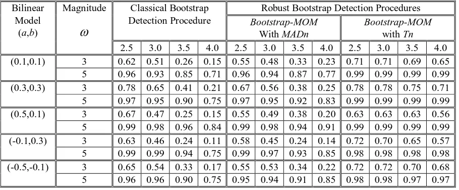
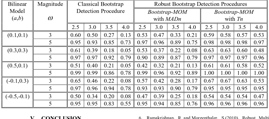
The performance of the robust bootstrap procedures on bilinear (1,0,1,1) model can be observed in Table 1 for detection of AO and in Table 2 for the IO detection. In both tables, the values in columns 3 through 14 represent relative frequency or proportion of correct detection of the respective type of outlier with correct location at t=40.
For both AO and IO, the results indicate that the performance of the outlier detection procedure of
bootstrap-MOMwithTn are better than bootstrap-MOMwith MADn. Meanwhile, the results for bootstrap-MOM with MADn and classical procedures are almost the same, but as the magnitude of outlier effect (
) and the critical value increase, the results of bootstrap-MOM with MADnprocedure have improved in comparison to the classical procedure. Based on the proportion of outlier correct detection, overall, the best result here is the procedure of bootstrap-MOMwith Tn. For a small critical value of 2.5 and 3.0, the results from bootstrap-MOM with Tn do not differ much from the other procedures but at larger critical value of 3.5 and 4.0, bootstrap-MOM with Tn clearly shows good results.
[image:5.595.72.527.531.719.2]The performance of proposed outlier detection procedures is better when larger
is used. In general, the proposed robust outlier detection procedures show good performance.Table. 1 The performance in detecting AO for bilinear (1, 0, 1, 1) model with critical values of 2.0, 2.5, 3.0 and 4.0 Bilinear
Model (a,b)
Magnitude
Classical Bootstrap Detection Procedure
Robust Bootstrap Detection Procedures
Bootstrap-MOM
With MADn
Bootstrap-MOM
with Tn
2.5 3.0 3.5 4.0 2.5 3.0 3.5 4.0 2.5 3.0 3.5 4.0 (0.1,0.1) 3 0.62 0.51 0.26 0.15 0.55 0.48 0.33 0.23 0.71 0.71 0.69 0.65
Table. 2 The performance in detecting IO for bilinear (1, 0, 1, 1) model with critical values of 2.0, 2.5, 3.0 and 4.0 Bilinear
Model (a,b)
Magnitude
Classical Bootstrap Detection Procedure
Robust Bootstrap Detection Procedures
Bootstrap-MOM
with MADn
Bootstrap-MOM
with Tn
2.5 3.0 3.5 4.0 2.5 3.0 3.5 4.0 2.5 3.0 3.5 4.0 (0.1,0.1) 3 0.60 0.50 0.27 0.13 0.53 0.47 0.33 0.21 0.59 0.58 0.57 0.53
5 0.95 0.93 0.85 0.73 0.97 0.96 0.89 0.75 0.98 0.98 0.98 0.97 (0.3,0.3) 3 0.61 0.39 0.18 0.05 0.53 0.37 0.22 0.08 0.63 0.63 0.60 0.48 5 0.97 0.97 0.92 0.79 0.90 0.89 0.87 0.79 0.97 0.97 0.97 0.96 (0.5,0.1) 3 0.51 0.40 0.21 0.05 0.42 0.32 0.21 0.13 0.61 0.61 0.58 0.52 5 0.99 0.99 0.86 0.78 0.99 0.96 0.92 0.89 1.00 1.00 1.00 1.00 (-0.1,0.3) 3 0.65 0.46 0.22 0.08 0.57 0.42 0.28 0.17 0.67 0.67 0.63 0.53 5 0.97 0.96 0.94 0.78 0.93 0.93 0.90 0.79 0.95 0.95 0.95 0.95 (-0.5,-0.1) 3 0.50 0.34 0.20 0.08 0.47 0.39 0.25 0.18 0.54 0.54 0.54 0.47 5 0.95 0.95 0.83 0.55 0.95 0.94 0.85 0.76 0.96 0.96 0.96 0.96
V. CONCLUSION
This paper proposed new robust outlier detection procedures for bilinear (1,0,1,1) model to detect AO and IO. Two robust estimators namely bootstrap-MOM with MADn
and bootstrap-MOM with Tn were introduced to improve the performance of classical bootstrap outlier detection procedure. Based on simulation results, the proportion of outlier correct detection using bootstrap-MOM with Tn
procedure is the best for all models and also for both types of outliers. The performance of detection for
bootstrap-MOM with MADn do not differ much from the classical procedure. However, the performance of bootstrap-MOM
with MADn procedure is better compared to the classical procedure, especially as the magnitude of outlier effect (
) and the critical value are increased. The robust bootstrap detection procedures are also better than classical bootstrap detection procedure, especially when the critical value is increased from 2.0 and 2.5 to 3.0 and 4.0.Generally, the proportion of correct detection is higher when the value of
increases. Overall, the proposed robust outlier detection procedures work well for all the bilinear (1,0,1,1) models used.ACKNOWLEDGEMENTS
This research work has been fully funded by the Research Acculturation Grant Scheme (RAGS: Code 12672) of the Ministry of Higher Education of Malaysia.
REFERENCES
1. Abuzaid, A.H.M.Mohamed, I.B. and Hussin, A.G. (2014). Procedures for Outlier Detection in Circular Time Series Models. Environmental and Ecological Statistics, 21, 793-809.
2. Efron, B. and Tibshirani, R., (1986). Bootstrap methods for standard errors, confident intervals and other measures of statistical accuracy.
Statistical Science1(1), 54-77.
3. Efron, B. and Tibshirani, R., (1993).An Introduction to the Bootstrap.
Journal of the American Statistical Association, 89, 428-436.
4. Hordo, M.Kiviste, A. Sims, A. and Lang, M. (2006). Outliers and/or Measurement Errors on the Permanent Sample Plot Data. In
Sustainable Forestry in Theory and Practice: Recent Advances in Inventory and Monitoring, Statistics and modelling, Information and Knowledge Management, and Policy Science.
5. Hristova, D. (2004). Maximum Likelihood Estimation of a Unit Root.
Studies in Nonlinear Dynamics & Econometrics, Vol 9, Issue 1, ISSN
6. Ramakrishnan, R. and Morgenthaler, S.(2010). Robust Multivariate and Nonlinear Time Series Models. Lausanne, EPFL. 10.5075/epfl-thesis-4688
7. Rousseeuw, P.J.and Croux, C.(1993). Alternatives to the median absolute deviation. Journal of the American Statistical Association.88, 1273-1283.
8. Shangodoyin, D.K. Ojo, J.K. Olaomi, J.O. andAdebile, A.O. (2012): Time Series Model for Prediting The Mean Death Rate of a Disease.
Statistics in Transition-new series, Vol. 13(2), 405-418.
9. Syed Yahaya, S.S. Othman, A.R. and Keselman, H.J.(2004). Testing the Equality of Location Parameters for Skewed Distributions Using
S1With High Breakdown Robust Scale Estimators. In M.Hubert, G.
Pison, A. Struyf and S. Van Aelst (Eds.), Theory and Applications of Recent Robust Methods,Series: Statistics for Industry and Technology, Birkhauser, Basel. 319 – 328.
10. Usoro, A.E. and Omekara, C.O. (2008). Bilinear Autoregressive Vector Models and their Application to Revenue Series. Asian Journal of Mathematics and Statistics1(1): 50-56.
11. Wilcox, R.R and Keselman, H.J. (2003). Repeated Measures ANOVA Based on a ModifiedOne-Step M-Estimator. Journal of British Mathematical and Statistical Psychology, 56(1): 15 – 26.