Imaging methods for understanding and improving visual training in the geosciences

(1)

Theses Thesis/Dissertation Collections

2-19-2013

Imaging methods for understanding and improving

visual training in the geosciences

Brandon May

Follow this and additional works at:http://scholarworks.rit.edu/theses

This Thesis is brought to you for free and open access by the Thesis/Dissertation Collections at RIT Scholar Works. It has been accepted for inclusion in Theses by an authorized administrator of RIT Scholar Works. For more information, please [email protected].

Recommended Citation

(2)

Improving Visual Training in the Geosciences

by

Brandon B. May

B.A. Mathematics & Physics Skidmore College, 

A thesis submied in partial fulﬁllment of the requirements for the degree of Master of Science

Chester F. Carlson Center for Imaging Science College of Science

Rochester Institute of Technology Rochester, New York

February , 

Brandon B. May Date

(3)

R, N Y

C  A

M.S. D T

T M.S.    B B. M             

    M.S.   I S

Dr. Nathan D. Cahill, esis Advisor Date

Dr. Jeﬀ B. Pelz, Commiee Member Date

(4)

(5)

is research project would not have been possible without the support of many people. I’d like

to thank my advisor Nate Cahill and the rest of my thesis commiee, Jeﬀ Pelz and Harvey Rhody, for their support and helpful suggestions in our weekly meetings as I discussed my progress and

developed my algorithms. anks also to Nate for providing valuable feedback on the initial dras of my thesis.

anks to Mitch Rosen for helping me to get started and involved with the GeoVis research project, and thanks for the efforts of Mitch, Jeff, John Tarduno, and Robbie Jacobs who first got

this project going.

For their great help while out imaging in the ﬁeld I’d like to thank Dave Kelbe and Tommy

Keane. Each of them proved invaluable in assisting me to capture many panoramas and keeping me entertained during the long drives through California. I’d also like to thank Karen Evans,

Piyush Agarwal, and Jason Babcock for their work capturing the eye-tracking data during the ﬁeld trips and for providing me with good company throughout our camping adventures. Karen

and Piyush also spent many hours with me in the CSI geing the projector system working well, for which I am very appreciative.

My ground truth analysis wouldn’t have been possible without the help of Tommy and a lot of manual clicking labor done by Sarah Piper, so thanks very much for that!

Finally, I’d like to thank my family for being supportive of my studies at RIT and always encouraging me to do my best.

RIT, February 

(6)

Experience in the ﬁeld is a critical educational component of every student studying geology.

However, it is typically diﬃcult to ensure that every student gets the necessary experience be-cause of monetary and scheduling limitations. us, we proposed to create a virtual ﬁeld trip

based off of an existing -day field trip to California taken as part of an undergraduate geology course at the University of Rochester. To assess the effectiveness of this approach, we also

pro-posed to analyze the learning and observation processes of both students and experts during the real and virtual ﬁeld trips.

At sites intended for inclusion in the virtual ﬁeld trip, we captured gigapixel resolution panora-mas by taking hundreds of images using custom built robotic imaging systems. We gathered data

to analyze the learning process by ﬁing each geology student and expert with a portable eye-tracking system that records a video of their eye movements and a video of the scene they are

ob-serving. An important component of analyzing the eye-tracking data requires mapping the gaze of each observer into a common reference frame. We have made progress towards developing a

soware tool that helps automate this procedure by using image feature tracking and registra-tion methods to map the scene video frames from each eye-tracker onto a reference panorama

for each site.

For the purpose of creating a virtual ﬁeld trip, we have a large scale semi-immersive display

system that consists of four tiled projectors, which have been colorimetrically and photomet-rically calibrated, and a curved widescreen display surface. We use this system to present the

previously captured panoramas, which simulates the experience of visiting the sites in person. In terms of broader geology education and outreach, we have created an interactive website that

(7)

5 Virtual Field Trip

40 5.1 Semi-immersive Virtual Environment . . . 40

5.1.1 Multi-projector Calibration . . . 40

5.1.1.1 Geometric Registration . . . 41

5.1.1.2 Photometric and Colorimetric Calibration . . . 44

5.1.2 Rendering Images for Display . . . 45

5.1.3 Projector Tiling Solution. . . 46

5.2 Online Virtual Field Trip Interface . . . 47

5.2.1 Google Earth . . . 47

5.2.2 Site Pages . . . 48

5.2.3 Panorama Gallery . . . 49

6 Conclusions

52 6.1 Future Work . . . 53

Appendix A Software

55

(9)

List of Figures

. Students wearing the mobile eye-tracking system. . . 5

. Example visualization of SIFT features detected in an image. . . 8

. Example of image registration using SIFT and RANSAC with a homography model. 12 . Olympus camera electronic shuer release cable wiring diagram. . . 15

. GigaPan unit with support bracket aached. . . 16

. Extended camera mounting plate. . . 16

. Portable D-cell baery pack for the GigaPan. . . 17

. Second generation robotic imaging system. . . 20

. Optimized panorama shooting paern. . . 21

. Typical results from a successful panorama capture. is particular example is of Ubehebe Crater in California. . . 22

. Wide-baseline stereo capture of Monte Bello Ridge in California. Notice the tripod in the distance on the le and in the foreground on the right. . . 22

. A sample video frame from the eye-tracker scene camera, overlaid with the eye camera and gaze data. . . 24

. Equirectangular (spherical) rendering of the panorama taken at the Ubehebe Crater in California. e black areas represent portions of the sphere where image data was not captured. . . 28

. Spherical to Cylindrical Panorama Projection Diagram . . . 29

. Spherical to Planar Panorama Projection Diagram . . . 30

(10)

. A visualization of a frame of the scene video mapped onto the panorama via its

homography. . . 35

. e nine control points selected for use in the ground truth evaluation of the scene at Inspiration Point, Yosemite National Park, California. . . 36

. e geometric projection error in pixels on the panorama, computed from the man-ual points selected in each video frame corresponding to each of the nine control points. . . 36

. Plot of the mapped video points for each of the nine control points. . . 37

. Close-up views of the mapped video points for each of the nine control points. . . . 38

. Box plots of the statistical distribution of geometric projection errors corresponding to each of the nine control points. . . 39

. Flow chart describing the projector calibration algorithm. . . 41

. Typical arrangement of projectors, camera, and cylindrical projection surface. . . . 42

. e light paern used to geometrically calibrate the projectors and display wall. . . 42

. Cylindrical surface and world coordinate system. . . 43

. Local coordinate system for projector calibration. . . 44

. ree stages of projector calibration. . . 46

. Example of a tiled version of the panorama taken at Inspiration Point. . . 47

. A screenshot of the online virtual ﬁeld trip interface. . . 48

. A pop-up is presented with additional information when a placemark icon is clicked. 49 . A screenshot of the site page for Inspiration Point. . . 50

. A screenshot of the panorama gallery; an alternative to the Google Earth view. . . 50

(11)

Introduction

Experience in the ﬁeld is a critical educational component of every student studying geology.

However, it is typically diﬃcult to ensure that every student gets the necessary experience be-cause of monetary and scheduling limitations. If anything, the ﬁeld trip will be restricted to a

single-day with a small group of people. Perhaps in these cases it would be effective to bring the field experience to the students instead of sending the students out into the field. us, we

proposed to create a virtual field trip based off of an existing -day field trip to California taken

as part of an undergraduate geology course at the University of Rochester []. During the ten-day

ﬁeld trip both geology students and expert geologists visit a number of geologic sites.

In order to create a virtual ﬁeld trip that realistically simulates ﬁeld experience, the

origi-nal sites must be carefully captured in such a way that later allows for a realistic simulation. erefore, at sites intended for inclusion in the virtual ﬁeld trip, we captured gigapixel

resolu-tion panoramas by taking hundreds of images using custom built robotic imaging systems. e individual images were processed and stitched together at a later time to form high-resolution

panoramic images. To create the virtual ﬁeld trip the panoramas are then projected for observa-tion in a semi-immersive display system.

An important part of this project is the ability to analyze the learning process during the real experience as compared to the virtual one as well as the educational eﬀectiveness of each.

(12)

learning based on where they look. When both in the ﬁeld and using the semi-immersive display,

each geology student is ﬁt with a portable eye-tracking system that records a video of their eye movements and a video of the scene they are observing. Aerwards, these data can be processed

to determine where the person was looking (their gaze) and for how long. To provide a baseline for comparison, several expert geologists were present during the real and virtual ﬁeld trips to

participate in the same experience as the students.

It is possible to compare the eye-tracking information from one observer to the next and from

the same observer to themselves over a period of time to evaluate information such as novice-expert diﬀerences, the learning process through time, and diﬀerences in the learning experience

between the real and virtual ﬁeld trips. e ability to make these comparisons relies on having a common reference frame on which to compare the gaze data. Typically ﬁxations are ploed

manually from each observers scene video onto a panorama of the scene, however this is a time consuming process. We have made progress towards developing a soware tool that helps

auto-mate this procedure by using video feature tracking and image registration methods to map gaze information from each video frame onto a reference panorama.

In terms of geology education and outreach, the panoramic images collected for the virtual ﬁeld trip could be incorporated into a range of geoscience courses at every educational level. e

database of images could even prove useful to researchers in the ﬁeld of computer vision for test-ing feature detection, image stitchtest-ing, structure from motion, and other techniques. Cognitive

science educators and researchers could also ﬁnd value in the large database of video eye-tracking data of novices and experts viewing geological landscapes. Towards these goals, we have created

an interactive website that uses Google Earth as the interface for visually exploring the

panora-mas captured for each site []. It has the potential to incorporate additional data such as audio

recordings, eye-tracking data, and other information relevant for use as an educational tool. e rest of this thesis is focused on presenting the details of our work. In chapter  we present

an overview of the prior work related to this research. We describe the tools and techniques for capturing gigapixel resolution panoramas out in the ﬁeld in chapter . In chapter  we describe the

(13)

environment and describe the online virtual ﬁeld trip interface. We conclude and propose possible

directions for future work in chapter .

Novel contributions are presented in each of the chapters three through ﬁve. e following

summarizes these contributions according to each chapter:

Ch. : Imaging in the Field

• Built a portable gigapixel resolution robotic imaging system using a telescope mount, DSLR camera, baery pack, and wireless bluetooth control via tablet computer.

• Designed an eﬃcient shooting paern on the sphere to minimize time of capture.

Ch. : Image Processing

• Developed a two-pass SIFT feature tracking algorithm for videos.

• Developed a feature matching algorithm that used a multiple level-per-octave SIFT ap-proach to be robust to very large diﬀerences in resolution and scale.

• Developed a video keyframe selection algorithm based on initial video frame to panorama homography computations.

• Developed a method to match video frames to a reference panorama by calculating a ho-mography by combining information from SIFT video tracking, multi-level feature

match-ing, and keyframe selection.

Ch. : Virtual Field Trip

• Created a semi-immersive virtual ﬁeld trip by geometrically, photometrically, and colori-metrically calibrating a high-resolution multi-projector display system.

(14)

Related Work

is research covers a variety of topics and in what follows we provide a general overview of

the related work. First we discuss mobile eye-tracking and the portable systems we used in the ﬁeld. Next we present a review of image feature detection and matching and how it can be

used to track features through a video sequence. We then discuss how image registration can be computed with these detected features using a speciﬁc image transformation model. Finally, we

review techniques for calibrating multiple projector display systems.

2.1 Mobile Eye-tracking

e ﬁrst eye-tracking systems were created in the s and were based on mechanical devices

that recorded eye movements by aaching a device directly to the observer’s eye. A much less invasive technique was developed around  which used photographic technology to record

eye movements by taking pictures of the reﬂection of a light source directed towards the eye, and this is at its essence the same technique used in our mobile eye-tracking systems, albeit less

sophisticated. ere have been many eye-tracking systems designed based on this technique, most of which require the user to stay relatively still, and certainly not be walking around. Some

examples are the lens and mirror systems used by Yarbus, electromagnetic coil systems,

(15)

In order to take eye-tracking out into the ﬁeld, we use a portable and robust system designed

by Jason Babcock of Positive Science, who designed the ﬁrst mobile prototype in  while here

at the Multidisciplinary Vision Research Laboratory (MVRL) [, ]. is system uses the pupil

and corneal reﬂection method to track the eye of the person wearing it. e motion of the eye and a video of the scene are recorded using a piece of headgear that the observer wears. e

base of this headgear is the lightweight frame of a pair of glasses with the lenses removed. It has mounted on it a small video camera that records what the observer is seeing and another small

infrared camera mounted below the eye, illuminated by an infrared LED, that records and image of the eye and its reﬂections. e system is designed to be worn as a backpack that contains a

[image:15.612.161.451.313.509.2]

laptop and various pieces of electronics that interface with the headgear (Figure.).

Figure .: Students wearing the mobile eye-tracking system.

e pupil and corneal reﬂection method used by this eye-tracking system works in the fol-lowing manner. e infrared LED mounted next to the eye camera on the headgear provides

il-lumination of the eye as well as a singular specular reflection off of the cornea, called the corneal reflection (also known as glint or the first Purkinje reflection). To estimate the gaze of the

ob-server the center of the dark pupil and the center of the corneal reﬂection must ﬁrst be determined by some feature detection algorithm. As the eye moves, the relative location of the corneal

reﬂec-tion to the pupil center changes systematically and can thus be used to calculate gaze based on

(16)

the reﬂections of infrared light from the scene oﬀ the eye, which can make pupil and corneal

reﬂection detection diﬃcult.

e system must be calibrated before use to be able to determine what the

pupil-to-corneal-reﬂection relationship is for accurate eye-tracking. is calibration is typically done by having the observer ﬁxate one at a time on a set of known points in the scene. A transformation model

can then be computed from this data that allows the relative distance measurement to be mapped to a gaze location on the scene video. In the ﬁeld each observer wore a hat to help prevent

sunlight from ﬂooding the eye. Each time the eye-tracking system was worn, it was calibrated by having the observer ﬁxate on a single point while moving their head through a ‘+’ and ‘x’

paern, pausing their motion several times in each segment. is procedure created the set of data points necessary for calibration the relative pupil-to-corneal-reﬂection distance to real gaze

information. It is this gaze information that gets mapped to the panorama via the scene video in the registration algorithm of Ch. .

2.2 Image Feature Detection and Matching

Image feature detection is the foundation for many algorithms that rely on the knowledge of anchor points whose locations are both stable and accurate, such as camera calibration, pose

estimation, D reconstruction [], object tracking, and image registration [–]. An important

example of local features are interest points (keypoints), which can be described by analyzing

the appearance of regions of pixels surrounding an particular point location. Another possibility is to use edge information that can be described by local appearance and orientation, or linked

together to form paerns of lines and curves. It is desirable in the case of matching images to have a feature detector that is robust to both geometric image transformations such as rotation,

scale, and viewpoint, as well as image noise [–]. To be robust to these transformations means

that the same feature can be reliably detected in an image both before and aer going through

these changes. is robustness makes it possible to match images that have similar content but were taken under diﬀerent conditions (such as location, time, orientation, and hardware).

(17)

in Ch. , we use a local keypoint feature detector called SIFT, which stands for Scale Invariant

Feature Transform []. In particular, we use the version packaged with the VLFeat toolbox for

MATLAB [,]. e SIFT feature detection algorithm detects and converts regions of interest

into an invariant descriptor representation that can be used to ﬁnd matches with other descrip-tors. For robustness, it looks for features that are stable over multiple resolution scales of the

image []. It uses a Gaussian function to create a multi-level image pyramid over each octave of

the original image. It then subtracts these levels to make a set of Diﬀerence of Gaussian (DoG)

images.

SIFT detects candidate features as extrema by comparing a pixel to the set of its  neighbors

in the current level ( neighbors), next upper level ( neighbors), and previous lower level ( neighbors). Once this feature is identiﬁed, the gradient at each pixel in a x region around the

feature at the appropriate level is computed, weighted by the distance from the feature by another Gaussian function. is weighting helps to reduce the eﬀect of gradients far from the center.

Looking at the histogram of gradients, the peak is assigned as the dominant orientation. Next, this region is divided into x areas combining the gradients into an -bin histogram (relative to

the dominant orientation) for each area. Computing the gradients this way is what makes the feature invariant to rotation. ese  numbers form the raw descriptor of the feature keypoint.

is set of numbers is saved as a normalized vector, subject to a maximum component value of

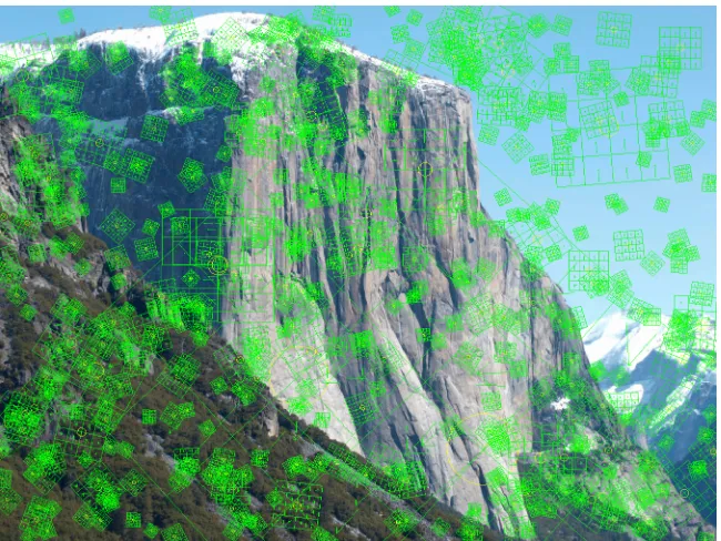
.. If any of the components are clipped, the vector is renormalized to unit length. Figure.

shows an image with a representation of its SIFT features ploed. e size of each grid represents the scale at which the feature was found, and its orientation represents the dominant gradient

at that location. e arrows within each subregion represent the dominant orientation of that section of the image [].

To determine how well particular SIFT feature descriptors match one another, the diﬀerence between the two -element vectors is measured with a Euclidean norm. When a single

descrip-tor is being matched to a set of other descripdescrip-tors, a match is deﬁned as the nearest neighbor in the Euclidean sense, subject to the constraint that the ratio of the distance between the descriptor

(18)

[image:18.612.145.470.72.316.2]

Figure .: Example visualization of SIFT features detected in an image.

2.3 Image Registration Using Homographies

Image registration using local features ﬁnds applications ranging from panography and pose es-timation to structure from motion and augmented reality. It is also used when creating high

resolution maps by aligning and stitching together satellite imagery. When performing image registration, once the features have been detected in multiple images, a pairwise matching

algo-rithm can be run to determine a hypothetical set of feature matches between them. is initial set of feature matches is called the putative set because it remains to be determined which are

true matches and which are false positives. If a geometric transformation model is available, the matches can be ﬁt to this model and kept only if they match the transformation suﬃciently well.

is can be done by selecting a small sample set to compute the transformation based on the model, then expanding that test to include the rest of the matches. is process can be repeated

a number of times until a suﬃciently close transformation restricted to the particular model is found, or stopped aer a number of iterations if not. e process of testing a small sample and

using it to verify the larger dataset is called random sample consensus (RANSAC) [].

(19)

most part the panoramas we capture are of distant scenes so that the relationship between the

panorama and a frame of video from the scene camera on the eye-tracker is just a pure rota-tion. is essentially means that the scene content we wish to match between the panorama and

the video is so far away, that the change in translational position between where the panorama was captured and where the video was captured introduced a negligible amount of parallax for

that region. e homography,𝑯, is an eight parameter matrix transformation model that allows

matching two images with a change in position, rotation, skew, and perspective. In general, the

homography transformation with point correspondances𝒙_𝑖 ↔ 𝒙_𝑖may be wrien as,

𝒙_𝑖 = 𝑯𝒙_𝑖. (.)

To enable a linear solution for𝑯, this equation can be rewrien in a form that makes use of the

cross product,

𝒙_𝑖 × 𝒙_𝑖 = 0 = 𝒙_𝑖× 𝑯𝒙_𝑖. (.)

If𝒙_𝑖 = (𝑥_𝑖, 𝑦_𝑖, 𝑤_𝑖)⊤ _{and the j-th row of the matrix}_𝑯 _{is denoted by}_𝒉𝑗_{, this may be rewrien as,}

⎡ ⎢ ⎢ ⎣

𝟎⊤ −𝑤_𝑖𝒙⊤_𝑖 𝑦_𝑖𝒙⊤_𝑖

𝑤_𝑖𝒙⊤

𝑖 𝟎⊤ −𝑥𝑖𝒙⊤𝑖 ⎤ ⎥ ⎥ ⎦ ⎡ ⎢ ⎢ ⎢ ⎢ ⎣ 𝒉1⊤ 𝒉2⊤ 𝒉3⊤ ⎤ ⎥ ⎥ ⎥ ⎥ ⎦

= 0 = 𝑨_𝑖𝒉. (.)

Since each point correspondence yields two independent equations, at least four point

correspon-dences are necessary to ﬁnd a solution for𝒉. For𝑛matches, stack the individual𝑨_𝑖matrices into

a single matrix𝑨. To solve for𝒉, take the singular value decomposition of𝑨,

𝑨 = 𝑼𝑫𝑽⊤. (.)

e unit singular vector corresponding to the smallest singular value is the solution. If 𝑫 is

diagonal with positive entries arranged in descending order, then𝒉is the last column of𝑽. is

(20)

given a set of putative matches, it is necessary to perform ﬁltration using RANSAC before trying

to compute a valid homography.

RANSAC works by selecting a random sample of descriptor matches to compute an initial

estimate for the particular model being used, in this case a homography, 𝑯. Using this model,

residuals are computed for all of the feature matches by computing the diﬀerence in the measured

and mapped points:

𝑟_𝑖= 𝒙_𝑖 − ̂𝒙_𝑖 (.)

𝒙_𝑖 = 𝑯𝒙_𝑖 (.)

where𝑟_𝑖is the residual,𝒙_𝑖 are the locations mapped using the homography, and𝒙_𝑖̂ are the

mea-sured locations from the feature points. It then counts the number of inliers that are within a

few pixels of their predicted location. is process repeats a for a certain number of trials

un-til returning the sample set that yields the model with the largest number of inliers. Figure.

shows an example of the result of image registration using SIFT feature descriptors and RANSAC with homography model. Before running RANSAC the putative match set has a large number of

outliers. Aerwards, a group of inliers is successfully selected and an accurate homography is computed.

2.4 Projector Calibration

In general, when registering multiple projectors on a non-planar surface, multiple cameras are

needed in order to reconstruct the D surface of the display. In [] they use a stereo camera

rig to reconstruct non-planar quadric surfaces using such techniques as conformal mapping and

quadric transfer to minimize distortion aer the geometric registration. Another method, [],

ﬁrst achieves camera and projector calibration through D ﬁducials and then reconstructs the sur-face of the display by using many structured-light paerns. ere are other registration methods

that make use of only one camera for non-planar surfaces, however these are typically

(21)

the camera and avoids reconstructing the display geometry entirely.

Intra-projector variation, inter-projector variation, and overlap variation are the three main categories of spatial color changes in multiple projector displays. Most existing blending

meth-ods don’t address all of these issues and thus have suboptimal solutions. One of these methmeth-ods,

[], proposes a gamut matching method for tiled display walls, however gamut matching

sig-niﬁcantly degrades the color quality of the display by restricting the common achievable gamut

[]. Another method, [], matches the luminance transfer functions to achieve a luminance

balancing without considering the projector chrominance variations.

In [], they present a technique to calibrate multiple casually aligned projectors on a

cylin-drical surface using a single camera, where the cylinder is a vertically extruded surface and the aspect ratio of the rectangle formed by the corners of the screen is known. ey achieve

ac-curate geometric calibration of multiple projectors on a cylindrical display without performing

an extensive stereo reconstruction. Our method, based on [], is likewise able to recreate the

D surface of the display using a single camera without needing to restrict the ﬁnal viewpoint to

that of the cameras position. e constrained gamut morphing algorithm created by [] removes

variations due to diﬀerences in chromaticity gamuts across the projectors, the vigneing eﬀect of each projector, and the overlap across adjacent projectors. ey demonstrate color seamlessness

across multiple projectors for both planar and curved displays.

Basing our approaches on [], the colorimeteric & photometric calibration steps we

imple-mented consider both spatial variations in luminance within the projectors and diﬀerences in

chromaticity between the projectors. By combining techniques from [] and [], we created a

(22)

(a) Scene video frame (b) Photo of El Capitan

(c) Putative SIFT feature matches (d) Filtered SIFT feature inliers

[image:22.612.82.539.123.424.2]

(e) Video frame registered to photo of El Capitan

(23)

Imaging in the Field

One of the main imaging goals during the ﬁeld trip is to be able to capture a detailed visual

rep-resentation of each important geologic site. is serves several purposes, of which an important one is being able to recreate the experience as accurately as possible within a virtual environment,

while another is to use this data to aid in the eye-tracking analysis. It would also be useful to the geology education community to be able to utilize the data in a practical way for pedagogical

purposes. Deciding on what type of imaging system to use depends both on these desired results as well as the practicality of using the system while in the ﬁeld.

It is necessarily the case that being on the ﬁeld trip involves driving (and sometime walking) to remote locations that don’t have a readily available power source, visiting a potentially high

number of locations during the period of a day, and facing a wide range of weather conditions over the entire trip. us, the imaging system must be portable and have its own power source, and

because of the number of sites visited each day it must also assemble, function, and disassemble quickly and easily. e components that make up the system also need to operate well in both

hot and cold temperatures and be somewhat resistant to moisture and dust.

A simple imaging system that seems to satisfy the above conditions is to use a high resolution

Digital Single Lens Reﬂex (DSLR) camera mounted on a tripod to take an image of each site. However, the ﬁeld of view for a camera with a typical lens that has a full-frame equivalent focal

(24)

elements usually cover a larger ﬁeld of view it would be necessary to take multiple images to

cover them. If the images were taken by rotating the camera on the tripod head they could be processed into a large panoramic image of the scene. It turns out that there are robotic systems

for automating this image taking procedure which can yield enough data to create panoramas of up to several gigapixels in resolution.

3.1 Robotic Imaging Systems

3.1.1 Gigapan

e ﬁrst robotic imaging system built for panoramic imaging on the ﬁeld trip was based on the GigaPan EPIC  designed by researchers at Carnegie Mellon University in collaboration with

NASA Ames Intelligent Systems Division’s robotics group []. e GigaPan unit itself can be

easily mounted on a tripod and consists mainly of a camera mounting bracket, two stepper motors

run by a micro-controller and the built in soware, a servo motor to physically press the camera’s shuer buon, and a six AA baery power supply brick. e camera chosen to be used with the

GigaPan was an Olympus E- DSLR with an - mm zoom lens and a  megapixel CCD sensor. e two stepper motors control the horizontal and vertical rotations of the camera calculated by

the soware for the images needed to capture the panorama. e stock conﬁguration of the GigaPan, however, needs a few modiﬁcations to make it more robust before it is ready to be used

in the ﬁeld.

3.1.1.1 Modifications

Instead of using the built in servo to press the camera’s shuer buon it would be more eﬀective to trigger a remote shuer release via a cable plugged into the camera. Otherwise the servo

tends to shake the camera while taking a picture, it draws an unnecessary amount of power, and it physically limits the placement of the camera. e EPIC  has a seing to enable an electronic

(25)

empty remote port of the GigaPan to the camera.

is cable must be built and wired speciﬁcally for the model of camera being used to comply with the required shuer release signal. For example when using a Hitec Servo cable to interface

with the GigaPan remote port in conjunction with an Olympus camera multi connector to inter-face with the camera, the Olympus camera multi connector requires that both the “shuer full

press” (white) and “shuer half press” (yellow) wires be connected to the yellow Hitec wire and

the “shuer ground” (red) must be connected to the black Hitec wire (Figure.). With this

con-Figure .: Olympus camera electronic shuer release cable wiring diagram.

ﬁguration, the camera shuer will ﬁre automatically when the signal is sent through the remote

port without having any mechanical interactions.

e stock conﬁguration also has some problems with handling heavier cameras like a DSLR

with a relatively heavy lens aached. One reason is because all of the weight is supported on one side of the unit where the camera mounting bracket is aached to the motor while the other

side of the bracket is le ﬂoating freely. Another is that the center of mass of the camera isn’t centered on the rotational axis of the vertical servo motor which causes the motor to work harder

to rotate the camera. To remedy this issue a support bracket was custom installed onto the side of

the unit to support the camera mounting bracket (Figure.). e slots on the camera mounting

plate were also extended so that the camera could be mounted further back to be able balance the camera about the vertical rotation axis so that very lile torque is required to rotate it up and

down (Figure.).

(26)

[image:26.612.236.375.288.386.2]

(a) Front view. (b) Side view.

Figure .: GigaPan unit with support bracket aached.

Figure .: Extended camera mounting plate.

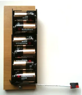
powering the GigaPan through shooting hundreds of images without having to replace the

bat-teries too oen. A baery pack that used D baeries was built for this purpose (Figure.). Since

it was too large to be aached to the GigaPan itself, it was mounted to the leg of the tripod and

power was routed to the unit through a  meter long power cable terminated with “Anderson Powerpole” connectors to facilitate connecting and disconnecting the baery pack. e length

of the power cable allows the GigaPan the freedom to make360⋅_{rotations without geing tangled}

in the tripod. With this power supply the GigaPan can be used for long periods of time without

(27)

[image:27.612.235.379.73.240.2]

Figure .: Portable D-cell baery pack for the GigaPan.

3.1.1.2 Panorama Capture Setup

To prepare the imaging system to capture a panorama requires assembling the components, set-ting the appropriate camera parameters, and conﬁguring the GigaPan soware. First, the camera

is aached to the mounting bracket of the GigaPan and the remote shuer trigger cable is plugged in (aer making sure the baery pack is charged and enough space is le on internal storage to

hold the images for the panorama). en the GigaPan is clipped into the tripod head at which point the baery pack can be plugged into it. is system is carried to the desired location for the

point of view of the panorama, which is usually close to where the students viewing the scene will be standing. Once the tripod is setup and level, the camera parameters can be conﬁgured.

e camera should have a ﬁxed focus, focal length, white balance and exposure throughout the entire image acquisition process to produce images that will blend together well to form the

ﬁnal panorama. e aperture should be set small enough to have a large depth of ﬁeld so that both distant features and close foreground appear in focus; in practice it was set to around f/.

For a consistent and easy to set focal length the lens was set to its maximum value of  mm. is level of zoom allows for detailed visual information to be captured and generation of

high-resolution panoramas. Now the GigaPan soware needs to be given instructions on what type of panorama is desired so it can compute and execute the appropriate shooting sequence.

(28)

aer moving the camera to the next position for it to stabilize and signal it to take another. e

GigaPan soware calculates the ﬁeld of view by having the user position the camera at two positions diﬀering only by vertical rotation. e scene content at the top of the second position

must overlap slightly with the scene content that was present at the boom of the ﬁrst position for an accurate estimate. Aer the ﬁeld of view is set, it doesn’t need to change when using the

same camera and lens setup for each panorama. For the purposes of imaging in the ﬁeld, the scenes were always bright enough to have a fast enough shuer speed so that the other delays

could be set to their minimum values.

Aer the initial setup, the panorama is taken using one of two methods. e ﬁrst method is

to set the boundaries on the panorama by telling the soware where the upper le and lower

right corners should be. e second method is to tell the soware to take a360⋅ panorama and

deﬁne the top and boom of the vertical extent of the panorama. e shooting paern necessary for taking the panorama is then calculated and executed.

3.1.1.3 Shooting Pattern

e shooting paern is deﬁned by a rectangular grid with a certain number of rows and columns to zig zag through to take the images. e number of columns is ﬁxed for all rows based on the

amount needed to image at the horizon position with a minimum of % overlap between the images. is shooting paern can be rather ineﬃcient because, for example, when the camera is

pointing in a direction above or below the horizon the amount of images needed is fewer than the amount at the horizon. is can lead to situations where the camera will be imaging the zenith

position many times over (equivalent to the number of columns) when in reality only one image is needed. ough the shooting paern is simple, it requires extra time to complete that wouldn’t

otherwise be needed. It was decided that for the following years ﬁeld trip a new robotic system would be used that allowed more control over this aspect of the panorama imaging process in

(29)

3.1.2 Panogear

e next generation robotic imaging system was built based oﬀ of a design of the motorized

panoramic head called “Panogear” by Kolor []. We used a “Merlin-Orion TeleTrack GoTo”

al-tazimuth telescope mount aached to a tripod for the main body of the system. e original

purpose of this mount is to allow ﬁne-controlled motorized tracking of celestial objects with a small telescope, however this basic functionality can be taken advantage of to provide precise

control over the orientation of a camera instead. e device comes with an “Orion GoTo” com-puterized hand controller, a telescope mounting bracket, and a  volt power supply. For our

purposes, a bluetooth dongle was purchased to replace the hand controller. is dongle plugs into the data port on the Merlin and wirelessly communicates with a computer running control

soware called “Papywizard” []. is soware is designed for taking panoramas with the

Mer-lin and is able to instruct it to point in a particular direction and trigger the camera to take an

image. e physical trigger is sent via a cable connected from the “snap” port on the Merlin to the cameras control port. For this system the camera was upgraded to an Olympus E-PL DSLR

with a -mm zoom lens fied with an ultraviolet filter. ough it was custom built, a couple modifications were still necessary to make it more suitable for our needs.

3.1.2.1 Modifications

A metal mounting plate for the camera was fabricated in order to be able to aach the camera

to the Merlin at a vertical orientation and in such way that the principal point of the lens is centered on the horizontal and vertical rotation axes. Doing so eliminates nearly all parallax

eﬀects between photos taken while pointing at diﬀerent locations in the scene and makes it easier to create an accurate panorama from the constituent photos. Additionally, as was done with the

Gigapan, an external D-cell baery pack was built and aached to the leg of the tripod. is power supply allowed the unit to be portable and was able to operate the Merlin throughout the

(30)

3.1.2.2 Panorama Capture Setup

is system requires a quick setup before its ready to take a panorama. Assuming the Merlin has

been mounted to the tripod, the camera mounted to the Merlin with the snap cable connected, and the power switched on, the ﬁrst thing to do is to make the connection to the bluetooth

hardware dongle from the computer running the Papywizard soware. Once the connection has been established, like with the Gigapan, the camera must have set a ﬁxed focus, focal length,

white balance, and exposure. For ease of use and consistency a focal length of mm for the lens was used. To take the panorama a predeﬁned shooting sequence (discussed below) is selected in

the Papywizard soware and the panorama capture is started. During the sequence the camera captured both RAW and JPEG images. e JPEG images can be used for faster processing in the

subsequent panorama stitching procedure, while the RAW images capture -bit data and may

be used to perform nondestructive adjustments of the photos. Figure.shows a typical setup of

[image:30.612.234.378.384.679.2]

this robotic system.

(31)

3.1.2.3 Shooting Pattern

To capture the panorama, a sequence of overlapping images was taken by instructing the

tele-scope mount to follow a shooting paern speciﬁed to cover a spherical view of scene. e Papy-wizard soware will read in an XML ﬁle specifying the order of shooting based on pitch and yaw

angles. We developed an XML generator that creates this ﬁle using parameters such as the cam-era focal length and desired percentage overlap of images as input. e speciﬁc shooting paern

is designed to take advantage of the spherical geometry of the image capture. If a standard grid paern is selected, an excessive amount of images are taken at any vertical angle other than the

horizon. For example, if the camera is pointing away from the horizon its ﬁeld of view captures a greater portion of the scene relative to the horizontal rotation axis than it does when level. us,

we designed our paern so that the minimum number of images was taken to guarantee coverage

and ensure the appropriate amount of image overlap (Figure.).

Figure .: Optimized panorama shooting paern.

e shooting paern is also speciﬁcally designed to shoot entire rows at a time alternating

about the horizon. For example, the horizon row would be captured ﬁrst, then the row below the horizon, then the row above the horizon, and so on alternating back and forth until either

(32)

imagery. In this way the sites were captured more quickly and eﬃciently and less prone to error

due to technical glitches in the hardware or soware. e ﬁnal set of images usually looks similar

[image:32.612.89.523.161.276.2]

to what is shown in Figure..

Figure .: Typical results from a successful panorama capture. is particular example is of Ubehebe Crater in California.

3.1.3 Stereo Imaging

Typically, multiple panoramas of the same scene were captured simultaneously using two

identi-cal robotic systems placed a wide distance apart (Figure.). e distance was measured each time

Figure .: Wide-baseline stereo capture of Monte Bello Ridge in California. Notice the tripod in the distance on the le and in the foreground on the right.

[image:32.612.161.451.437.632.2]

(33)

case one of the devices malfunctioned and prevented capture of a scene. Secondly, it provides an

option to choose which panorama is best suited for presentation in the virtual environment and that has best captured all of the features of geologic importance. On this note, one of the tripods

was placed very close to the perspective that the students would have while viewing the scene. is makes the task of mapping gaze data to the panoramas easier as well. Finally, it opens up

the possibility of generating some sparse D geometry about the scene from the widely separated pairs of images.

3.2 Imaging Augmented with GPS

Two identical hand-held Garmin GPS units, an “active” unit and a “base” unit, were used to mea-sure various pieces of location information particularly useful for the ﬁeld trip. e base unit was

run continuously throughout the day in the vehicle taking a measurement every second to keep a record of where we went, when, and for how long. To increase the chances of an accurate signal

an external antenna was mounted to the roof of the vehicle and routed in through the driver side door to connect to the hand-held unit. Digital markers were set every time we arrived and le a

stop to make it easier to analyze the location information aerwards.

To augment our panoramas with ground truth location data, the active unit was used to keep

track of the position of each tripod as it was placed in the ﬁeld at each site. is also provided a second measurement of the distance between tripods when stereo panoramas were being

cap-tured. e active unit was carried around at the site while taking individual photos of the imaging setup and scene to provide more reference frames for analyzing the geometry of the scene. e

times on the cameras were manually synchronized to the GPS time so that the locations of the photographs could be determined aerwards without having to manually mark them.

Because the GPS measurements have some error associated with them it would be desired to have a way to reduce the error by combining the measurements from the active and base units. By

calculating the ﬂuctuations away from average in the base unit might be possible to compensate for any location data ﬂuctuations in the active unit, yielding more accurate location information

(34)

3.3 Scene Video from Eye-trackers

In addition to the high-resolution image capture systems, there were video cameras aached to

the headgear of every eye-tracker to capture a view of what each person was observing. ey are typically used for calibrating and visualizing the gaze of each individual observer onto the

video of the scene (Figure.), but also provide another source of content that may eventually

[image:34.612.163.450.239.455.2]

be incorporated into the virtual ﬁeld trip. e fact that there are a large number of scene videos

Figure .: A sample video frame from the eye-tracker scene camera, overlaid with the eye camera and gaze data.

from slightly diﬀerent viewpoints provides interesting possibilities for tracking the pose of each

observer and simultaneously visualizing the gaze of each observer in a common D reference frame. e scene videos are low resolution and have poor color ﬁdelity, but have a wider than

typical ﬁeld of view because of the use of a wide-angle lens. Unfortunately, because of this lens, there is a some amount of lens distortion present in the video which should be compensated

for before doing any image analysis. One way of doing this is to image a known object, like a checkerboard, and calculate the radial distortion model necessary to straighten out all of the

curved lines []. Due to the nature of the wide dynamic range that comes from being outdoors

(35)

perform comparisons between the video content and the ultra high ﬁdelity panoramas. A portion

of the next chapter discusses a method for mapping observer gaze onto the panorama using their video as a guide despite this diﬃculty; a step towards realizing the goal of a common reference

(36)

Image Processing

4.1 Panorama Generation

Generating the high-resolution panoramas requires an image stitching and blending procedure

to combine all of the individual photographs from a particular capture into a uniﬁed representa-tion of the scene. Many soware packages are available for this procedure, but we have found

the Autopano Giga program by Kolor to be the fastest and most reliable for our needs []. is

soware detects and builds panoramas from an arbitrary set of input images. It uses SIFT feature

detection and matching to ﬁt a similarity or homography image transformation model in con-junction with outlier rejection to generate the ﬁnal image feature correspondences. If desired,

there is an option to simultaneously correct for any lens distortions that may be present in the images.

e Autopano Giga soware also has the ability to take into account the particular shooting paern used with either the GigaPan robot or PapyWizard soware when making its calculations.

For images taken with the GigaPan one may select the shooting paern that corresponds with what was setup in the GigaPan soware. For images taken using the Papywizard soware, the

XML ﬁle that speciﬁes the shooting paern can be selected. In both cases a small preview is

(37)

these import options typically produces a more accurately stitched panorama. Once this stitching

step is completed, the panorama is visualized using one of several projection methods prior to the ﬁnal rendering.

4.1.1 Projection Methods

When visualizing a spherically captured panorama, it is typical to use some projection method to represent the entire scene on a two dimensional image plane – analogous to creating a map of the

earth. Autopano Giga has several projection options, namely spherical, cylindrical, and planar. Also known as equirectangular projection, spherical projection is simply an angular

parameter-ization of the panorama. In a panoramaℎpixels tall and𝑤pixels wide, the𝑥and𝑦coordinates

are related to the longitude,𝜃, and the latitude,𝜙, by,

𝑥 = 𝑤

2 1 + 𝜃 𝜋

𝑦 = ℎ

2 1 − 2𝜙

𝜋 (.)

where−𝜋 ≤ 𝜃 ≤ 𝜋 and−𝜋 ⁄ 2 ≤ 𝜙 ≤ 𝜋 ⁄ 2. In the resulting panoramic image, the vertical axis

represents the latitude and the horizontal axis represents the longitude. is is the rendering method most easily used for creating interactive versions of the panorama in which the viewer

looks around the scene mapped onto a sphere, as if they were themselves in the location at which

the panorama was taken. Figure .shows an equirectangular rendering of the set of images

shown previously in Figure.. e black areas above and below the image content represent

regions of the scene that weren’t captured.

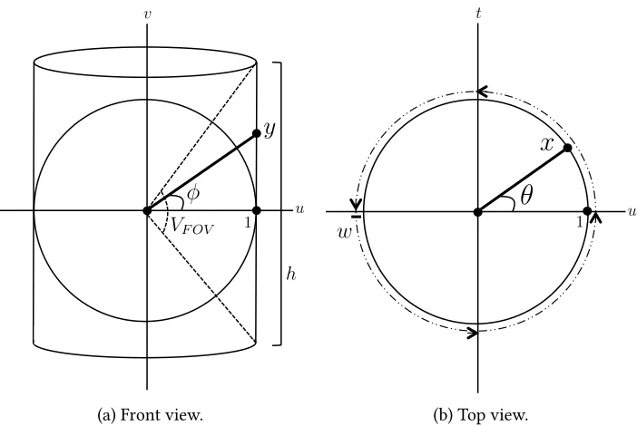
To compute a cylindrical projection, ray trace from the center of projection through a cylinder centered about that point out until an intersection with one or more images. en, color that

particular pixel on the cylinder with the color determined by the rendering algorithm for the

pixels from original images that lie along this ray (Figure.). For a cylindrical projection with

(38)

[image:38.612.90.522.73.291.2]

Figure .: Equirectangular (spherical) rendering of the panorama taken at the Ubehebe Crater in California. e black areas represent portions of the sphere where image data was not captured.

latitude,𝜙, by,

𝑥 = 𝑤

2 1 + 𝜃 𝜋

𝑦 = ℎ

2 1 − tan 𝜙 tan𝑉𝐹𝑂𝑉

2

(.)

where−𝜋 ≤ 𝜃 ≤ 𝜋 and−𝑉_𝐹𝑂𝑉 ⁄ 2 ≤ 𝜙 ≤ 𝑉_𝐹𝑂𝑉 ⁄ 2.

A similar procedure is used for planar projection, replacing the cylinder with a plane

gener-ating a particular ﬁeld of view placed about the center of projection (Figure .). For a planar

projection with a vertical ﬁeld of view,𝑉_𝐹𝑂𝑉 < 𝜋 and a horizontal ﬁeld of view𝐻_𝐹𝑂𝑉 < 𝜋the𝑥

and𝑦coordinates are related to the longitude,𝜃, and the latitude,𝜙, by,

𝑥 = 𝑤

2 1 + tan 𝜃_tan𝐻𝐹𝑂𝑉 2

𝑦 = ℎ

2 1 − tan 𝜙 tan𝑉𝐹𝑂𝑉

2

(.)

(39)

VF OV

y

u

h

1

(a) Front view.

1 u

x

✓

w [image:39.612.132.483.81.316.2]

(b) Top view.

Figure .: Spherical to Cylindrical Panorama Projection Diagram

Any of these methods naturally introduces some amount of geometric distortion. e trade oﬀ is between generating a physically accurate representation of the scene according to the human

visual system and creating a ﬁeld of view large enough to be representative of the geology in the scene.

4.1.2 Rendering Methods

Aer choosing the desired projection method, the panorama can be rendered to an image ﬁle. Autopano Giga has a smart blending algorithm built in that automatically blends overlapping

photos from the panorama. e algorithm detects and removes ghosting and motion artifacts and guarantees a smooth transition between any exposure or color change between images. e

algorithm is multi-threaded and GPU accelerated which speeds up the process signiﬁcantly. If ex-ported at full resolution, it is possible to create panoramas with resolutions of several gigapixels.

(40)

VF OV

y

u

h

1

(a) Front view.

u

1

x

✓

w

HF OV

[image:40.612.131.481.79.315.2]

(b) Top view.

Figure .: Spherical to Planar Panorama Projection Diagram

4.2 Video to Panorama Registration

e purpose of registering the scene video to the high resolution panorama is to be able to have a common reference frame for analysis of the eye-tracking data. What this means is that instead

of analyzing gaze data on an individual basis, the gaze data from a group of observers can be seen and analyzed simultaneously on a single reference image. e diﬃculty in doing this is in part

because every scene video and the panorama itself are captured from a diﬀerent point of view relative to the scene and each other, and in part because the image quality of the scene videos is

vastly inferior to the image quality of the panorama.

A baseline method for accomplishing this task relies on the mathematical matrix

transforma-tion known as a homography. It is a linear projective mapping that takes points from one plane and maps them to another. When applied to images and video taken of a scene, it can transfer

points from one image to another via an intermediate scene plane. us, each video frame should have a homography mapping it to the panorama. It works under the assumption that the images

(41)

us-ing a spherical projection, and there usually isn’t a sus-ingle common scene plane present to identify

feature points with. Additionally, the diﬀerent viewpoints create problems with occluded scene information. However, in many outdoor scenes the features of importance are far away and the

parallax between a given scene video and the panorama is negligible in that region. In this case it is the plane at “inﬁnity” that acts as the intermediate scene plane. ough even if this isn’t the

case, the matching process can still be aempted.

4.2.1 SIFT Feature Tracking

Before matching video frames to the panorama, a scene video is analyzed to determine the frame

to frame image transformations. is allows for the calculation of temporally consistent and smooth results when matching individual video frames to the panorama. To do this, SIFT

fea-tures are computed and matched between each frame and its neighbor using the VLFeat toolbox. Generally there are a large number of outliers aer matching and they need to be ﬁltered out

according to a speciﬁc image transformation model. Since the change in baseline frame to frame in a video is small with a negligible amount of parallax, a homography model can be used to

approximate the transformation from one frame to the next. Using functions from Peter Kovesi’s

computer vision and image processing toolbox [], the putative SIFT matches are passed to a

RANSAC procedure that uses this model to determine a set of matches which are inliers to the model. It is these matches that are used to compute the homography. A record is kept of the

inlier matches from frame to frame so that feature tracks can be determined during processing. e videos and initial SIFT data are put through a second-pass version of this method that

uses only the SIFT features that last through a minimum speciﬁed number of frames to recom-pute the frame-to-frame homography transformations. is method promotes the use of robust

SIFT features and ignores those noisy features which disappear quickly. Figure .graphically

demonstrates SIFT tracking performed on a particular video frame. e diﬀerent colors represent

(42)

[image:42.612.162.453.74.269.2]

Figure .: A visualization of SIFT feature tracking on a video frame. e diﬀerent colors repre-sent how many frames the tracks have survived.

4.2.2 Keyframe Selection

Now that the frame-to-frame homographies have been computed for the scene video, video to

panorama registration can be aempted. Each frame of the scene video needs to be related to the panorama by some kind of spatial transformation. As discussed above, a homography model

can be used to accomplish this. One way to do this for the entire video sequence is to select a single keyframe from the video that will act as a homography anchor to the panorama. Let

the keyframe be given by the 𝑘th video frame and let the current video frame be the 𝑗th. To

compute the appropriate homography for every other video frame, compose each frame-to-frame

homography between the given frame and the keyframe followed by applying the homography from the keyframe to the panorama,𝑯_𝑘,𝑝. en (if𝑗 < 𝑘),

𝑯_𝑗,𝑘 = 𝑘−1

𝑙=𝑗 𝑯_𝑙,𝑙+1

𝑯_𝑗,𝑝 = 𝑯_𝑘,𝑝𝑯_𝑗,𝑘. (.)

A similar procedure works for when 𝑗 > 𝑘. e ﬁrst computation will yield a homography

relating the given frame to the keyframe, 𝑯_𝑗,𝑘, and the second computation will upgrade that

(43)

ensures that the smoothness of the frame-to-frame transformations is preserved when mapping

each video frame to the panorama. e drawback, however, is that the further a given frame is from the keyframe that anchors the video to the panorama, the less accurate the transformation

becomes. is phenomenon is called dri (because the solution is driing away from what is desired) and is mainly caused by accumulations of very small errors in the frame-to-frame

ho-mographies summed over a large number of video frames. e errors themselves are due simply to imperfect data and noise when analyzing the video frames during the SIFT feature tracking

procedure.

To counteract dri in the solution, multiple video keyframes can be selected to anchor the

spatial transformation between the scene video and the panorama. is serves to “reset” the dri that has accumulated at each keyframe, yielding more accurate results. To implement this idea,

the keyframes need to be selected in such a way that they are distributed fairly well throughout the entire video sequence. One way to do this is to simply select a keyframe every certain number

of frames so that there is an anchor at equal time interval during the video.

A more sophisticated method is to use the results of the single keyframe method to inform

the algorithm where to place additional keyframes. By looking at the projective components of the homographies relating each video frame to the panorama, it is possible to determine which

frame in a given time interval is closest to an aﬃne transformation and set it as a keyframe. is is done by analyzing the magnitude of the projective components over time and selecting the local

minima as the keyframes. To avoid geing a keyframe too oen, a parameter is used to smooth the data slightly before computing the local minima. is smoothing parameter essentially controls

the desired keyframe density of the result.

Once the set of keyframes has been selected, each of them needs to be matched to the panorama

with a homography transformation. is is done in the same way as computing the frame-to-frame transformations in the video sequence, with just a few changes. First, SIFT features are

computed for the panorama which will be used for every video keyframe analysis. en, for each keyframe, SIFT features are computed and RANSAC with a homography model is run to

(44)

frames and the panorama that this procedure as it stands will typically fail.

What has been found to work more robustly is to do SIFT feature detection going through ever increasing levels per octave of computation. us, the ﬁrst computation compares SIFT

features detected at three levels per octave to see if a valid homography can be determined using RANSAC. If not, the procedure is repeated at four levels per octave all the way up until twelve

levels per octave if necessary. Once a valid homography is found, the process repeats for the next keyframe. In the case that no valid homography is found, the algorithm resorts to asking for a

manual selection of control points that match between the video frame and panorama. At this point the user also has the option of rejecting that particular keyframe entirely and moving onto

the next one.

4.2.3 Final Homography Calculation

Once the keyframe to panorama homographies have been calculated, the frame to panorama

homographies for all other video frames are computed by composing the frame-to-frame

homo-graphies with the neighboring keyframe to panorama homohomo-graphies. us, if𝑘₁ represents the

previous keyframe,𝑘₂represents the next keyframe and the current frame is the𝑗th, there will

be two frame to panorama homographies given by,

𝑯_𝑗,𝑘

1 = 𝑘1+1

𝑙=𝑗 𝑯_{𝑙,𝑙−1}

𝑯_𝑗,𝑝₁ = 𝑯_𝑘₁_,𝑝𝑯_𝑗,𝑘₁ (.)

𝑯_𝑗,𝑘₂ = 𝑘2−1

𝑙=𝑗 𝑯_𝑙,𝑙+1

𝑯_𝑗,𝑝₂ = 𝑯_𝑘₂_,𝑝𝑯_𝑗,𝑘₂. (.)

To ensure a smooth transition between keyframes and to counter any errors due to dri, the

(45)

using its surrounding keyframes, weighted by the distance to each keyframe,

𝑯_𝑗,𝑝 = 𝛼(𝑗)𝑯_𝑗,𝑝₁ + 𝛽(𝑗)𝑯_𝑗,𝑝₂ (.)

𝛼(𝑗) = 𝑘2− 𝑗 𝑘₂− 𝑘₁ 𝛽(𝑗) = 1 − 𝛼(𝑗).

e ﬁnal set of video frame to panorama homographies can then be used to visualize the scene

[image:45.612.90.524.271.381.2]

video and eye-tracking data onto the panorama (Figure.).

Figure .: A visualization of a frame of the scene video mapped onto the panorama via its ho-mography.

4.2.4 Ground Truth Evaluation

To determine how well this algorithm is performing there needs to be a way of comparing its

results against a ground truth measurement. Unfortunately, accurate ground truth data isn’t available so the alternative is to visually create some approximate ground truth data. To do this,

nine control points representative of the important scene content were manually selected in a panorama of Inspiration Point that would be visible throughout a particular  second video

sequence (Figure .). en, points were located manually in the video sequence that matched

the panorama control points (if visible) for every ten frames.

With this new set of data and the previous set of video to panorama homography

transfor-mations, a measurement of error can be computed. is error, 𝐸, is deﬁned geometrically as

the Euclidean distance (in pixels) between the manually selected point in the 𝑗th video frame,

(46)

Point 3 Point 4 Point 5 Point 6 Point 7 Point 8 Point 9

Figure .: e nine control points selected for use in the ground truth evaluation of the scene at Inspiration Point, Yosemite National Park, California.

appropriate control point,𝒑, in the panorama [],

𝒙_𝑗 = 𝑯𝑗,𝑝𝒙𝑗

𝐸 = 𝒑 − 𝒙_𝑗 . (.)

Ideally they will each be the same point and the error value will reduce to zero pixels. In reality,

0 40 80 120 160 200 240 280 320 360 400 440 480 520 560 600 640 680 720 760 800 840 880 920 960 1000 0 5 10 15 20 25 Frame Number Error [pixels]

Geometric Projection Error

[image:46.612.94.521.77.186.2]

Point 1 Point 2 Point 3 Point 4 Point 5 Point 6 Point 7 Point 8 Point 9

Figure .: e geometric projection error in pixels on the panorama, computed from the manual points selected in each video frame corresponding to each of the nine control points.

the results are not perfect and have a variable amount of error, as ploed in Figure.. e error

(47)

[image:47.612.79.538.77.194.2]

Point 3 Point 4 Point 5 Point 6 Point 7 Point 8 Point 9

Figure .: Plot of the mapped video points for each of the nine control points.

Most of the mapped video points lie within a distance of about  pixels to their respective

control point on the panorama. It turns out the points that have errors that go high oﬀ the chart are due to user mistakes when ﬁnding the control points in the video sequence. Looking at the

raw data it is easy to see that a control point other than the one that was being worked on was

selected, causing those enormous errors. Figure .shows the mapped video points ploed on

the panorama for each of the control points and Figure. shows a close-up view of the area

around each control point. Notice how some of the control points have mapped points whose

colors do not match; this is due to the user error in selecting the correct control point. e rest of the data (ignoring mistakes) lie between a distance of about  and  pixels to their respective

control point. us, a majority of the mapped points are matched well to their control point, however around each there is a scaered amount of poorly matched points (within the  pixel

range). Figure.shows box plots of the statistical distribution of geometric projection errors

corresponding to each of the nine control points. On each box, the center line represents the

median, the edges of the box are the th and th percentiles, the whiskers extend to the most extreme data points not considered outliers, and supposed outliers are ploed individually.

It should be possible to improve these results further by ﬁrst removing the lens distortion present in the scene videos and by using a portion of the panorama that can be rendered

(48)

(a) Control Point 

(b) Control Point 

(c) Control Point 

(d) Control Point 

(e) Control Point 

() Control Point 

(g) Control Point 

(h) Co