Online Tensor Robust Principal Component Analysis

Online Tensor Robust Principal

Component Analysis

Michael Wijnen

A thesis submitted in partial fulfillment for the

degree of Honours in Statistics

at the

Research School of Finance, Actuarial Studies & Statistics

The Australian National University

Supervisor

Dr. Dale Roberts

Declaration

Acknowledgements

Abstract

Contents

1 Introduction 1

1.1 Literature Review . . . 2

1.2 Aims . . . 5

2 Tensors 6 2.1 Basics . . . 7

2.2 Diagonalisation . . . 13

2.3 Factorisation . . . 14

2.4 Norms . . . 17

2.5 Optimisation . . . 22

2.6 Some Useful Derivatives . . . 23

2.7 SVD vs t-SVD Dimensionality Reduction . . . 26

3 Tensor Robust Principal Component Analysis 29 3.1 Projections . . . 32

3.2 Proof that TRPCA Works . . . 40

3.2.1 Construction and Verification of the Dual Certificate . . . 45

3.2.2 WL _{Part 1 . . . . 47}

3.2.3 WL _{Part 2 . . . . 54}

3.2.4 WL _{Part 3 . . . . 56}

3.2.5 WS _{Part 1 . . . . 57}

3.2.6 WS _{Part 2 . . . . 61}

3.3 Discussion and Numerical Experiments . . . 64

4 An Online Algorithm 68 4.1 Reframing the Nuclear Norm . . . 69

4.2 Algorithm . . . 76

4.3 Analysis of Convergence . . . 81

4.4 Discussion of Result . . . 95

4.5 Implementation . . . 98

List of Figures

1.1 Simple Decomposition Problem . . . 2

2.1 Satellite Image of Denman Prospect, Wright, and Coombs (Canberra). . 26

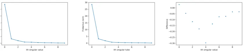
2.2 Singular Values and Singular Tubes . . . 27

2.3 Projected Data . . . 28

3.1 Simple Demonstration of TRPCA . . . 64

3.2 Effect of Varying Rank, Size and ρ on Recovery Error for Normal Noise. . 65

3.3 Effect of Varying Rank, Size and ρ on Recovery Error for Folded Normal Noise . . . 66

3.4 Effect of Permuting Dimensions . . . 67

4.1 TakingT =n2 Large . . . 97

4.2 Cloud Removal . . . 98

Chapter 1

Introduction

In many fields of modern data analysis, the observed data are not necessarily the prime objects of interest. The computer steering a driverless car should pay more attention to objects moving across the foreground (for example, a kangaroo about to jump onto the road) rather than less relevant aspects of the background (for example, a tree far from the road). In the opposite scenario, we might be interested primarily in the background: when we view satellite images, we are often much more interested in the land that lies beneath clouds than we are in the clouds themselves. In addition to this, sensor failures or malicious tampering may also lead us to doubt the quality of observed data. One way of framing this problem is that if the object of our interest, L0, becomes corrupted by

some type of noise, C0, what we observe is then M0 = L0 +C0. A surprising result is

that it is possible to recoverL0 and C0, provided that L0 is of low rank andC0 is sparse.

To do this, we solve the optimisation problem

min

L, CkLk∗+λkCk1, s.t. M0 =L+C.

value decomposition (SVD) or nuclear norm.

1.1

Literature Review

There is a rich body of literature from robust statistics concerning the problem of a lack of faith in the model that is assumed to have generated the observed data (Huber & Ronchetti, 2009; Maronna, Martin, & Yohai, 2006). However, the approach from this lit-erature is not always optimal for two reasons. First, these approaches do not return the best answer. Typically under the regime described above, the goal is to derive estimators to make inferences about the object of interest (L0 in our above formulation), based on

observed data (M0) that are robust to perturbations from noise (C0). In most cases, while

these estimators preserve some desirable properties in the presence of perturbations, they rarely return the ‘correct’ answer that would be returned if there were no perturbations (T. Zhang & Lerman, 2014). Nor should they: based on the assumptions behind these estimators (which typically do not include our assumption that the object of interest is low-rank and the noise is sparse), expecting a ‘correct’ answer would be unreasonable. Second, there are many cases where the object of interest is the perturbation, so in this case, most traditional approaches from robust statistics are not helpful.

As alluded to above, the goal we have in mind is exact recovery of the low rank matrixL0,

which in turn implies exact recovery of the sparse matrix C0. How might one go about

doing this? In the case shown in Figure 1.1, performing this decomposition appears very straight forward.

Figure 1.1: Decomposition into low rank and sparse parts from A. C. Sobral (2017).

way to formalise the perhaps subconscious process of splitting these components is the following optimisation problem

Minimise : rank(L) +λkCk0

Subject to : M =L+C

where k · k0 is the l0 ‘norm’ (this function returns the number of non-zero entries in its

argument, but despite its notation it is actually not a norm). This approach seems intu-itive: we put as much ofM as possible into L while keeping the rank ofL low. However, this optimisation is non-convex, and determining the smallest number of entries that need to be changed to reduce a matrix’s rank (known as a its rigidity) is in general an NP-hard problem (Codenotti, 2000).

We can relax this intractable problem to a tractable convex optimisation by replacing the rank with the nuclear norm (given by the sum of the matrix’s singular values) and by replacing thel0 norm with thel1 norm (given by the sum of the absolute values of the elements of a matrix). One definition of the rank of a matrix is the number of its non-zero singular values, so the rank of a matrix is, in a sense, a version of the nuclear norm that ignores the magnitudes of the singular values. We can be more explicit about the relation between the rank and the nuclear norm: the nuclear norm is the lower convex envelope of the rank (Fazel, 2002). Similarly, the difference between the l0 norm and

the l1 norm is that the l1 norm includes the magnitudes of the elements. For many

Sanghavi, Parrilo, & Willsky, 2011)

Minimise : kLk∗+λkCk1

Subject to : M =L+C

wherek · k∗ is the nuclear norm andk · k1 is thel1 norm. This method has become known

in the literature as Robust Principal Component Analysis, though its only relation to Robust Statistics is in the problem’s set-up and its only relation to Principal Component Analysis is its exploitation of low-dimensional representations.

Under this convex relaxation, many results (Wright et al., 2009; Cand`es et al., 2011; Chandrasekaran et al., 2011; Xu, Caramanis, & Sanghavi, 2012) have been derived that, under certain assumptions on the structure of the data, the matrix L can be exactly recovered with a high probability so long as its rank is sufficiently small. Another useful contribution to this theory was an online stochastic optimisation algorithm developed by Feng et al. (2013) that removes the requirement to load the entire dataset into memory at once, which is particularly useful for large or high-dimensional datasets.

Since these 2-dimensional methods were developed, our understanding of tensors and multidimensional data has grown. In particular, the development of a tensor multipli-cation known as the ‘t-product’ that generalises matrix multiplimultipli-cation has spurred the development the ‘t-SVD’, which generalises the Singular Value Decomposition to the tensor case (Kilmer & Martin, 2011; Martin et al., 2013). These new methods have fa-cilitated the derivation of a new tensor nuclear norm (Lu et al., 2018) that can then be used to extend the previously derived Robust Principal Component Analysis methods to the tensor case. Inspired by Feng et al. (2013), Z. Zhang et al. (2016) also extended the online optimisation algorithm from the 2-dimensional case to the 3-dimensional case, but no proof of convergence was given.

There have also been other approaches employed to apply the Robust Principal Compo-nent Analysis technique to multidimensional data without using the t-product. These are primarily based on the higher-order singular value decomposition (Tucker, 1966), in-cluding online approaches (A. Sobral, Javed, Jung, Bouwmans, & Zahzah, 2015; Li et al., 2018). Though relevant, these techniques are unfortunately beyond the scope of this thesis.

1.2

Aims

Chapter 2

Tensors

A real vector lives in_Rn1 _{and a real matrix in}

Rn1×n2_{. We can generalise this further:}

Definition 2.1. Ap-dimensional real tensor is an element of the vector space _Rn1×...×np_.

In the same way that matrices are much more than just elements of a vector space (for one, they are also linear functions), tensors are also more than just data structures. Our aim in this chapter is to extend to tensors many of the properties that matrices can have, such as invertibility, orthogonality and various factorisations, as well as to derive some basic results for use throughout the later chapters. Much of this work is based on the work of Martin et al. (2013).

First, some notation. In the matrix case, if we have a matrixAinn1×n2, we identify an

element ofA by writing A(i, j) for the element in the ith row andjth column. Similarly we can select the ith row vector of A by writing A(i,:). We extend this idea to tensors in the same way. If A is a tensor in n1×...×np, and J = j1, ..., jp we can select the element in the Jth position AJ = A(j1, ..., jp). We can also select a lower-dimensional data structure by fixing some indices and varying over the others. If we only fix the qth index toiwe will denote thep−1 dimensional data structure asAq_i. Often we will fix only the last dimension, so for simplicity we will write Anp

be taken modulo the size of that dimension. Finally, it will often be convenient to use the following notation: Πp_i=kni ≡n˜k.

2.1

Basics

To talk about things like invertibility, orthogonality and factorisations in a tensor context, we will need a way of multiplying tensors. The following definitions establish the basics needed to do this.

Definition 2.2. The function unfold :n1×...×np →n1np ×n2×...×np−1 is defined

by

unfold(A) =



       

A₁ A₂ .. . A_n

p



       

and has inverse fold:n1np ×n2×...×np−1×N→n1×...×np defined by

fold(unfold(A), np) =A.

In most cases, the second argument of fold will be implied to be np by the fact that it is folding upunfold’s output. Unless it is ambiguous, this argument will not be included.

Next, we have the circulant operator.

Definition 2.3. The functionbcirc:n1np×n2×n3×...×np−1 →n1np×n2np×n3×...×np−1

is defined for a block vector of tensors (or just a normal vector)

A=



       

A1

A2

.. . Anp



where each Ai is in n1×...×np−1 (and in all cases we will be considering, A will be the

output of unfold) as

bcirc(A) =



       

A1 Anp Anp−1 . . . A2 A2 A1 Anp . . . A3

..

. . .. . .. . .. ... Anp Anp−1 . . . A2 A1



       

.

We also note that we can define an inverse on the range ofbcircbybcirc−1(bcirc(A)) = A, which is well defined because bcirc(A) = bcirc(B) if and only if A = B. Now we can define the t-product.

Definition 2.4. The operation ∗ takes a tensor in n1×n2×...×np and another in

n2 ×l×n3×...×np and then returns a tensor in n1×l×n3×...×np. It is defined for tensors of dimension-3 as

A ∗ B =fold

bcirc unfold(A)

·unfold(B)

where · is normal matrix multiplication. For tensors in dimension greater than 3, the t-product requires the ∗ operation and is defined as

A ∗ B =fold

bcirc unfold(A)

∗unfold(B).

Here, it worth noting which tensors we can multiply with the t-product. They must both be of the same dimension (just like matrices, which are always dimension-2). The size of the second dimension of the first tensor must be same size as the first dimension of the second tensor (just like matrices). The second dimension of the second tensor can be anything it wants (just like matrices). The remaining dimensions must all be the same, which is vacuously true of matrices since the additional dimensions do not exist.

all cases to which we apply the∗operator in the following analysis, we will apply unfold

andbcircmany times to get to the base case. So unless stated otherwise, forAinn1×...× np, we will writebcirc(A) = (bcirc◦unfold)p−2(A) andunfold(A) =unfoldp−2(A).

Lemma 2.5. For Ainn1×n2×...×np, when consideringbcirc(A)as ann˜3×n˜3 block

matrix with blocks of size n1×n2, the ijth block of bcirc(A) is given by

bcirc(A)ij =A(:,:, J)

where the kth dimension of J is given by

i mod˜nk

˜

nk+1

−

j mod˜nk

˜

nk+1

modnk

and n˜p+1 = 1.

Proof. We proceed by induction. For the 3-dimensional case this is saying that

bcirc(A)ij =A

:,:,

i

˜

nk+1

−

j

˜

nk+1

modnk

which follows directly from the definition of the circulant. Now we assume this is true for any p−1 dimensional tensor. Considering blocks of size n1n˜4×n2n˜4, we have that

bcirc(A)ij belongs to the block in row

j

i

˜

n4

k

and column j_n˜j 4

k

, which by the circulant structure is given by the j_˜ni

4

k

−j_n˜j 4

k

modn3th frontal slice of bcirc

p−3_{(A). We then}

need the element in row i modn˜4 and column j modn˜4 of this matrix. But this is the block circulant of the p−1 dimensional tensor

A

:,:,

i

˜

n4

−

j

˜

n4

modn3,:, . . . ,:

so we can apply the inductive hypothesis and we are done.

Lemma 2.6. The Jth frontal face of C =A ∗ B is given by

C(:,:, J) = X I

A(:,:, I)B(:,:, J−I).

Proof. This follows because the indices of the Mth row of bcirc(A) are given by

M modn˜k

˜

nk+1

−

j modn˜k

˜

nk+1

modnk

and the indices for the column of unfold(B) are given by

i mod˜nk

˜

nk+1

−

0 mod˜nk

˜

nk+1

modnk =

i mod˜nk

˜

nk+1

modnk.

So adding these indices together wheni=j (as would be the case in this multiplication) we get the sum of the indices of the frontal slices that are multiplied is constant.

Proposition 2.7. The t-product is associative: A ∗(B ∗ C) = (A ∗ B)∗ C.

Proof. Matrix multiplication, which is the base case of the recursion of the t-product, is associative.

We can now start talking about tensor extensions of familiar matrix properties. First, we define the equivalent of an identity matrix.

Definition 2.8. The order-pidentity tensor inn1×n1×n3×...×np is the tensor I such that I(:,:,0) is then1×n1 identity and any other frontal slice I(:,:, J) is 0.

To see that this does indeed behave like an identity, we note that bcirc(I) = I.

Second, we define the tensor equivalent of a matrix inverse. Like matrices, tensors must be square in the first two dimensions to be invertible.

Definition 2.9. If I,A and B are in n1×n1×n3×...×np and

then B is the inverse of A (and vice versa).

Lemma 2.10. Just like matrices, (A ∗ B)−1 _=B−1_{∗ A}−1_.

Proof. I =A ∗ B ∗ B−1_{∗ A}−1 _=B−1_{∗ A}−1_{∗ A ∗ B.}

Third, we define the equivalent of a matrix transpose. At first glance, this appears to be a weird definition. We introduce it in line with Martin et al. (2013), and then show it is equivalent to another (perhaps nicer) definition.

Definition 2.11. If A is an order-3 tensor inn1×n2×n3 then AT is the order-3 tensor

inn2×n1×n3 found by taking the transpose of each frontal slice and then reversing the ordering of all but the first frontal slice (see diagram below).

If A is an order-p tensor with p > 3 in n1 ×...×np then AT is the tensor in n2 ×n1× n3×...×np found by reversing the ordering of all but the first frontal block and then by taking the transpose of each frontal block, which gives

AT =fold 

           

          

(A₀)T (A_np−1)T

(A_n

p−2)

T

.. . (A₁)T



          



          

. (2.1.1)

Another characterisation is as follows.

Proposition 2.12. If A is an order-p tensor with in n1×...×np then AT is the tensor

in n2×n1 ×n3×...×np given by

AT_{(:,:, J) = A(:,:,−J)}T_{. (2.1.2)}

Proof. We denote the transpose given by (2.1.2) as (·)T0

tensors and let A be a p-dimensional tensor. By the applying the first definition, the inductive hypothesis and recalling that we take all indices modulo that dimension (so in the ith dimension, −j =ni−j), we have that

AT _=fold

                       

(A₀)T (A_np−1)T (A_np−2)T

.. . (Anp

1 )T

                        =fold                        

(A_np−0)T (A_np−1)T (A_np−2)T

.. . (A_n

p−(np−1))

T                         =fold                        

(A₀)T0 (A₋₁)T0 (A₋₂)T0

.. . (A_−(n

p−1))

T0                        

=AT0_.

Remark 2.13. Note that bcirc(AT) = bcirc(A)T, since

bcirc(AT₎

i,j =AT (:,:, J) =A(:,:,n−J) T

=bcirc(A)T j,i

where the index switch follows because, from Lemma 2.5, the kth dimension of J is given by

i modn˜k

˜

nk+1

−

j modn˜k

˜

nk+1

modnk

so

nk−

imodn˜k

˜

nk+1

−

j mod˜nk

˜

nk+1

modn_k =

j modn˜k

˜

nk+1

−

i modn˜k

˜

nk+1

modn_k.

Now we have all the machinery we need to define orthogonality, which is now simple.

Definition 2.14. A tensorQinn1×n1×n3×...×np is orthogonal ifQT∗Q=Q∗QT =I.

Proposition 2.15. A tensor A is invertible (orthogonal) if and only if bcirc(A) is invertible (orthogonal). Also, bcirc(A−1) = bcirc(A)−1.

Proof. From Corollary 2.22 (proved below), we have thatbcirc(A∗B) =bcirc(A)bcirc(B). Then the following calculation demonstrates the point of invertible tensors

The same calculation yields the desired result for orthogonal tensors.

2.2

Diagonalisation

Now we define an important matrix operation that will be used to diagonalise circulant matrices. This will save is large amounts of computation time and will also help to derive an SVD for tensors. First, we need the following definitions.

Definition 2.16. The Kronecker product ⊗ : (n1×n2)×(n3×n4) → n1n3×n2n4 is

given by

A⊗B =



    

A00B . . . A0(n2−1)B ..

. . .. ...

A(n1−1)0B . . . A(n1−1)(n2−1)B



    

Definition 2.17. The discrete Fourier transform of dimension n, Fn is the matrix with elements (Fn)jk =ωnjk for j, k in 0,1, ...n−1 whereωn=e

i2π n , so

Fn =



       

1 1 1 . . . 1

1 ω ω2 . . . ωn−1

..

. ... ... . .. ... 1 ωn−1 _ω2(n−1) _{. . . ω}(n−1)(n−1)



       

.

We will slightly abuse notation and write

˜

F = √1 ˜

n3

Fnp⊗...⊗Fn3 ⊗In1

, F˜ = √1

˜

n3

Fnp⊗...⊗Fn3 ⊗In2

,

where the dimension of the matrix on the end will be implied by what it is taking the product with. These matrices are orthogonal (Martin et al., 2013). We now have the following important theorem.

Theorem 2.18. [Martin et al. (2013)] If A in n1×...×np then

is a block diagonal matrix with n˜3 blocks, each of size n1 ×n2.

Corollary 2.19. The ith block (for i in 0...˜n3) on the diagonal of tdiag(A) is given by Di = ˜Fiunfold(A) where F˜i is the ith row of F˜.

Proof. First we note that from Theorem 2.18 we can write

tdiag(A) = ˜F bcirc(A) ˜F∗ =bdiag({Di}ni˜=03 )

so, as ˜F∗F˜ =I, we have

˜

F bcirc(A) = bdiag({Di}ni˜=03 ) ˜F

The 0th block column of ˜F is a column of identities, so the 0th block column ofbdiag({Di}˜n3 i=0) ˜F

is{Di}˜ni=03 arranged as a block column. And theith entry of the 0th column of ˜F bcirc(A)

is the ith row of ˜F times the 0th column of bcirc(A) which is given by unfold(A)

(Lemma 2.5).

Lemma 2.20. [Martin et al. (2013)]If D=bdiag({Di}in˜=03 )thenF D˜ F˜

∗ _{has the required}

block circulant structure so that bcirc−1F D˜ F˜∗ =D0 _{for some tensor D}0_.

Lemma 2.21. [Martin et al. (2013)] If C =A ∗ B thentdiag(C) =tdiag(A)tdiag(B).

Corollary 2.22. The bcirc operation has the following property: bcirc(A ∗ B) = bcirc(A)bcirc(B).

Proof. We have that tdiag(C) = tdiag(A)tdiag(B), so cancelling the Fourier trans-forms givesbcirc(A)bcirc(B) =bcirc(C) =bcirc(A ∗ B).

2.3

Factorisation

Theorem 2.23. A p-dimensional tensor A in n1×n2×...×np can be factored as

A=U ∗ S ∗ VT

where U is in n1×n1×n3×...×np and V is in n2×n2×n3×...×np are orthogonal

and S is in n1×n2×...×np with the properties that S(i, j, .., k) = 0 unless i=j and if S(a, a,:, ...,:) = 0, then S(b, b,:...,:) =0 for all b ≥a.

Proof. To see this we use Theorem 2.18 to block-diagonalise and then take the SVD of each block on the diagonal:

˜

F bcirc(A) ˜F∗ =bdiag({Di}ni˜=13 )

=bdiag({Ui}ni˜=13 )bdiag({Si}ni˜=13 )bdiag({V

T i }

˜

n3 i=1)

=bdiag({Ui}ni˜=13 ) ˜FF˜

∗

bdiag({Si}ni˜=13 ) ˜FF˜

∗

bdiag({V_iT}˜n3 i=1)

where Di =UiSiViT. Then we define U =bcirc −1_{( ˜F}∗

bdiag({Ui}ni˜=13 ) ˜F),

S =bcirc−1( ˜F∗bdiag({Si}ni˜=13 ) ˜F), and VT =bcirc

−1_{( ˜F}∗

bdiag({VT i }

˜

n3

i=1) ˜F) (which are

all well defined by Lemma 2.20). Then we have that:

U ∗ S ∗ VT _{=U ∗ S ∗ V}T _{∗ I}

=fold bcirc(U)bcirc(S)bcirc(VT_)unfold(I)

=fold

˜

F∗bdiag({Ui}ni˜=13 ) ˜FF˜

∗

bdiag({Si}ni˜=13 ) ˜FF˜

∗

bdiag({V_i∗}n˜3

i=1) ˜F unfold(I)

=fold

˜

F∗bdiag({Ui}ni˜=13 )bdiag({Si}ni˜=13 )bdiag({V

∗ i }

˜

n3

i=1) ˜F unfold(I)

=fold

˜

F∗bdiag({Ui}ni˜=13 )bdiag({Si}ni˜=13 )bdiag({V

∗ i }

˜

n3

i=1) ˜F unfold(I)

=fold(bcirc(A)unfold(I))

To see that U is orthogonal, we have that

U ∗ UT _{=U ∗ U}T _{∗ I =}

fold(bcirc(U)bcirc(UT)unfold(I))

=fold( ˜F∗bdiag({Ui}ni˜=13 ) ˜FF˜

∗

bdiag({U_iT}n˜3

i=1) ˜Funfold(I)) =I

and a nearly identical calculation shows that V ∗ VT _{=I. The fact that S(i, j, .., k) =0} unless i = j follows because the Fourier transform acts on the blocks of size n1 ×n2,

and so the diagonal structure within the blocks is preserved. The tensor S also has the property that if S(a, a,:, ...,:) = 0, then S(b, b,:...,:) = 0 for all b ≥a. This also follows because the Fourier transform preserves the diagonal structure within the blocks, and these blocks are diagonal matrices from the middle of SVDs (which possess the property that Saa = 0 =⇒ Sbb= 0 for all b≥a).

Remark 2.24. We can define square roots and inverse square roots (when the tensor is invertible) by taking the square roots and inverse square roots of the diagonal matrix with positive values bdiag({Di}n˜3

i=1), and then apply the Fourier transform and inverse

block circulant in the same way that the t-SVD was defined.

Remark 2.25. IfA,Bare in the set {S|S(i, j, .., k) = 0 unlessi=j}thenA ∗ B=B ∗ A.

Proof. Using Lemma 2.6, we can write the t-product as follows, and then use the fact that diagonal matrices commute to get

A ∗ B(:,:, J) =X I

A(:,:, I)B(:,:, J−I) =X I

B(:,:, J−I)A(:,:, I) =B ∗ A(:,:, J)

For this thesis, there are two ways of defining the rank of a tensor that will be useful for us.

Definition 2.26. The tensor average rank ofA=U ∗ S ∗ VT _{in n}

1×...×np is given by

ranka(A) =

1 ˜

n3

rank(bcirc(A)) = 1 ˜

n3

Definition 2.27. The tensor tubal rank of A = U ∗ S ∗ VT _{in n}

1×...×np is given by the number of non-zero tubes of S:

rankt(A) = #{i,S(i, i,:, ...,:)6= 0}= min{rank(Si)}.

The tensor tubal rank will be used a lot more in this thesis, so we will use the word rank to refer to the tensor tubal rank. The two are connected though, with the tensor average rank providing a lower bound for the tensor tubal rank (Lu et al., 2018). So low-rank tensors (referring to low tubal rank), necessarily have low average rank.

Remark 2.28. We can also define a skinny t-SVD. We derive this in the same way as the regular t-SVD except that we use skinny SVDs instead of regular. To ensure that the dimensions line up, we keep rankt(A) singular values and their associated rows and

columns, so these skinny SVDs may be of dimension slightly larger than normal skinny SVDs and may have some zero singular values. In particular, for rankt(A) =r we have

A =U0_{∗ S}0 _{∗ V}0T_{; however, U}0 _{is in n}

1 ×r×n3...×np, V0T is in r×n2×n3...×np and S0 _{is in r×r×n}

3...×np, soU0 andV0 are not orthogonal, thoughU0T∗ U0 =V0T∗ V0 =I is in r×r×n3...×np.

2.4

Norms

Since the tensor optimisation problem at the heart of this thesis involves the minimisation of the sum of two tensor norms, the following definitions and basic results will be used frequently throughout. We start with two simple norms that are very similar to their matrix and vector counterparts.

Definition 2.29. The l1 norm of a tensor A in n1×...×np with indices in J is defined as

kAk1 =

X

J

Definition 2.30. The infinity norm of a tensor A is given by

kAk∞ = max J |AJ|.

Proposition 2.31. hA,Bi=P

JA ∗

JBJ ≤maxJ|BJ|

P

J|AJ|=kBk∞kAk1. Next, we define an inner product for tensors.

Definition 2.32. The inner product of A and B in n1×n2 is given by

hA, Bi=trace(A∗B) = X i,j

A∗_ijBij.

and for A and B in n1 ×...×np it is given by

hA,Bi= np−1

X

i=0

hAnp

i ,B np

i i.

We equivalently can write that

hA,Bi=X J

A∗_JBJ.

To see that these are equivalent, we note first that it is true for the 2-dimensional case by the definition above. Then, proceeding by induction, we assume it is true for thep−1 dimensional case. Then by applying the definition and the inductive hypothesis we get

hA,Bi = np−1

X

i=0

hAnp

i ,B np

i i= np−1

X

i=0

X

J (Anp

i ) ∗ J(B

np

i )J =

X

J

A∗_JBJ.

then noting that

trace(A∗∗ B) = trace(A∗∗ B(:,:,0))

=trace X

J

A∗(:,:, J)B(:,:,0−J)

!

=trace X

J

A(:,:,−J)∗B(:,:,−J)

!

=X

J

trace(A(:,:, J)∗B(:,:, J))

=X

J

A∗_JBJ.

Remark 2.34. The adjoint of tensor multiplication is tensor multiplication by the Her-mitian tensor: hA ∗ B,Ci =hB,A∗∗ Ci. Using the characterisation of the inner product from above, we have thathA ∗ B,Ci=trace(B∗∗ A∗∗ C) = hB,A∗_{∗ Ci.}

Remark 2.35. Because the circulant structure repeats the same elements multiple times, we also have that

hbcirc(A),bcirc(B)i=hbcircp−2(A),bcircp−2(B)i

=n3hbcircp−3(A),bcircp−3(B)i= ˜n3hA,Bi.

Definition 2.36. We defineeJ as the tensor with a 1 in itsJth element and 0s elsewhere.

Remark 2.37. [Z. Zhang & Aeron (2017)] If eJ in n1×...×np withJ =j1...jp then for c

ej1 in n1×1×n3×...×np with c

ej1 = 0 everywhere other than a 1 in (j1,0,0, ...,0),

eJ0 in 1×1×n₃×...×n_p with

r

ej1 = 0 everywhere other than a 1 in (0,0, j3, ..., jp), and r

ej2 in 1×n2×n3×...×np with r

ej1 = 0 everywhere other than a 1 in (0, j2,0, ...,0), then

eJ = c

ej1 ∗eJ0 ∗ r

ej2.

Definition 2.39. The Frobenius norm of a tensor A in n1×...×np is given by

kAkF =

p

hA,Ai=

s X

J

|AJ|2.

From this and the inner product above we get the Cauchy–Schwarz inequality

hA,Bi ≤phA,AiphB,Bi=kAkFkBkF. (2.4.1)

Using Remark 2.35 for the second equality, we get

kbcirc(A)kF =

p

hbcirc(A),bcirc(A)i=p˜n3hA,Ai =

p

˜

n3kAkF. (2.4.2)

Using the matrix bound kABkF ≤ kAkFkBkF and the calculation above we get that

kA ∗ BkF =kbcirc(A)unfold(B)kF ≤ kbcirc(A)kFkunfold(B)kF =pn3˜ kAkFkBkF.

(2.4.3)

Using the other characterisation of the dot product from Remark 2.33, we have that multiplication by orthogonal tensors preserves the Frobenius norm

kQ ∗ Ak2

F =trace(A

∗_{∗ Q}∗ _{∗ Q ∗ A) =}

trace(A∗∗ A) =kAk2_F. (2.4.4)

And finally, using some of the above facts also gives

ktdiag(A)k2_F =kF˜bcirc(A) ˜F∗k2

F = ˜n3kAk2F. (2.4.5)

Now we use the Frobenius norm to define the spectral norm of a tensor.

Definition 2.40. The spectral norm of a tensor A inn1×...×np is given by

kAk= sup kBkF=1

kA ∗ BkF,

Note that this is the operator norm of tensor multiplication, measured by the Frobenius norm (which was induced by the inner product). From this we also note that

kAk= sup kBkF=1

kA ∗ BkF = sup kunfold(B)kF=1

kbcirc(A)unfold(B)kF =kbcirc(A)k. (2.4.6)

And since the spectral norm is induced the by Frobenius norm, which is invariant under multiplication by orthogonal tensors, the spectral norm is invariant under multiplication by orthogonal tensors. In particular,

kAk=kbcirc(A)k=kF˜bcirc(A) ˜F∗k=ktdiag(A)k. (2.4.7)

Also, we use the fact that kA ∗ BkF ≤ √

˜

n3kAkFkBkF (Eq. (2.4.3)) to get

kAk= sup kBkF=1

kA ∗ BkF ≤ sup kBkF=1

p

˜

n3kAkFkBkF =

p

˜

n3kAkF. (2.4.8)

Finally, we are ready to introduce the tensor nuclear norm, which we define as the dual norm of the spectral norm.

Definition 2.41. The tensor nuclear norm of a tensor A in n1×...×np is given by

kAk∗ = sup kBk≤1

hA,Bi.

Remark 2.42. We briefly note a few different ways of writing the tensor nuclear norm

kAk∗ = sup kBk≤1

hA,Bi= 1 ˜

n3

sup kbcirc(B)k≤1

hbcirc(A),bcirc(B)i= 1 ˜

n3

kbcirc(A)k∗,

where the third equality holds by the definition of matrix nuclear norm (as the dual of the matrix spectral norm). Writing the t-SVD of A asA =U ∗ S ∗ VT_{, we also have by} using the definition of the matrix nuclear norm as the sum of its singular values that

kAk∗ = 1 ˜

n3

hF˜bcirc(S) ˜F∗, Ii= 1 ˜

n3

hbcirc(S), Ii=hS,Ii=

rankt(A)−1

X

i=0

S(i, i,0),

which interestingly only depends on the values ofS in the first frontal slice. These values, however are related to all the values in S via its derivation using the Fourier transform. Finally, we also have that

kAk∗ = 1 ˜

n3h

˜

F bcirc(S) ˜F∗, Ii= 1 ˜

n3h

˜

Fbcirc(S)12F˜∗,F˜_bcirc(S) 1

2F˜∗i= 1 ˜

n3k

˜

F bcirc(S)12F˜∗k2 F.

Proposition 2.43. hA,Bi ≤ kBkkAk∗

Proof. Note that

hA,Bi

kBk ≤kCk≤sup1

hA,Ci=kAk∗.

Now that we have the tensor norms and a few basic results, we can start talking about how we will perform tensor optimisation.

2.5

Optimisation

For every differentiable convex functionf, it holds that

We can generalise this idea to non-differentiable functions as follows.

Definition 2.44. g is a subgradient off atx if

f(y)≥f(x) +g(x)T(y−x),

in which case we write g ∈∂f.

This definition allows us to use the below optimisation method, which does not require the objective function to be differentiable.

Theorem 2.45. [Boyd & Vandenberghe (2008)] If f is convex then

f(x∗) = inf

x f(x) ⇐⇒ 0∈∂f(x ∗

).

In this thesis, two subgradients will be of particular use.

Lemma 2.46. [Lu et al. (2018)] The subgradient of the tensor nuclear norm of a tensor

A with skinny t-SVD given by A=U ∗ S ∗ V∗ _is

{U ∗ V∗+W | U∗∗ W = 0, W ∗ V = 0,kWk ≤1}.

Lemma 2.47. [Boyd & Vandenberghe (2008)] The subgradient of the l1 norm at A is

given by

∂kAk1 ={G | kGk∞ ≤1,hG,Ai=kAk1}.

2.6

Some Useful Derivatives

The following derivatives will be useful in the later chapters.

Lemma 2.48. d

dB 1

2kA ∗ Bk

2

F =A

Proof. We have

d dB

1

2kA ∗ Bk

2

F =

d dunfold(B)

1

2kfold(bcirc(A)unfold(B))k

2

F

= d

dunfold(B)

1

2kbcirc(A)unfold(B)k

2

F

= d

dunfold(B)

1

2trace((bcirc(A)unfold(B))

T _{bcirc(A)unfold(B))}

= d

dunfold(B) 1

2trace(unfold(B) T

bcirc(A)T bcirc(A)unfold(B)) =bcirc(A)T bcirc(A)unfold(B)

=AT _{∗ A ∗ B,}

where the second-last line follows from the standard matrix identity (e.g. Roweis (1999)).

Lemma 2.49. d

dA 1

2kA ∗ Bk

2

F =A ∗ B ∗ B T_.

Proof. To show that this is true, we show that every frontal slice is the same on each side of the equality. Using the other characterisation of the t-product from Lemma 2.6 and the standard matrix identity (e.g. Roweis (1999)), we get

d dA(:,:K)

1

2kA ∗ Bk

2

F =

d dA(:,:K)

1 2

X

J

kA ∗ B(:,;J)k2_F

= d

dA(:,:K) 1 2 X J kX I

A(:,:, I)B(:,;J −I)k2_F

=X

J

X

I

A(:,:, I)B(:,;J−I)B(:,;J−K)T

=X

J

X

I

A(:,:, I)B(:,;J−I)BT_{(:,;K −J)}

=X

J

(A ∗ B)(:,;J)BT_(:,;K−J)

= (A ∗ B ∗ BT_)(:,:K).

Definition 2.50. The function tvec : n1 ×...×np → ˜n1 ×1 flattens a tensor into a

vector.

Remark 2.51. Supposef :n1×..×np →Ris infinitely differentiable with third deriva-tive equal to 0. Then Taylor’s theorem gives

f(B) =f(A) +tvec(B − A)T(∇Af(A)) +1

2tvec(B − A)

T_{(∇A∇Af(A))tvec(B − A).}

Formally, calculating the above expansion requires explicitly writing out the Hessian matrix and deciding on an ordering onto which unfoldwill map. In nearly every case in this thesis, this will not be necessary. Instead it is sufficient for our purposes to note that

d

dAunfold(A ∗ B) =bcirc(B)⊗In1 since

d

dA(:,:, L)(A ∗ C)(:,:, K) =

d dA(:,:, L)

X

J

A(:,:, J)C(:,:, K −J)

= d

dA(:,:, L)A(:,:, L)C(:,:, K−L)

= d

dA(:,:, L)A(:,:, L)C(:,:, K−L) =C(:,:, K−L)T ⊗In1.

Arranging these appropriately gives _dAd unfold(A∗C) =bcirc(CT_)⊗I

n1. This means that when∇Af(A) =A∗Cfor some tensorC, by using the fact thatkbcirc(A)kF =

√ ˜

n3kAkF (Eq. (2.4.2)), we get

k∇A∇Af(A)kF =kbcirc(CT)⊗In1kF =n1kbcirc(C T_)k

F =n1

p

˜

n3kCkF.

We will need the explicit expression in one instance. Fortunately, it is the simplest case: ∇Af(A) = A ∗ I = A. In this case we have that d

d dA(K)

d

dA(J)f(A) = 1 whenK =J and 0 otherwise, so the Hessian is given by the identity,

which in particular is positive definite.

2.7

SVD vs t-SVD Dimensionality Reduction

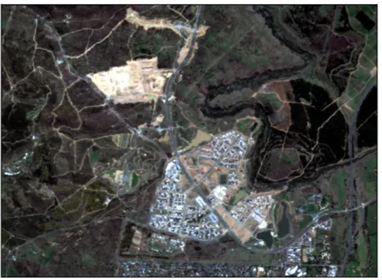
The following example is presented to demonstrate the utility of the t-SVD and its sim-ilarity with the SVD. The pixels of the satellite image in Figure 2.1 are 10-dimensional, but we can only view 3 dimensions at a time. As a result, projecting the 10×565×410 tensor to 3×565×410 in a way that minimises information loss is of great use.

Figure 2.1: The red, green and blue bands of a 10×565×410 Sentinel-2 (recently launched satellite) observation of Denman Prospect, Wright, and Coombs (Canberra) at a single observation date. All of the other satellite images used in this thesis will be of the same area taken by the same satellite.

of A is given by A=U ∗ S ∗ V∗_{, then we can project A to a lower dimension by setting} A0 _=U∗_{(0 : 3,:, . . . ,:)∗ A(see Hao, Kilmer, Braman, & Hoover (2013) for more details).} There are many differences of course. For example, the objects corresponding to singular values in the tensor case are p−1 dimensional. So to measure their size we have to take a norm.

Chapter 3

Tensor Robust Principal Component

Analysis

The goal of this chapter is to prove that the Tensor Robust Principal Component Analysis (TRPCA) procedure does what it says it does: when we observe M0 that is the sum of

a low-rank tensor L0 and a sparse noise tensorC0, the unique minimiser to

min

L,CkLk∗+λkCk1, s.t. M0 =L+C

is (L0,C0). The proof that we give is similar to the proof in Lu et al. (2018), but it

differs in three ways. First, our proof is for tensors of arbitrary dimension rather than 3-dimensional tensors with square frontal faces. Second, our proof is more explicit as it gives specific constants in our bounds rather than leaving them unspecified. Third, our proof takes the probability that an element of the tensor contains noise (ρ) as exogenous (though bounded above by a relatively high bound), rather than relying on it being small to bound some terms. To achieve these results we need to rework many parts of the proofs in Lu et al. (2018). In particular, Lemma D.1 from Lu et al. (2018) was removed from the argument given here and an alternative approach was employed, resulting in a new bound at the end of Section 3.2.5.

the minimisation problem we are addressing. One of the main challenges is that the separation of the low-rank and sparse components of the data becomes intractable if the low-rank part is sparse or if the sparse noise is low rank. To avoid this situation, we assume that the support of the sparse noise is Bernoulli distributed (so then a low-rank sparse noise tensor is highly unlikely). We further assume that the orthogonal tensors in the skinny t-SVD of the low-rank part are not too ‘incoherent’ as measured by µ, which we define as the minimum m for which all of the following conditions (known as tensor incoherence conditions) hold simultaneously:

max j∈0...n1−1

kU∗∗ecjkF ≤

r

mr n1n˜3

, (3.0.1)

max j∈0...n2−1

kV∗∗erjkF ≤

r

mr n2n˜3

, (3.0.2)

kU ∗ V∗k∞≤

r

mr

˜

n1n˜3

. (3.0.3)

The minimum possible value of µ is 1; this would occur when the values of U(i,:, ...:), which are similar to rows of a matrix, are constant at √1

n1˜n3 and the values V(:, i,:, ...,:), which are similar to columns of a matrix, are constant at √1

n2n˜3. The maximum possible value ofµis n(2)n˜3

r ; this would occur when one of the values ofU(i,:, ...:) andV(:, i,:, ...,:) are 1. As µgets smaller, we are seeing the information stored in each ‘row’ or ‘column’ ‘spread out’ across the matrix (and a ‘spread out’ matrix is the opposite of sparse), and so the problem gets easier to solve asµgets smaller (Z. Zhang & Aeron, 2017). The third tensor incoherence condition above is less intuitive than the other two and is regarded by some as restrictive (Chen, 2015); it is, however, necessary for us to be able to solve this problem (Lu et al., 2018).

Theorem 3.1. Suppose that we observe M0 =L0+C0 such that the signs of C0 are ±1

with probability ρ/2 and 0 with probability 1−ρ, the tensor L0 has the skinny t-SVD

U ∗ S ∗ V∗ _andrank

t(L0) =r, the tensor incoherence conditions Eq. (3.0.1) to Eq.(3.0.3)

are satisifed with constant µ, and the following conditions are satisfied (where we write

n(1) = max{n1, n2} and n(2) = min{n1, n2})

ρ < 436−6

√ 836

900 ≈0.2917, (3.0.4)

r≤ρ2 4

54

1

µ

n(2)n˜3

(log(n(1)n˜3))2

, (3.0.5)

then when

λ= _p 1

n(1)n3˜

(3.0.6)

we have that (L0,C0) is the unique minimiser to

min

L,CkLk∗+λkCk1, s.t. M0 =L+C

with ‘high probability’ (which for this thesis will mean greater than 1−O((n(1)n˜3)−1)). Remark 3.2. We will fix ε = µr(log(n(1)n˜3))2

n(2)n˜3

1₄

to yield the following inequalities that will be of use later. First we note that substituting in the bound for µr from Eq. (3.0.5) gives ε <

√

2ρ

5 since

ε=

_µr(log(n

(1)n˜3))2 n(2)n˜3

14 ≤

ρ2 4

54

1₄

=

r

ρ 2

25 < 1

5 <exp(−1) (3.0.7)

where the second-last inequality holds by the fact that we are assuming ρ < 1₂. Rear-ranging the bound for r from Eq. (3.0.5) and substituting in the value we have fixed for

ε gives

C0

−2_µrlog(n (1)n˜3) n(2)n˜3

≤ρ≤1−C0

−2_µr(log(n

(1)n˜3))2 n(2)n˜3

(3.0.8)

right-hand side we have used the fact that ρ < 1−ρ since ρ < 1

2. For this analysis, we

will fix

C0 =

32

3 (3.0.9)

which also loosens these bounds. There are many other choices for the constants that can be made to work. These ones were chosen above to obtain a success probability of 1−O((n(1)n˜3)−1).

Inequalities Eq. (3.0.5) and Eq. (3.0.8) tell us that we need to have a lower bound on the amount of noise for our TRPCA procedure to work, which is counter-intuitive on face value. However, it is logical that for this procedure to succeed we will need a certain amount of noise: if there was no noise, we would observe M0 = L0 +C0 = L0+ 0, and

when we performed the TRPCA procedure min

L,CkLk∗ +λkCk1, s.t. M0 = L+C, we would need its minimum to be at L = M0, C = 0. It seems unlikely that this would

be the case, since some of C0 (corresponding to finer detail/high rank information) will

probably be put into C unless the rank of L0 is very small. We note further that if we

really need a minimum amount of noise, we can just add more noise. The inequality from Eq. (3.0.5) also strangely says that as the amount of noise rises, the required rank can rise. This is very unintuitive, and there appears to be no particular reason for this to be the case. Whether this relationship actually holds will be among the questions explored at the end of this chapter.

3.1

Projections

The proof of Theorem 3.1 relies heavily on two projections, and how they interact. This section introduces these projections and provides some basic results to be used later.

Definition 3.3. We define the projection onto the set of indicesΩ:= support(C0) as

PΩ(A) =

X

J

where δJ = 1 when J ∈Ωand 0 otherwise.

Definition 3.4. We define the spaceT, which is somewhat analogous to the column/row space of the low-dimensional object we are interested in:

T:={U ∗ Y∗+W ∗ V∗| Y∗ ∈_Rr×n2×...×np _{W ∈}

Rn1×r×...×np}.

Definition 3.5. The projection onto T is given explicitly by

PT(A) = U ∗ U∗∗ A+A ∗ V ∗ V∗− U ∗ U∗∗ A ∗ V ∗ V∗,

so that

PT⊥(A) =A −P_T(A)

=A −(U ∗ U∗∗ A+A ∗ V ∗ V∗− U ∗ U∗∗ A ∗ V ∗ V∗) = (I − U ∗ U∗)∗ A ∗(I − V ∗ V∗).

Lemma 3.6. The operators PΩ, PΩ⊥, P_T and P_T⊥ are linear, self-adjoint and have

operator norm less than or equal to 1.

Proof. These projections are all linear because the t-product and inner product are linear. As the sum and composition of self-adjoint operators are self-adjoint, and since PT and

P_T⊥ are defined by the sum of multiple t-products by a Hermitian tensor (which is

self-adjoint), we have thatPT and PT⊥ are self-adjoint. A very simple direct calculation also

shows thatPΩ and PΩ⊥ are self-adjoint. Finally we note that all self-adjoint projections

have norm less than or equal to 1.

Proposition 3.7. kPTeIk2F ≤

µr(n1+n2)

˜

n1 .

Proof. Since PT is self-adjoint (Lemma 3.6) we have that

which then becomes

=hU ∗ U∗∗eI +eI ∗ V ∗ V∗− U ∗ U∗∗eI∗ V ∗ V∗,eIi

=hU ∗ U∗∗eI,eIi+heI∗ V ∗ V∗,eIi − hU ∗ U∗∗eI∗ V ∗ V∗,eIi =hU∗∗eI,U∗ ∗eIi+hV∗∗e∗I,V

∗_∗

e∗_Ii − hU∗∗eI∗ V,U∗∗eI∗ Vi

=kU∗∗eIk2F +kV ∗_∗

e∗_Ik2

F − kU ∗_∗

eI∗ Vk2F

≤ kU∗ ∗eIk2F +kV ∗ _∗

e∗_Ik2

F

=kU∗∗eci1k

2

F +kV ∗_∗ r

ei2k

2

F

where the last equality holds because eJ = c

ej1 ∗eJ0 ∗ r

ej2 (Remark 2.37). Now, since we have max

j∈0...n1−1

kU ∗ecjkF ≤

q _µr

n1˜n3 and _j∈max_0...n 2−1

kV∗ _∗er jkF ≤

q _µr

n2n˜3 (Eq. (3.0.1) and Eq. (3.0.2)) this is less than or equal to

µr n1n˜3

+ µr

n2n˜3

= µr(n1+n2) ˜

n1 .

We will use the following theorem from Tropp (2011) to bound the norm of tensors. It is a generalisation of the classic Bernstein inequality to the non-commutative and random matrix setting.

Theorem 3.8. [Tropp (2011)] Let {Zk}K

k=1 be a sequence of independent n1 ×n2

ran-dom matrices such that _EZk = 0 and kZkk ≤ R almost surely. Then if we let σ2 = maxnkPK

k=1E[Z

∗

kZk]k,kPK_k=1E[ZkZk∗]k

o

we have that for any t≥0,

P K X k=1 Zk ≥t !

≤(n1+n2) exp

− t

2

2σ2₊ 2 3Rt

≤(n1+n2) exp

−3t

2

8σ2

, for t ≤ σ

2

R. Lemma 3.9. If Ω follows a Bernoulli distribution with parameter ρ≥C0−2

µrlog(n(1)n˜3) n(2)˜n3 ,

then

with high probability.

Proof. Our approach will be to bound PT − ρ−1PTPΩPT by writing its norm as the norm of a sum of random matrices and then bounding that expression using the non-commutative Bernstein inequality (Theorem 3.8).

First, by unravelling the definition of PΩ (Remark 2.38) and writing Z as a sum of its elements and basis tensors (Remark 2.38) and then by applying the linearity of PT (Lemma 3.6) and rearranging, we can write

(PT−ρ−1PTPΩPT)Z =PT

X

J

heJZJieJ −ρ−1δJheJ, PTZieJ

!

=X

J

heJZJiPT(eJ)−ρ−1δJheJ, PTZiPTeJ

=X

J

(1−ρ−1δJ)heJ, PTZiPTeJ

≡X J

HJ(Z),

where HJ(Z) = (1−ρ−1δJ)heJ, PTZiPTeJ, which is self-adjoint as

hA,HJ(Z)i=hA,(1−ρ−1δJ)heJ, PTZiPTeJi = (1−ρ−1δJ)heJ, PTZihA, PTeJi =h(1−ρ−1δJ)hPTA,eJiPTeJ,Zi =hHJ(A),Zi.

Now we note that

HJ(Z) =HJunfold(Z)

for somen(2)n˜3×n(2)n˜3 matrix (here, we can usen(2), as transposing preserves the matrix

also have

H_J∗HJunfold(Z) = HJHJ∗unfold(Z) =HJHJunfold(Z)

=HJunfold(HJ(Z))) =HJHJ(Z).

To apply the non-commutative Bernstein inequality (Theorem 3.8) we need to show that

EHJ = 0 and to bound kHJk and kP_JEHJ2k. On the first assumption, we note that

EδJ =ρ soE(1−ρ−1δJ) = 1−1 = 0; hence,EHJ = 0. On the second assumption, since

PT is self-adjoint (Lemma 3.6), we have that

kHJk=kHJk= sup kZkF=1

k(1−ρ−1δJ)heJ, PTZi(PT(eJ))kF

≤ sup kZkF=1

ρ−1|heJ, PTZi| k(PT(eJ))kF

= sup kZkF=1

ρ−1|hPTeJ,Zi| kPT(eJ)kF.

Now we bound this using the Cauchy–Schwarz inequality (Eq. (2.4.1)) and the fact that kPTeJk2F ≤

(n1+n2)µr

˜

n1 (Proposition 3.7) to get

≤ sup kZkF=1

ρ−1kPTeJkFkZkF kPTeJkF

=ρ−1kPTeJk2F ≤ (n1+n2)µr

˜

n1ρ .

Next, we have that

H2

J =HJ(HJ(Z)) =HJ (1−ρ−1δJ)heJ, PTZiPTeJ

= (1−ρ−1δJ)

eJ, PT (1−ρ−1δJ)heJ, PT(Z)iPTeJ

PTeJ

and also that

E(1−ρ−1δJ)2 =E(1−2ρ−1δJ +ρ−2δJ) =ρ−1−1.

So we can combine these to get that

EH2J(Z) = (ρ

−1_−1)he

J, PTZi heJ, PTeJiPTeJ,

and so we can rearrange this using the linearity ofPT (Lemma 3.6) as follows

X J

EHJ2(Z)

F = X J

EH2J(Z)

F = X J

(ρ−1−1)heJ, PTZi heJ, PTeJiPTeJ

F = X J

(ρ−1−1)heJ, PTeJiPT(eJheJ, PT(Z)i)

F ,

and we denote this final expression as (I). Then, to bound (I) we apply the trian-gle inequality. We write maxJ| heJ, PTeJi | = | heM, PTeMi | and recall that PT(Z) =

P

JeJheJ, PT(Z)i (Remark 2.38). From this, we use the fact that PT is a projection to get that

(I)≤(ρ−1−1)| heM, PTeMi |

X J

PT(eJheJ, PTZi)

F

=(ρ−1−1)| heM, PTeMi |

PT X J

eJheJ, PTZi

! F

=(ρ−1−1)| heM, PTPTeMi | kPTPTZkF =(ρ−1−1)| heM, PTPTeMi | kPTZk_F ,

(Eq. (2.4.1)) and the fact that kPTeMk2F ≤

(n1+n2)µr

˜

n1 (Proposition 3.7), we derive

(II)≤(ρ−1−1)| hPTeM, PTeMi | kPTZkF =(ρ−1−1)kPTeMk2FkPTZk_F

≤(ρ−1−1)kPTeMk2FkZkF ≤ρ−1kPTeMk2F kZkF

≤(n1+n2)µr ˜

n1ρ

kZkF

which implies that kP

JEHJ2(Z)k = k

P

JEH2J(Z)k ≤

(n1+n2)µr

˜

n1ρ . Putting the above results together, we get

kPT−ρ−1PTPΩPTk= sup kZkF=1

k(PT−ρ−1PTPΩPT)ZkF

= sup kZkF=1

kX J

HJ(Z)kF

= sup kZkF=1

kX J

HJunfold(Z)kF

=kX J

HJk.

Using the bounds from above with R = (n1+n2)µr n1n2ρ =σ

2 _(so σ2

R = 1> ), we can apply the non-commutative Bernstein inequality (Theorem 3.8) to get

P kPT−ρ−1PTPΩPTk>

=_P kX J

HJk>

!

≤2˜n(2)n˜3exp −

3 8

2 (n1+n2)µr

˜

n1ρ

!

.

We rearrange this final expression and substitute in n1 +n2 ≤ 2n(1) to derive that the

expression is equal to

2n(2)n˜3exp

−3 8

2n˜1ρ

(n1+n2)µr

≤2n(2)n˜3exp

− 3 16

2n˜1ρ n(1)µr

= 2n(2)n˜3exp

− 3 16

2_n (2)n˜3ρ µr

Provided thatρ≥C0−2

µrlog(n(1)˜n3)

n(2)˜n3 , this expression is then

≤2n(2)n˜3exp

−C0

3

16log(n(1)n˜3)

= 2(n(2)˜n3)(n(1)n˜3)−C0

3 16.

Since we choseC0 = 32₃ (Eq. (3.0.9)) we have that this is less than or equal to 2n(2)n−(1)2˜n

−1 3 ,

which is itself less than or equal to O((n(1)n3˜ )−1).

We now prove a proposition that will give us a useful corollary from the lemma above.

Proposition 3.10. kPΩPTk2 =kPTPΩPTk.

Proof. Using the definitions of the relevant norms we get

kPΩPTk2 = sup kAkF=1

kPΩPTAkF

!2

= sup kAkF=1

kPΩPTAk2F = sup kAkF=1

hPΩPTA, PΩPTAi

and then, using the fact that these projections are self-adjoint (Lemma 3.6), we get our desired result:

= sup kAkF=1

hA, PTPΩPΩPTAi= sup kAkF=1

hA, PTPΩPTAi=kPTPΩPTk.

Corollary 3.11. kPΩPTk2 ≤ρ+:=σ < 4₉.

Proof. To see this, we first note that by taking complements in Lemma 3.9, when 1−ρ≥

C0−2

µrlog(n(1)n˜3)

n(2)n˜3 , we get

kPT−(1−ρ)−1PTPΩ⊥PTk ≤.

Next, by rearranging and using the fact that P_Ω⊥ =I −P_Ω we note that

PT−(1−ρ)−1PTPΩ⊥P_T = (1−ρ)−1((1−ρ)P_T−P_TP_Ω⊥PT)

so

PTPΩPT = (1−ρ)(PT−(1−ρ)−1PTPΩ⊥P_T) +ρP_T.

We can then use the triangle inequality and the fact that PT has norm less than or equal to 1 (Lemma 3.6) to get that

kPTPΩPTk ≤(1−ρ)k(PT−(1−ρ)−1PTPΩ⊥P_T)k+ρkP_Tk

≤(1−ρ)+ρ

≤+ρ.

From Proposition 3.10, we have that

kPΩPTk2 =kPTPΩPTk ≤ρ+:=σ.

Then, since from Eq. (3.0.7) we have that ≤ √

2ρ

5 and from Theorem 3.1 ρ <

436−6√836 900 ,

we have that

σ=ρ+≤ρ+ √

2ρ

5 <

436−6√836

900 +

q

2436−6 √

836 900

5 =

4 9.

With these results in hand, we are now ready to begin the main section of this proof.

3.2

Proof that TRPCA Works

To prove that TRPCA works (Theorem 3.1), we will prove the below lemma, which provides a sufficient condition for TRPCA to succeed. Later in this chapter, we will show that this sufficient condition is satisfied when the conditions from Theorem 3.1 are satisfied.

minimi-sation problem with λ= _√ 1

n(1)n˜3

so long as there exists a tensor W satisfying

W ∈T⊥, (3.2.1)

kWk< 1

2, (3.2.2)

kPΩ(U ∗ V∗+W −λsign(C0))kF ≤

λ

4, (3.2.3)

kP_Ω⊥(U ∗ V∗+W)k∞<

λ

2. (3.2.4)

Proof. We will show for any H 6= 0, the objective function that we minimise in TRPCA given by k · k∗ +λk · k1 is larger when evaluated at (L0 +H,C0 − H) than (L0,C0) for

any H. It is sufficient to only consider perturbations of±Has we still have to satisfy the constraint that L+C =M.

First, we fix a W satisfying Eq. (3.2.1) to Eq. (3.2.4). Then we set

E = 1

λU ∗ V

∗ + 1

λW −sign(C0). (3.2.5)

Then we write F =P_Ω⊥E and D=P_ΩE, so by using Eq. (3.2.4), we have that

kF k∞≤ 1

2 (3.2.6)

and by using Eq. (3.2.3), we have that

kDkF ≤ 1

4. (3.2.7)

Substituting this into the above and rearranging, we have

U ∗ V∗+W =λ(sign(C0) +F +D). (3.2.8)

equal to 0 at the minimum.

Now let U ∗ V∗_+W

0 be another subgradient of the tensor nuclear norm atL0 satisfying

hW0,Hi = kPT⊥Hk∗. The existence of such a tensor is guaranteed, as the definition of

the tensor nuclear norm is

kP_T⊥Hk_∗ = sup

kAk=1

hA, P_T⊥Hi.

Since we are taking this supremum over a closed set, there exists a tensor Athat attains the supremum above. Letting W0 = PT⊥A, since P_T⊥ is self-adjoint (Lemma 3.6), we

get

hW0,Hi=hPT⊥A,Hi=hA, P_T⊥Hi=kP_T⊥Hk∗.

We also note that kW0k = kPT⊥Ak ≤ kAk = 1, so U ∗ V∗ +W₀ is an element of the

subgradient of the tensor nuclear norm (Lemma 2.46).

Next, we let sign(C0) +F0 be a subgradient of the the l1 norm atC0 satisfying hF0,Hi=

−kP_Ω⊥Hk₁. The tensor F₀ =−sign(P_Ω⊥H) is an example of such a tensor as

h−sign(PΩ⊥H),Hi =−hsign(P_Ω⊥H), P_Ω⊥Hi =−kP_Ω⊥Hk1.

We also note that the elements of F0 are 0 anywhere sign(C0) is non-zero (as F0 is only

supported onΩ⊥, the complement of the support of sign(C0)); otherwise, the elements of

F0 only equal −1, 0 or 1, so the tensor sign(C0) +F0 is in the subgradient of the l1 norm

atC0 (Lemma 2.47). Then, by applying the definition of subgradients and the equalities

above, we have that

kL0 +Hk∗ +λkC0− Hk1

≥kL0k∗+λkC0k1+hU ∗ V∗+W0,Hi −λhsign(C0) +F0,Hi

So to show that the objective function k · k∗ +λk · k1 is larger when evaluated at (L0+

H,C0− H) than (L0,C0), it is sufficient to show that

hU ∗ V∗−λsign(C0),Hi+kPT⊥Hk∗ +λkP_Ω⊥Hk₁ ≥0.

To do this, we first note that since all the projections in the below expression have norm less than or equal to 1 (Lemma 3.6), and sincekPΩPTk<

√

σ (< 2₃) (Corollary 3.11), we have that

kPΩHkF =kPΩPTH+PΩPT⊥Hk_F

≤ kPΩPTHkF +kPΩPT⊥Hk_F

≤√σkHkF +kPT⊥Hk_F

≤√σkPΩHkF + √

σkPΩ⊥Hk_F +kP_T⊥Hk_F.

We recall thathA,Ai ≤ kAkkAk∗ (Proposition 2.43) andkAk ≤√n˜3kAkF (Eq. (2.4.8)), which we can combine to get

kAk2_F =hA,Ai ≤ kAkkAk∗ ≤pn˜3kAkFkAk∗,

which gives us kAkF ≤ √

˜

n3kAk∗. Then, using this and the fact that kAkF ≤ kAk1, we

have that

(1−√σ)kPΩHkF ≤√σkPΩ⊥HkF +kP_T⊥HkF

≤√σkP_Ω⊥Hk₁ + 2

p

˜

n3kPT⊥Hk∗.

Rearranging Eq. (3.2.8),U ∗ V∗_{+W =λ(sign(C}

kXkkYk∗ (Proposition 2.43), and hX,Yi ≤ kX k1kYk∞ (Proposition 2.31), we get

|hU ∗ V∗−λsign(C0),Hi|=|hλF+λD − W,Hi|

≤ |hλF,Hi|+|hλD,Hi|+|hW,Hi|

=λ|hPΩ⊥F,Hi|+λ|hP_ΩD,Hi|+|hP_T⊥W,Hi|

≤λkP_Ω⊥Hk₁kF k∞+λkP_ΩHk_FkP_ΩDk_F +kP_T⊥Hk∗kWk,

where the last line follows from self-adjointness of PΩ⊥, P_Ω, and P_T⊥. Now we use

kF k∞ ≤ 1₂ (Eq. (3.2.6)), kPΩDkF ≤ 1₄ (Eq. (3.2.7)), kWk ≤ 1₂ (Eq. (3.2.2)) and the result from above that (1−√σ)kPΩHkF ≤

√

σkP_Ω⊥Hk₁+ 2

√ ˜

n3kPT⊥Hk∗ to get that

λkPΩ⊥Hk₁kF k∞+λkP_ΩHk_FkP_ΩDk_F +kP_T⊥Hk∗kWk

≤λ1

2kPΩ⊥Hk1 +λ 1

4kPΩHkF + 1

2kPT⊥Hk∗ ≤λ1

2kPΩ⊥Hk1 +λ 1 4

√

σkPΩ⊥Hk₁ + 2

√ ˜

n3kPT⊥Hk∗

1−√σ +

1

2kPT⊥Hk∗ =kPΩ⊥Hk1λ

1 2+ 1 4 √ σ

1−√σ

+kPT⊥Hk∗

1 2

1 +λ

√ ˜

n3

1−√σ

.

Now we calculate

hU ∗ V∗−λsign(C0),Hi+kPT⊥Hk∗+λkP_Ω⊥Hk₁

≥ − |hU ∗ V∗−λsign(C0),Hi|+kPT⊥Hk∗+λkP_Ω⊥Hk₁

≥ −

kP_Ω⊥Hk₁λ

1 2+ 1 4 √ σ

1−√σ

+kP_T⊥Hk∗

1 2

1 +λ

√ ˜

n3

1−√σ

+kP_T⊥Hk∗+λkP_Ω⊥Hk₁

=kP_Ω⊥Hk₁λ

1− 1 2 + 1 4 √ σ

1−√σ

+kP_T⊥Hk∗

1− 1 2

1 +λ

√ ˜

n3

1−√σ

.

Forλ = √ 1

n(1)˜n3 and √

σ < 2₃, (Corollary 3.11) this becomes

>kPΩ⊥Hk1λ

1− 1 2 + 1 4 2 3

1− 2 3

+kPT⊥Hk∗ 1−

1 2 1 +

1 √

n(1)

1 (1− 2

3)

!!

(3.2.9)

=kP_Ω⊥Hk₁λ(1−1) +kP_T⊥Hk_∗

which is greater than or equal to 0 for everyH(providedn(1) is greater than 9), delivering

our desired result.

3.2.1

Construction and Verification of the Dual Certificate

We will now construct a W that satisfies Eq. (3.2.1) to Eq. (3.2.4) (in the literature, this is known as a dual certificate). To do this, we first note that because the support of C0

(Ω) is assumed to be Bernoulli-distributed with parameter ρ, the distribution of Ωc _is Bernoulli-distributed with parameter 1−ρ, or equivalently

Ωc= j0

[

i=1

Ωi,

for Ωi Bernoulli-distributed with parameterq such thatρ= (1−q)j0_{. To see this we note}

ρ=_P(J ∈Ω) = _P(J 6∈Ωi∀i) =P(Bin(j0, q) = 0) = (1−q)j0.

Rearranging this gives that q = 1−ρj1_{0 ≥} 1−ρ

j0 . Then we choose j0 = dlog(n(1)n˜3)e so that (from Eq. (3.0.8)) we have ρ≤ 1−C0

−2_µr(log(n (1)n˜3))2

n(2)n˜3 , which once rearranged gives us 1−ρ≥C0

−2_µr(log(n (1)n˜3))2

n(2)n˜3 . Hence,

qlog(n(1)n3˜ )≥1−ρ≥C0

−2µr(log(n(1)n˜3))2 n(2)n˜3

,

and in particular

q≥C0

−2_µr(logn (1)n˜3) n(2)n˜3

. (3.2.11)

The last thing we need to do before we construct W is state the following remark.

Remark 3.13. Since kPTPΩk < 2₃ < 1 (Corollary 3.11), on Ω, PΩ−PΩPTPΩ = I −

PΩPT is invertible and (PΩ−PΩPTPΩ) −1

is given by the convergent Neumann series

P∞

k=0(PΩPTPΩ)

Now, we are ready to construct W. To do this, we let

W =WL_+WS _(3.2.12)

where

WS _=λP

T⊥(P_Ω−P_ΩP_TP_Ω)−1sign(C₀) =λP_T⊥

∞

X

k=0

(PΩPTPΩ)ksign(C0) (3.2.13)

(with its inverse being calculated using Remark 3.13) and

WL_=P T⊥Y_J

0 (3.2.14)

for

Yj =Yj−1+q−1PΩjPT(U ∗ V

∗_{− Yj−}

1) (3.2.15)

with Y0 = 0. Substituting W =WL+WS into the conditions Eq. (3.2.1) to Eq. (3.2.4),

the conditions we need to prove become

WL_+WS _∈T⊥

(3.2.16) kWL_+WS_k< 1

2 (3.2.17)

kPΩ(U ∗ V∗+WL+WS −λsign(C0))kF ≤

λ

4 (3.2.18)

kP_Ω⊥(U ∗ V∗+WL+WS)k∞<

λ

2, (3.2.19)

which are satisfied when we satisfy the following sets of conditions for WL

kWL_k< 1

4 (3.2.20)

kPΩ(U ∗ V∗+WL)kF ≤ λ

4 (3.2.21)

kP_Ω⊥(U ∗ V∗+WL)k∞ <

λ

and for WS

kWS_k< 1

4 (3.2.23)

kP_Ω⊥WSk_∞<

λ

4. (3.2.24)

To see this, WL _{and W}S _{are projected onto T}⊥_{, so the constraint in Eq. (3.2.16) will be} satisfied by these new conditions by construction. By the triangle inequality, Eq. (3.2.20) and Eq. (3.2.23) jointly imply Eq. (3.2.17), just as Eq. (3.2.22) and Eq. (3.2.24) jointly imply Eq. (3.2.19). That Eq. (3.2.21) implies Eq. (3.2.18) is a little more complicated, as it relies on the fact that PΩ(WS) =λsign(C0):

PΩWS =λPΩPT⊥(P_Ω−P_ΩP_TP_Ω)−1sign(C₀)

=λPΩ(I −PT) (PΩ−PΩPTPΩ)

−1_sign(C 0)

=λ(PΩ−PΩPT) (PΩ−PΩPTPΩ) −1

sign(C0)

=λ(PΩ−PΩPT) ∞

X

k=0

(PΩPTPΩ) k

!

sign(C0)

=λ(PΩ−PΩPT) ∞

X

k=0

PΩ(PΩPTPΩ) k

!

sign(C0)

=λ(PΩ−PΩPTPΩ) ∞

X

k=0

(PΩPTPΩ)k

!

sign(C0)

=λ(PΩ−PΩPTPΩ)(PΩ−PΩPTPΩ)−1sign(C0)

=λsign(C0).

We will now show that the constructed WL _{and W}S _{satisfy these required constraints,} completing the proof of Theorem 3.1.

3.2.2

W

_{Part 1}

To do this, first we need to prove the following two long lemmas.

Lemma 3.14. If Z ∈T then kZ −ρ−1_P

Proof. To prove this, we will write the expression we want to bound as a sum of random matrices and then bound that sum using the non-commutative Bernstein inequality (The-orem 3.8). We note that by unravelling the definition ofPΩand applying the linearity of

PT we have that

ρ−1PTPΩ(Z) =ρ−1PT

X

J

δJZJeJ

!

=X

J

ρ−1δJZJPT(eJ).

Z ∈T, so PTZ =Z. Noting this, we unravel the definition ofPΩ (Definition 3.3), write Z as a sum of its elements and basis tensors (Remark 2.38) and then rearrange to get

heK,Z −ρ−1PTPΩZi=

*

eK, PTZ −

X

J

ρ−1δJheJ,ZiPTeJ

+

=

*

eK, PT

X

J

heJ,ZieJ

!

−X J

ρ−1δJheJ,ZiPTeJ

+

=

*

eK,

X

J

heJ,ZiPTeJ −

X

J

ρ−1δJheJ,ZiPTeJ

+

=X

J

eK,heJ,ZiPTeJ −ρ−1δJheJ,ZiPTeJ

=X

J

(1−ρ−1δJ)heJ,Zi heK, PTeJi

≡X J

tJ.

We observe that the tJs are independently distributed as they are only stochastic in

δJ. We want to apply the non-commutative Bernstein inequality (Theorem 3.8) (viewing these tJs as 1×1 dimensional matrices), so we need to show that |tJ| and |

P

JE[t

2

J]| are bounded and that _EtJ = 0. First, we note that EtJ = 0 since E(1−ρ−1δJ) = 0. Second, to show that |tJ| is bounded we use that PT is self-adjoint (Lemma 3.6), the Cauchy–Schwarz inequality (Eq. (2.4.1)) and that kPTeIk2F ≤

µr(n1+n2)

˜