C
2014. The American Astronomical Society. All rights reserved. Printed in the U.S.A.
A TECHNIQUE TO DERIVE IMPROVED PROPER MOTIONS FOR
KEPLER
OBJECTS OF INTEREST
∗G. Fritz Benedict1, Angelle M. Tanner2, Phillip A. Cargile3,4, and David R. Ciardi5
1McDonald Observatory, University of Texas, Austin, TX 78712, USA;[email protected] 2Department of Physics and Astronomy, Mississippi State University, Starkville, MS 39762, USA
3Department of Physics and Astronomy, Vanderbilt University, Nashville, TN 37235, USA 4Harvard-Smithsonian Center for Astrophysics, 60 Garden Street, Cambridge, MA 02138, USA
5NASA Exoplanet Science Institute, Caltech, Pasadena, CA 91125, USA
Received 2014 June 20; accepted 2014 August 15; published 2014 October 30
ABSTRACT
We outline an approach yielding proper motions with higher precision than exists in present catalogs for a sample of stars in the Kepler field. To increase proper-motion precision, we combine first-moment centroids ofKepler pixel data from a single season with existing catalog positions and proper motions. We use this astrometry to produce improved reduced-proper-motion diagrams, analogous to a Hertzsprung–Russell (H-R) diagram, for stars identified asKeplerobjects of interest. The more precise the relative proper motions, the better the discrimination between stellar luminosity classes. Using UCAC4 and PPMXL epoch 2000 positions (and proper motions from those catalogs as quasi-Bayesian priors), astrometry for a single test Channel (21) and Season (0) spanning 2 yr yields proper motions with an average per-coordinate proper-motion error of 1.0 mas yr−1, which is over a factor of three better than existing catalogs. We apply a mapping between a reduced-proper-motion diagram and an H-R diagram, both constructed usingHubble Space Telescopeparallaxes and proper motions, to estimateKeplerobject of interestK-band absolute magnitudes. The techniques discussed apply to any future small-field astrometry as well as to the rest of theKeplerfield.
Key words: astrometry – planetary systems – proper motions – stars: distances Online-only material:color figures
1. INTRODUCTION
Astrometric precision,, in the absence of systematic error, is proportional toN−1/2, whereNis the number of observations (van Altena 2013). Theoretically, averaging the existing vast quantity ofKeplerdata might allow us to approachHubble Space Telescope(HST)/Fine Guidance Sensor astrometric precision, 1 ms of arc per observation. WhileKeplerwas never designed to be an astrometric instrument, and despite significant astrometric systematics and the challenge of fat pixels (3.9757 pixel−1), we can reach a particular goal; higher-precision proper motions for Keplerobjects of interest (KOIs) fromKeplerdata. Additionally, these techniques might be useful to future astrometric users of, for example, the Large Synoptic Survey Telescope (Ivezic et al.2008), when they require the highest-possible astrometric precision for targets of interest contained on a single CCD in the focal plane. Finally, proper-motion measurements from any Keplerextended mission might benefit from the application of these techniques.
In transit work, it is useful to know the luminosity class of a host star when estimating the size of the companion. This requires a distance, ideally provided by a measurement of the parallax. With simple centroiding unaware of point-spread function (PSF) structure, the season-to-season Kepler astrometry required for parallaxes presently yields positions with average errors exceeding 100 milliarcseconds (mas), which is insufficient for parallaxes (Section4.3). However, distance is a desirable piece of information. Reduced-proper-motion (RPM) diagrams may provide an alternative distance estimate. The concept is simple: proper motion becomes a proxy for distance (Stromberg1939; Gould & Morgan2003; Gould2004). Statistically, the closer any star is to us, the more likely it is to have a larger proper motion. The RPM diagram consists of the
∗ Based on observations made with the NASAKeplerTelescope.
proper motion converted to a magnitude-like parameter plotted against the color. The RPM diagram is thus analogous to a Hertzsprung–Russell (H-R) diagram. While some nearby stars might have low proper motions, giant and dwarf stars typically are separable. The more precise the proper motions, the better the discrimination between the stellar luminosity classes.
In the following sections, we describe our approach yielding improved placement within an RPM for anyKepler target of interest. In Section2, we outline the utility of RPM diagrams, including a calibration to absolute magnitude derived fromHST astrometry. In Section 3, we discuss Kepler data acquisition and reduction. We present the results of a number of tests providing insight into the many difficulties associated with Kepler astrometry in Section 4. We describe the modeling and proper-motion results for our selectedKepler test field in Section5. We compare our improved RPM with that previously derived from existing astrometric catalogs (Section 5.8), and discuss the astrophysical ramifications of our estimated absolute magnitudes for the over 60 KOI’s in our test field (Section6). We summarize our findings in Section7.
2. A CALIBRATED RPM DIAGRAM
In pastHSTastrometric investigations (e.g., Benedict et al. 2011; McArthur et al. 2010), the RPM was used to confirm the spectrophotometric stellar spectral types and luminosity classes of reference stars. Their estimated parallaxes are input to the model as observations with associated errors. To minimize absorption effects,HSTastrometric investigations useHK(0)=
Table 1
HST MK(0) andHK(0)
No. ID m−M MK(0) SpT μTa K0 (J−K)0 HK(0) Referencesb
1 HD 213307 7.19 −0.86 B7IV 21.82±0.42 6.32 −0.12 −1.98±0.05 B02
2 υAND 0.66 2.20 F8 IV–V 419.26 0.14 2.86 0.32 0.97 0.03 M10
3 HD 136118 3.59 2.00 F9V 126.31 1.20 5.60 0.34 1.11 0.03 Mr10
4 HD 33636 2.24 3.32 G0V 220.90 0.40 5.56 0.34 2.28 0.03 Ba07
5 HD 38529 3.00 1.22 G4IV 162.31 0.11 4.22 0.68 0.27 0.03 B10
6 vA 472 3.32 3.69 G5 V 104.69 0.21 7.00 0.50 2.10 0.03 M11
7 55 Cnc 0.49 3.49 G8V 539.24 1.18 3.98 0.70 2.64 0.03 SIMBAD
8 δCep 7.19 −4.91 F5Iab: 17.40 0.70 2.28 0.52 −6.51 0.09 B07
9 vA 645 3.79 4.11 K0V 101.81 0.76 7.90 0.77 2.93 0.03 M11
10 HD 128311 1.09 3.99 K1.5V 323.57 0.35 5.08 0.53 2.63 0.03 M13
11 γCep 0.67 0.37 K1IV 189.20 0.50 1.04 0.62 −2.58 0.03 B13
12 vA 627 3.31 3.86 K2 V 110.28 0.05 7.17 0.56 2.38 0.03 M11
13 Eri −2.47 4.24 K2V 976.54 0.10 1.78 0.45 1.72 0.03 B06
14 vA 310 3.43 4.09 K5 V 114.44 0.27 7.52 0.63 2.82 0.03 M11
15 vA 548 3.39 4.13 K5 V 105.74 0.01 7.52 0.71 2.64 0.03 M11
16 vA 622 3.09 5.13 K7V 107.28 0.05 8.22 0.84 3.38 0.03 M11
17 vA 383 3.35 5.01 M1V 102.60 0.32 8.36 0.91 3.42 0.03 M11
18 Feige 24 4.17 6.38 M2V/WD 71.10 0.60 10.55 0.69 4.81 0.03 B00a
19 GJ 791.2 −0.26 7.57 M4.5V 678.80 0.40 7.31 0.92 6.47 0.03 B00b
20 Barnard −3.68 8.21 M4Ve 10370.00 0.30 4.52 0.72 9.60 0.03 B99
21 Proxima −4.43 8.81 M5Ve 3851.70 0.10 4.38 0.97 7.31 0.03 B99
22 TV Col 7.84 4.84 WD 27.72 0.22 12.68 0.49 4.89 0.03 M01
23 DeHt5 7.69 7.84 WD 21.93 0.12 15.53 −0.07 7.24 0.03 B09
24 N7293 6.67 7.87 WD 38.99 0.24 14.54 −0.23 7.49 0.03 B09
25 N6853 8.04 2.54 WD 8.70 0.11 10.58 1.13 0.27 0.04 B09
26 A31 8.97 6.69 WD 10.49 0.13 15.66 0.25 5.77 0.04 B09
27 V603 Aql 7.20 4.12 CNe 15.71 0.19 11.32 0.31 2.30 0.04 H13
28 DQ Her 8.06 5.00 CNe 13.47 0.32 13.06 0.46 3.70 0.06 H13
29 RR Pic 8.71 3.54 CNe 5.21 0.36 12.25 0.18 0.83 0.15 H13
30 HP Lib 6.47 7.35 WD 33.59 1.54 13.82 −0.12 6.45 0.10 R07
31 CR Boo 7.64 8.59 WD 38.80 1.78 16.23 −1.52 9.17 0.10 R07
32 V803 Cen 7.70 6.12 WD 9.94 2.98 13.82 −0.10 3.81 0.65 R07
33 Car 8.56 −7.55 G3Ib 15.20 0.50 0.99 0.55 −8.10 0.08 B07
34 ζGem 7.81 −5.73 G0Ibv 6.20 0.50 2.13 0.23 −8.91 0.18 B07
35 βDor 7.50 −5.62 F6Ia 12.70 0.80 2.06 0.48 −7.42 0.14 B07
36 FF Aql 7.79 −4.39 F6Ib 7.90 0.80 3.45 0.40 −7.06 0.22 B07
37 RT Aur 8.15 −4.25 F8Ibv 15.00 0.40 3.90 0.28 −5.22 0.06 B07
38 κPav 6.29 −3.52 F5Ib-II: 18.10 0.10 2.71 0.62 −6.00 0.03 B11
39 VY Pyx 6.00 −0.26 F4III 31.80 0.20 5.63 0.33 −1.86 0.03 B11
40 P3179 5.65 3.02 G0V: 50.36 0.40 8.67 0.35 2.18 0.03 S05
41 P3063 5.65 4.68 K6V: 45.30 0.50 10.33 0.82 3.61 0.04 S05
42 P3030 5.65 4.97 K9V: 43.20 0.50 10.62 0.83 3.79 0.04 S05
Notes.
aμ
T =(μ2RA+μDEC2 )1/2in mas yr−1.
bB99=Benedict et al. (1999), B00a=Benedict et al. (2000a), B00b=Benedict et al. (2000b), B02=Benedict et al. (2002), B06=Benedict
et al. (2006), B07=Benedict et al. (2007), B09=Benedict et al. (2009), B11=Benedict et al. (2011), Ba07=Bean et al. (2007), H13= Harrison et al. (2013), Mr10=Martioli et al. (2010), M01=McArthur et al. (2001), M11=McArthur et al. (2011), R07=Roelofs et al. (2007), S05=Soderblom et al. (2005).
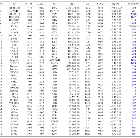
Compared to Hipparcos, HST has produced only a small number of parallaxes and proper motions (Benedict et al. 1999,2000a,2000b,2002,2006,2007,2009,2011; Harrison et al.2013; McArthur et al. 2001,2010,2011,2014; Roelofs et al. 2007), but with higher precision. Parallax and proper-motion results for 42 stars withHSTproper-motion and parallax measures are collected in Table1. Average parallax errors are 0.2 mas. Average proper-motion errors are 0.4 mas yr−1. In Figure1, we compare an H-R diagram and an RPM diagram constructed withHSTparallax and proper-motion results for the targets listed in Table1. Conspicuously absent from the RPM diagram are the RR Lyr results from Benedict et al. (2011) with their large proper motions due to their Halo Pop II identification. Lines plotted on the H-R diagram show predicted loci for
10 Gyr age solar metallicity stars and 3 Gyr age metal-poor stars from Dartmouth Stellar Evolution models (Dotter et al. 2008). These ages and metallicities encompass the majority of what might be expected from a random sampling of stars in our Galaxy.
Even though these targets are scattered all over the sky and range from planetary nebula central stars to Cepheid variables, the similarity between the H-R and RPM dia-grams is striking. In Figure2, we plot the extinction-corrected K-band absolute magnitude derived from HST parallaxes against the magnitude-like parameter HK(0). The resulting
10 5 0 -5
Reduced Proper Motion (H
K(0)
= K
0
+ 5log(
μ
) )
1.2 0.8
0.4 0.0
-0.4
(J-K)0 1
23
4
5
6 7 8
9 10
11
12 13
1415 1617
18
19
20 21 22
23 24
25
26 27
28 29
30 32
33 34
35 36
37
38
39
40
4142
10 5 0 -5
MK
1.2 0.8
0.4 0.0
-0.4
(J-K)0
1
23
4
5
6 7
8
9 10
11
12
13 1415
1617
18
19 20
21 22
23 24
25
26 27
28 29
30 32
33
34 35
36 37
38
39
40
[image:3.612.93.521.56.395.2]41 42
Figure 1.Left: Hertzsprung–Russell (H-R) diagram absolute magnitudeMK(0) vs. (J−K)0, both corrected for interstellar extinction. Plotted lines show predicted loci
for 10 Gyr age solar metallicity stars (- - -) and 3 Gyr age metal-poor ([Fe/H]= −2.5) stars (-··-) from Dartmouth Stellar Evolution models (Dotter et al.2008). Right: RPM diagram, same targets plotted. Horizontal lines separate main sequence and sub-giants, and giants and super-giants. Star numbers are from Table1. The color coding denotes main-sequence stars (red), white dwarfs (blue), and super-giants (black).
(A color version of this figure is available in the online journal.)
Note that while this calibration is produced with proper motions sampling much of the celestial sphere, the H-R diagram and RPM main sequences are defined almost exclusively by stars belonging to the Hyades and Pleiades clusters. This may become an issue when we attempt to apply the calibration to a small piece of the sky in a different location. Both the calibration sources and a randomKeplerfield have systematic proper motions due to galactic rotation (see van Leeuwen2007, Section 6.1.5), which may require some correction.
3.KEPLEROBSERVATIONS AND DATA REDUCTION
The primary mission of the Kepler spacecraft is high-precision photometry which can be used to discover transiting planets.Keplerrotates about the boresight once every 90 days to maximize solar panel illumination. Each such pointing is iden-tified by a season number; 0–3. Each 90 day period is ideniden-tified by a quarter number; 1–17. The CCDs in theKeplerfocal plane are identified by a channel number; 1–84. Our goal is to produce an astrometric reference frame across a givenKepler channel containing KOIs of interest, with the end product being KOI proper motions which can be used to populate an RPM.
3.1. Star Data
TheKeplertelescope trails the Earth in a Sun-centered orbit. Details on the photometric performance and focal plane array
can be found in Borucki et al. (2010) and Caldwell et al. (2010a). The following explorations restrict themselves to the so-called long-cadence data where each subsection containing a star of interest in the array is read out once every 30 minutes. These subsections of theKeplerfield of view (FOV; hereafter, postage stamps) range from 4×5 pixels for fainter stars to larger than 8×8 pixels for brighter stars. Kepler pixels are a little less than 4on a side. Targets observed with long cadence generate approximately 4700 postage stamps per star per quarter.
We obtained our Kepler data from the Space Telescope Science Institute Multimission Archive (MAST). These data include both pipelined positions (the *_llc.fits files, where “*” is a global replacement marker) and postage stamp image data (the *_lpd-targ.fits files). TheKeplerArchive Manual (Fraquelli & Thompson2012) greatly assisted us with any access issues.
3.2. Positions from Kepler Image Data
Positions used in this paper are generated from theKepler postage stamp image data using a simple first-moment centering algorithm. We calculate
MOM CENTRX=i∗z/i, (1)
10 5 0 -5
MK
(0)
10 5 0 -5 -10
Reduced Proper Motion (HK(0) = K(0) + 5log(μ)) -2
-1 0 1 2
Residual (magnitude)
1
2 3
4 5 6 7
8
910
11
1213
1415
16 17
18 19 20
21 22
23 24
25
26
27 28
29
30 31
32
33
34 35 36 37
38
39
40
41 42
1 2 3 4
5 6
7
8
910
11 12
13
1415
16 17 18 19
20 21
22 23 24
25
26
27 28
29
30
31
32
33 34
35 36
37 38 39
40 41 42
[image:4.612.49.292.53.369.2]a = 1.51 ± 0.12 b = 0.90 ± 0.02
Figure 2.Linear mapping betweenMK(0) andHK(0) usingHSTparallaxes
and proper motions for targets scattered over the entire sky. rms residual is 0.7 mag. The linear fit (MK(0)=a+bHK(0)) coefficient errors are 1σ. Stellar
classifications range from white dwarfs to Cepheids, as listed in Table1. (A color version of this figure is available in the online journal.)
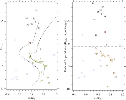
wherez=flux(i, j) are the flux count values for eachKepler pixel within the postage stamp. To generate positions from the optimal aperture, anyzvalue not in the optimal aperture is set to zero. To reduce the computational load and to smooth out high-frequency positional variations, normal points (NPs) are formed by averaging thexandypositions for a specified time span. The tests and results reported herein are based on nine day NPs. We also only use data within an optimal aperture for each star defined by theKeplerteam. We provide an example of an optimal aperture for a star withKepleridentification number KID=7031732 in Figure 3. There are positional corrections tabulated in the MAST data products, e.g., POS_CORR1. These corrections report the size of the differential velocity aberration, pointing drift, and thermal effects applicable to the region of sky recorded in the file. These corrections are applied to our derived centroids. The final positions used in the test are corrected using the MAST position correction values,
e.g., XY_CORR=MOM_CENTR_XY - POS_CORR_XY. We
calculate the standard deviation of each NP along each axis for each star. The average standard deviation of these NP is typically on the order of 1 mas, demonstrating exceptional astrometric stability within each postage stamp. However, this small, formal random error is a significant underestimation of the total star-to-star astrometric quality, as we will see below in Section4.1. We explored utilizing PSF fitting methods to extract positions. That approach did not resolve the issue of poor astrometric performance over multiple quarters (see Section 4.3 below). PSF fitting is computationally intensive and complicated given the KeplerFOV crowded stellar field and the significant PSF variations over that field (Bryson et al.2010).
4.KEPLERASTROMETRIC TESTS
These tests highlight several systematic errors and motivate our simple strategy for dealing with them. We employ GaussFit
Figure 3.Left: KID 7031732 in a crowded field. Image from Digital Sky Survey viaAladin. Middle: postage stamp for KID 7031732. Right: optimum aperture for KID 7031732.
[image:4.612.62.555.458.709.2]for all of our astrometric modeling (Jefferys et al. 1988) to minimizeχ2.
4.1. Single Channel, Single Season, Single Quarter
These tests use 95 stars located in Channel 21, Season 0, Quarter 10 that are identified as red giants in theKeplerInput Catalog (KIC). This initial filtering by star type potentially minimizes any effects of proper motion over the span of one or even two quarters. The NP generator, run on each star selected from test Channel 21, effectively reduces the number of discrete data sets per star from on the order of 4500 down to 9. We assign the 9 NPs for each of the 95 stars in the test to the 9 “plates.” Each plate now contains 95 stars whose epochs are separated in time by approximately 9 days. Using the positions and positional errors generated by the NP code (now organized as 9 “plates” each containing 95 star positions and associated errors), we determine scale, rotation, and offset “plate constants” relative to an arbitrarily adopted constraint epoch (the so-called “master plate”) for each observation set (the positions generated for each star within each “plate” at each of the nine NP epochs). The solved equations of condition are
ξ =Ax+By+C, (3)
η= −Bx+Ay+F, (4)
where x and y are the measured NP coordinates from the Kepler postage stamps. A and B are scale and rotation plate constants, C and F are offsets. For this test spanning only a single 90 day quarter, we ignore proper motions. When modeling these positions, in order to approach a near-unityχ2/ DOF (DOF=degrees of freedom), the input positional errors, standard deviations from the NP averaging process, had to be increased by a factor of four. The final catalog of (ξ, η) positions have averageσξ =0.31 millipixel andση =0.64 millipixel
(1.23 and 2.54 mas), which is seemingly quite encouraging if one’s goal is precision astrometry withKepler.
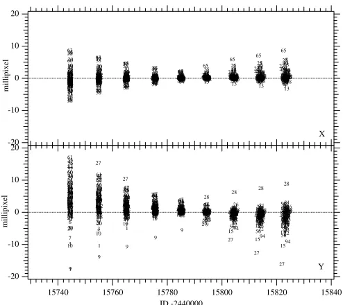
However, the results of this modeling, shown in Figure 4, exhibit large systematic effects that are well cor-related with time. The constraint epoch for this reduction is JD−24400000=15785.2, that is, the middle epoch of the nine plotted. We tentatively blame the typically largeryresiduals (yis larger thanxwithin each epoch) in Figure4with charge-transfer smearing along the CCD column readout direction (Kozhurina-Platais et al. 2008; Quintana et al. 2010). Our ultimate goal is to tease out stellar positional behavior similarly correlated with time: proper motion. We find stars 9 (=KID 6363534) and 27 (=KID 6606001) to exhibit some of the largest and most strikingly systematic residual patterns. Figure5provides an explanation for the behavior of star 27 (a close companion that perturbed the simple first-moment centering algorithm), and presents a puzzle regarding star 9. This star has no bright com-panions, yet it is a poorly behaved component of our astrometric reference frame. We suspect that this is due to the CCD channel-to-channel cross-talk discussed in Caldwell et al. (2010b). Four CCDs share common readout electronics. A bright star on one CCD can affect the measured charge in another.
To determine whether or not there might be unmodeled—but possibly correctable—systematic effects at the 10 millipixel level, we plotted the reference framexandyresiduals against a number of parameters. These included the following:x, y posi-tion within the channel; radial distance from the channel center; reference star magnitude and color; and epoch of observation.
-20 -10 0 10 20 millipixel 15840 15820 15800 15780 15760 15740 JD -2440000 1 2 3 4 5 6 7 8 9 10 11 12 13 14 151617
18 19 20 21 22 23 24 25 26 28 29 30 31 32 33 34 35 36 37 38 39 40 41 42 43 44 45 46 47 48 49 50 51 52 53 5455 56 57 58 59 60 61 62 63 64 65 66 67 68 69 70 71 72 73 74 75 76 77 78 79 80 81 82 83 84 85 86 87 88 89 90 91 92 93 94 95 96 97 1 2 3 4 5 6 7 8 9 10 1112 13 14 15 1617 18 19 20 21 22 23 24 25 26 27 28 29 30 31 32 33 34 35 36 37 38 39 40 41 42 43 44 45 46 47 48 49 50 51 52 53 5455 56 57 58 59 60 61 62 63 64 65 66 67 68 6970 71 72 73 74 75 76 77 7879 80 81 82 8384 85 8687 88 89 90 91 92 93 94 95 96 97 1 2 3 4 5 6 7 8 9 10 11121314 15 1617 18 19 20 21 22 23 24 25 26 27 28 29 30 31 32 33 34 35 36 37 38 39 40 41 42 43 44 45 46 47 48 49 50 51 52 53 5455 56 57 5859 60 61 62 63 64 65 66 6768 6970 71 72 73 74 75 76 77 7879 80 81 82 8384 85 8687 8889 9091 9293 94 95 96 97 1 2 354 6 7 8
9 10 11121314 151617 18 19 20 212322 24 25 26 27 28 293031 32 33 34 35 36 37 38 39 40 41 42 43 44 4546 47 48 49 50 51 52 53 5455 56 57 5859 60 61 62 63 64 6566 67 68 6970 71 72 73 74 75 76 77 7879 80 81 82 8384 85 8687 88 89 9091 929597939496 34256718
9 10 1112 1314 1516 171819 20 2123242522 26 27
28
293031 32 3334 35 36 37 38 39 40 41 42 4344 4546 47 48 49 50 51 52 53 5455 5658605759 61
62 63 64
65666768 6970 71 72 73 7475 7677 7879 80 81 82 83 84 85 868790928889919394
95 96 97 1 2 34 5 6 78 9 10 1112 13 14 15 1617201918 21 22 23 24 2526 27 28 2930 31 32 33353634 37 3840414239 4344 4546 47 48 49 50 5152 53 5455 56 57 5859 6061 62 63 64 65676866 6972707173 7475 7677 78 79 80 81 82 83 84 85 8687909288899193 94 95 96 97 1 2 3 4 5 6 7 8 9 10 1112 13 14 15 1617 18 19 20 21 22 23 24 25 26 27 28 29 30 31 32 33 34 35 36 37 384039 41 42 4344 4546 47 48 49 50 515253 5455
56 57 5859 6064616263 65676866 6971727073 74 757677 78 79 80 81 82 8384 85 8687908889 91 9293 94 95 96 97 1 2 3 4 5 6 7 8 9 10 11 12 13 14 15 1617 18 19 20 21 22 23 24 25 26 27 28 29 30 31 32 33 34 3536 37 384039
41 42 4344 45464748 49 50 5152 53 5455 56 57 5859 6061 62 63 64 65 66 67 68 6970 71 72 73 74
757677807879 81 82 8384 85 86 87908889
91 9293 94 95 96 97 1 2 3 4 5 6 7 8 9 10 11 12 13 14 15 1617 18 19 20 21 22 23 24 25 26 27 28 29 30 31 32 33 34 3536 3738 39 40 41 42 43 44 454647 48 49 50 5152 53 5455 56 57 5859 6061 62 63 64 65 66 6768 69 70 71 72 73 74
757776807879 81 82 8384 85 86 878889
90 91 9293 94 95 96 97 Y -20 -10 0 10 20 millipixel 1 2 3 45 6 7 8 9 10 11 12 13 14 1516 17 18 19 20 21 22 23 24 25 26 27 28 29 30 31 32 33 34 35 36 37 38 39 40 41 42 43 44 45 46 47 48 49 50 51 52 53 54 55 56 57 58 59 60 61 62 63 64 65 66 67 68 69 70 71 72 73 74 75 76 77 78 79 80 81 82 83 84 85 86 87 88 89 90 91 92 93 94 95 96 97 1 2 345 6 7 89 10 1112 13 14 15 16 17 18 19 20 21 22 23 24 25 26 2728 29 30 31 32 33 34 35 36 3738 39 40 41 42 43 44 45 46 47 485049 51 52 53 5455 56 57 58 59 60 61 62 63 64 65 66 67 68 69707172 73 74 75 76 77 7879 80 81 82 83 84 85 8687 88 89 90 91 92 93 94 95 96 97 2341
5 6789 10 11121314 15161718 19 20 2122 23 24 2526 2728 2930 31 32 3334 35 36 37 38 39 40 41 42 43 44 45 46 47 4849 5051 5253 5455 56 57 58 59 60 61 62 63 64 65 66 6768 697071 7273 74 7576777879 80 81 82 83 84 85 8687 88 89 9091 9293 94 95 96 97 11152116122510678133417202324518192221491
26 272928 30 31 32 3334 35 36 37 38 39 40 41 42 43 44 454748505152464953 5455 5657 58 59 60 61 62 63 64 6566 67 68 6970717273 74 7576777879 80 81 82 83 84 85 869092958889978796949391 151121161223201324103145617222798418191
25 26 272932333528303134 36 37 38 39 4041 42 4344 4551525446474849505553 56585759 6061 62 63 64 65 66 67 68 697470717275768373777880818279 84 85 868790928889979695939194 3457126
8 9 10 1112 13 14 15162117202223241918 25 26 27 28 2930 31 32 33353634 37 3840414239 4344 4556605158546362615764465250475949485553 65
66 67 68 697071 72 73 74757677818283787980 84 85 868790928889969791939495
1 2 34 5 6 7 8 9 10 1112 13 14 15162123241720221918 25
26 27
28 293031 32 33353634 37 3839 40 41 42 4344 45 46 47 48 49 50 515253 54
55 5657 58 59 6064616263 65
66 67 68 69717270 73 7475767783818284787980 85 868792939088978991959694
1 2 34 5 6 7 8 9 10 1112 13 14 15161718 19 20 21 22 23 24 25 26 27 28 293031 32 333534 36 37 3839 40 41 42 43 44 45 46 47 48 49 50 515253 5455 56 57 58 59 60616362 64 65
66 67 68 697071 72
73 74757677 78 79 80 81 82 8384 85 86 8790919288899395969794
1 2 34 5 6 7 8 9 10 11 12 13 14 15161718 19 20 21 22 23 24 25 26 27 28 293031 32 333435 36 373839 40 41 42 43 44 45 46 47 48 49 50 515253 54 55 56 57 58 59 6061 62 63 64 65 66 6768 69 70 71 72 73 747576 7778 79 80 81 82 8384 85
86 8788 89 9091 929396979495
[image:5.612.320.567.53.273.2]X
Figure 4.xandyresiduals as a function of time for the Q10-only four pa-rameter modeling from Section4.1. The residual clumps from left to right are “plates” 1–9, the epochs of the averaged normal points. Stars are labeled with a running number from 1 to 97. The residuals exhibit significant time depen-dency. Regarding two of the stars with more extreme behavior, neither star 9 (=KID 6363534) nor star 27 (=KID 6606001) is a high-proper-motion object.
We saw no obvious trends, other than an expected increase in positional uncertainty with reference star magnitude. Models with separate xandyscales (six parameters; in Equation (2) above, where−BandAare replaced byDandE) or color terms (eight parameters) provided no improvement inχ2/DOF.
Given that the pipelined positions available in the _llc.fits files are also first-moment centroids calculated from the opti-mal apertures, we developed the capability to generate these independently as a further test of the Kepler astrometry. The code used to generate the positions whose residuals are plotted in Figure4can also produce first-moment centroid data using the entire postage stamp (e.g., all the flux values in the mid-dle panel in Figure 3). By comparing the positions extracted from the entire postage stamp against the optimal subset of the postage stamp for Channel 21, the average absolute value residual is reduced by 30% when using the optimal apertures. However, tests carried out on Channel 41 (Season 0, Quarter 10) near theKeplerFOV center result in a much less significant improvement, only 12%. This can be explained by consider-ing the degradation in the PSF from the center to the edge of the entire Kepler FOV (Bryson et al.2010; Tenenbaum & Jenkins2010).
4.2. Other Single-channel Tests
4.2.1. Same Stars—Multiple Seasons and Quarters
Figure 5.Top: star 27 (POSS-J on the left, 2MASS on the right) obviously with a close companion that confused the first-moment centering. Bottom: star 9, similarly illustrated. No companion to star 9 is detected. The positional shift is assumed to be instrumental.
(A color version of this figure is available in the online journal.)
However, star 5 is relatively well behaved for any other season. A comparison of Figure6with Figure 5 in Barclay (2011)6is convincing evidence that astrometry quality and primary mirror temperature changes are correlated. Stable temperatures at any level yield better astrometry (smaller residuals).
4.2.2. An External Check of Single-channel, Single-season Data
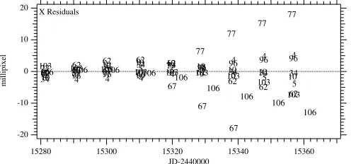
We carried out a four parameter modeling of 127 randomly chosen stars (a mix of dwarfs and giants according to the KIC) in Channel 26 from Season 3, Quarter 5 and found residual patterns similar to that for Season 3, Quarter 5, Channel 44 shown in Figure 6. We then extracted a subset of 10 stars, 5 with relatively well-behavedxresiduals (stars 4–62) and 5 with x residuals that are not constant with time (stars 67–106 in Figure7). We list these in Table2.
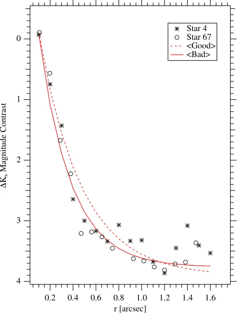
To explore the hypothesis that astrophysical effects (i.e., com-panions undetectable at the resolution of theKeplerdetectors) cause the observed residual behavior, these 10 stars were ob-served with the Keck NIRC2-AO system (Wizinowich et al. 2004; Johansson et al. 2008) on the nights of 2013 August
6 http://archive.stsci.edu/kepler/release_notes/release_notes12/DataRelease_
[image:6.612.317.569.508.641.2]12_2011113017.pdf
Table 2 Companion Test Stars
#a KID KEPMAG K FluxFracb
4 5698236 15.637 14.243 0.886
5 5698325 12.264 10.747 0.920
10 5698466 13.113 11.561 0.921
34 5783576 14.135 12.656 0.874
62 5784222 15.475 13.885 0.881
67 5784291 13.148 11.074 0.936
77 5869153 15.596 13.537 0.706
96 5869586 15.466 13.672 0.886
103 5869826 15.768 13.473 0.774
106 5870047 11.747 6.328 0.962
Notes.
aNumbering in Figure7.
bFraction of target flux in theKeplerproject-defined optimum aperture.
Figure 6.As in Figure4,xandyresiduals as a function of time for four parameter modeling of a sample of KIC-identified giants in Channels 41–44, but for 11 quarters. Top row, Quarters 3–6; middle row, Quarters 7–10; bottom row, Quarters 11–14. The top half of each box containsxresiduals withybelow. They-axis range within each coordinate half-box is±20 millipixels with anx-axis range between 80 and 90 days. The residuals exhibit time dependency within each quarter that correlates with focal plane temperature changes. Season 0 appears to have a larger fraction of stable astrometry.
-20 -10 0 10 20
millipixel
15360 15340
15320 15300
15280
JD-2440000
4
4
4
4 4 4 4 4
4 5
5 5
5
5 5 5 5 5 10
10 10 10
10 10 10
10
10 34 34
34 34 34
34 34 34
34 62
62 62
62 62
62
62 62
62 67
67 67
67 67
67 67
77
77
77
77
77
77
77 77
77
96 96 96
96
96 96 103 96 103 96 96
103 103 103
103
103 103
103 106 106
106
106 106
106 106
106
106
X Residuals
Figure 7.Selectedxresiduals as a function of time for four parameter modeling (Equations (3) and (4)) of 127 stars in Channel 26 from Season 3, Quarter 5. The star numbers are identified withKeplerIDs in Table2. Note that stars [4,. . ., 62] are more astrometrically stable than stars [67,. . ., 106].
2μm. The NIRC2 instrument was in the narrow field mode with a pixel scale of approximately 0.009942 pixel−1and a FOV of approximately 10.1 on a side. Each data set was collected with a three point dither pattern, avoiding the lower left quadrant of the NIRC2 array, with five images per dither position, each shifted
1from the previous. Each frame was dark subtracted and flat fielded. The sky frames were constructed for each target from the target frames themselves by median filtering and coadding the 15 dithered frames. Individual exposure times varied depending on the brightness of the target but were typically 10–30 s per frame. Data reduction was performed using a custom set of IDL routines.
[image:7.612.46.294.521.637.2]4 3 2 1 0 s Magnitude Contrast 1.6 1.4 1.2 1.0 0.8 0.6 0.4 0.2 r [arcsec] Star 4 Star 67 <Good> <Bad>
Figure 8.NormalizedK-band contrast curves for stars 4 and 67, along with average contrast curves for stars 4 through 62 (Good) and 67 through 106 (Bad). Note that while star 4 is more astrometrically stable than star 67, they have virtually identical contrast curves.
(A color version of this figure is available in the online journal.)
was above 0.5—a value determined with a “by eye” assessment. The location and flux of those PSFs that were detected were recorded over 5000 PSF plants. In each radius bin, the PSF with the smallest flux was used in the resulting plot of detected minimum magnitude difference (ΔKs) versus distance from the
science target.
We found no companion candidates in these images within a radius of 1.2. Figure 8 contains the contrast curves for star 4 (constant residuals) and star 67 (time-varying residuals), along with a fit to the normalized average contrast curves for stars 4–62 (Good) and 67–106 (Bad). To fit the average contrast curves, we employed an exponential function (y = K0 +K1∗exp(−(x−x0)/K2)) with offsetx0. The similarity of the average contrast curves removes small angular separation, fainter companions as the cause of the behavior displayed in Figure7. Finally, the average Season 3 crowding, contamination, and flux fraction parameters (see Fraquelli & Thompson2012 for parameter details) of the two groups differed little.
4.2.3. Lessons Learned
With as rich a data set as produced byKepler, our approach is to exercise extensive editing to establish the best astrometric reference frame: a reference frame with χ2/DOF ∼ 1 and Gaussian distribution of residuals. If we model only epochs 3–7 in Figure 4, as shown in Figure 9, we generate a final catalog of (ξ, η) positions with averageσξ = 0.22 millipixel
andση =0.46 millipixel (0.87 and 1.83 mas). The residuals
are Gaussian (Figure10) and naturally larger than the average
-20 -10 0 10 20 millipixel 15840 15820 15800 15780 15760 15740 JD -2440000 1 2 3 4 5 6 7 8 9 10 1112 13 14 15 1617 18 19 20 21 22 23 24 25 26 27 28 29 3031 32 33 34 35 36 37 38 39 40 41 42 43 44 4546 47 48 49 50 51 52 53 5455 56 57 5859 60 61 62 63 64 65 66 6768 6970 71 72 73 74 757677 7879 80 81 82 8384 85 8687 8889 9091 9293 94 95 96 97 1 2 34 5 6 7 8 9 10 11121314 151617 1819 20 21 22 23 24 25 26 27 28 29 3031 32 33 34 35 36 37383940 41 42 4344 454647 4849 50 51 52 53 5455 56 57 5859 60 61 62 63 64 65 66 67 68 69717270 73 747576777879 80 81 82 8384 85
868889909291939596979487 15274538698687372943561658601174424144407247525051675455576162636836652510121392902135858332753364818889777095966682847197765659342453281730203139344648492394939118142222680797873178199 1 2 3 4 56 789 10 11121314 151617 18 19 20 21 22 23 24 2526 27 28 29 30 31 32 33 34 35 36 37 38424339404144 45566962656058575464685251506367667071596146554947725348 73 747576778384857880818279 8687909288899193 94 95 96 97 1 2 3 4 5 6 7 8 9 10 11121314 15 1617 18 19 20 21 22 23 24 25 26 27 28 29 30 31 32 33 34 35 36 37 38 39 40 41 42 4344 454647 48 49 50 51 52 53 5455 56 57 5859 60 61 62 63 64 65 66 67 68 6970 71 72 73 74 75 76777879
80 81 82 8384 85 868790888991 9293 94 95 96 97 Y -20 -10 0 10 20 millipixel 1 2 34 5 6789 10 1112 13 14 1516211719201822 23 24 2526 272928 30 31 32 33 34 35 36 3738 39 40 41 42 43 44 45 46 47 4849 50 51 5253 5455 5657 58 59 60 61 62 63 64 65 66 6768 697274757071737677 7879 80 81 82 83 84 85 869092978889939596919487 151127242321252920161213103014171867895342622819221
31 32 33 34 35 36 3738 39 40 41 42 4344 454647485051524953 5455 56575859 60 61 62 63 64 65 66 67 68 6971727073 7475837677788081828479 85
868889909291939596978794 45152769607456433837298687581611645242441047755051724054555768676162636541859013363533213283129225979695348171898884767782177066465623242830313439204859495318782294789193261147328079199 15271611101221202324252834131417722259181986261 293031 32 33343536 37 3839 40 41 42 4344 4556505152545758464749554853 59 6061 62 63 64 65 66 67 68 6970717273 747576778384857880818279 868790928889979193959694
1 2 34 5 6 7 8 9 10 1112 13 14 15162117202223241918 25
26 27
28 293130 32 333534 36 37 3839 40 41 42 43 44 45 46 47 48 49 50 515253 54 55 56 57 58 59 606162 63 64 65 66 67 68 6970 71 72 73 747576 777879 80 81 82 8384 85 868790929388899697919594
X
Figure 9.xandyresiduals as a function of time for the Q10-only four parameter modeling from Section4.1. The residual clumps from left to right are “plates” 3–7, first seen in Figure4. Stars are labeled with a running number from 1 to 97. The residuals exhibit far less time dependency. Stars 9 and 27 continue to exhibit unmodeled behavior.
catalog errors because of the effective averaging to produce a catalog. Again, the significantly larger residuals along the y axis are likely due to CCD read-out issues (Kozhurina-Platais et al. 2008; Quintana et al.2010).
4.3. Two Channels, Two Contiguous Seasons
Again restricting our test to include only stars identified as red giants to minimize proper-motion effects, we now run a plate overlap model for the same set of stars appearing on two different Channels (21, 37) for Quarters 10 and 11, respectively. Given that the average absolute value UCAC4 proper motion for this suite of test stars is 7.5 mas yr−1(less than 2 millipixel yr−1), the roughly 180 day span of these data should exhibit very little scatter due to unmodeled motions. A four parameter model (with the constraint plate chosen to be from Channel 21) yielded a final catalog withσξ =2.60 millipixel andση =6.6 millipixel
(10.33 and 26.23 mas), which is significantly poorer astrometric performance than for a single channel and quarter (Section4.1). A six parameter model with separate scales alongxandyyielded only a 0.8% reduction in the large value of the reducedχ2/DOF. The Kepler telescope has a Schmidt–Cassegrain design. An effective astrometric model for such a telescope, used successfully in the past on Palomar Schmidt photographic plates, is introduced in Abbot et al. (1975) and used in, e.g., Benedict et al. (1978). That model,
ξ =Ax+By+Cxy+Dx2+Ey2
+F x(x2+y2) +G, (5)
η=Ax+By+Cxy+Dx2+Ey2
+Fy(x2+y2) +G, (6)
[image:8.612.47.294.57.381.2]200 150 100 50 0 Number
-4 -2 0 2 4
Residual (miillipixel) Y Residuals
= 0.8 millipixel N = 485
[image:9.612.58.280.52.441.2]200 150 100 50 0 Number X Residuals = 0.4 millipixel N = 485
Figure 10.Histograms ofxandyresiduals for the Q10-only four parameter modeling of only plates 3–7 (Figure9) from Section4.1. The residuals are well characterized with Gaussians with 1σdispersions as indicated.
than for Channel 21 alone. That the residuals remain large even with a Schmidt model demonstrates that the astrometric effects are not due to the Schmidt nature of the Kepler Telescope. The residuals as a function of position within the Channel 37 CCD show large variations on extremely small spatial scales (Figure12). We have yet to identify the source of these high-frequency spatial defects, but cannot yet rule out the individual field flatteners atop each module containing four channels (Tenenbaum & Jenkins 2010). This inter-channel behavior effectively prohibits the measurement of precise parallaxes using onlyKeplerdata.
5. ASTROMETRY OF AKEPLERTEST FIELD
Our ultimate goal is to produce an RPM diagram including KOIs, which would permit an estimate of their luminosity class. This may be feasible by restricting astrometry to a single channel and season. Essentially, we may be able to ignore the deficiencies demonstrated in Figures11and12because each star in any given season will be observed by the same pixels, and the starlight is passing through the exact same region of the field flattener. The 17 available quarters provide 3–4 same-season observation sets for anyKeplerchannel. Examination of Figure6supports our identification of Season 0 as one of the more stable. Tests similar to those carried out in Section 4.1
-100 -50 0 50 100 millipixel 15920 15900 15880 15860 15840 15820 15800 15780 15760 JD -2440000
1 1 1 1 1 1 1 1
1 1
2 2 2 2 2
2 2 2 2
2
4 4 4 4 4
4 4 4 4 4
5 5 5 5 5 5 5 5 5 5
6 6 6 6 6 6 6 6 6
6
7 7 7 7 7
7 7 7 7 7
9 9 9 9 9 9 9 9 9 9
10 10 10 10 10
10 10
10 10 10
11 11 11 11 11
11 11 11 11 11
12 12 12 12 12 12 12 12 12
12 13 13 13 13 13
13 13 13 13 13 14 14 14 14 14
14 14 14 14
14 15 15 15 15 15
15 15 15
15 15 16 16 16 16 16
16 16 16 16 16 17 17 17 17 17
17
17 17 17 17 18 18 18 18 18
18 18 18 18 18
19 19 19 19 19 19 19 19 19
19 21 21 21 21 21
21 21 21 21 21 22 22 22 22 22
22 22 22 22
22
23 23 23 23 23
23 23 23 23 23 24 24 24 24 24
24 24 24
24 24 25 25 25 25 25
25
25 25 25 25 26 26 26 26 26
26 26 26 26 26 27 27
27 27 27
27 27 27 27 27 28 28 28 28 28
28 28 28 28 28
29 29 29 29 29
29 29 29 29 29 3031 3031 3031 3031 3130 30 30 30 30 30
31 31 31 31
31 32 32 32 32 32
32 32 32
32 32 33 33 33 33 33
33 33 33
33 33 34 34 34 34 34
34 34 34 34
34 36 36 36 36 36
36 36 36 36 36 37 37 37 37 37
37 37 37 37 37
39 39 39 39 39
39 39 39
39 39
40 40 40 40 40 40
40 40 40
40 41 41 41 41 41
41
41 41 41
41 42 42 42 42 42
42 42 42
42 42 46 46 46 46 46
46 46 46 46
46 47 47 47 47 47
47
47 47 47 47 48 48 48 48 48
48 48 48 48 48 49 49 49 49 49
49 49 49 49 49
50 50 50 50 50 50 50 50 50 50
51 51 51 51 51 51 51 51 51 51
52 52 52 52 52
52 52 52 52 52 53 53 53 53 53
53 53 53
53
53 55 55 55 55 55
55 55 55
55
55 56 56 56 56 56
56 56 56
56
56
57 57 57 57 57 57
57 57 57
57 58 58 58 58 58
58 58 58
58 58 59 59 59 59 59
59 59 59
59 59 60 60 60 60 60
60 60 60
60 60 62 62 62 62 62
62 62 62 62
62
63 63 63 63 63 63 63 63 63
63 65 65 65 65 65
65 65 65
65
65
68 68 68 68 68 68 68 68 68
68 70 70 70 70 70
70
70 70 70
70 71 71 71 71 71
71 71 71 71
71
73 73 73 73 73
73 73 73
73 73 74 74 74 74 74
74 74
74 74
74 75 75 75 75 75
75 75 75 75
75
76 76 76 76 76 76 76 76 76
76
77 77 77 77 77 77 77
77 77
77
78 78 78 78 78 78 78
78 78
78
79 79 79 79 79 79 79 79 79
79 80 80 80 80 80
80 80 80 80
80 81 81 81 81 81
81 81 81
81
81 82 82 82 82 82
82 82 82
82
82 83 83 83 83 83
83 83 83
83 83 84 84 84 84 84
84 84 84 84
84 85 85 85 85 85
85 85 85
85
85 86 86 86 86 86
86 86 86
86 86
87 87 87 87 87
87 87 87 87
87 88 88 88 88 88
88 88 88 88 88
89 89 89 89 89
89 89 89 89
89
90 90 90 90 90
90 90 90 90
90 91 91 91 91 91
91 91 91 91 91 92 92 92 92 92
92
92 92 92 92 93 93 93 93 93
93 93 93 93 93 94 94 94 94 94
94 94 94 94 94 95 95 95 95 95
95 95 95 95 95
96 96 96 96 96 96 96 96 96
96 97 97 97 97 97
97 97 97 97 97 Y -100 -50 0 50 100 millipixel
1 1 1 1 1 1 1
1 1
1
2 2 2 2 2
2 2 2 2
2
4 4 4 4 4
4 4 4 4
4
5 5 5 5 5
5 5 5 5
5
6 6 6 6 6
6 6 6 6
6
7 7 7 7 7
7 7 7 7
7
9 9 9 9 9
9 9 9 9
9 10 10 10 10 10
10 10 10 10 10 11 11 11 11 11
11 11 11 11 11 12 12 12 12 12
12 12 12 12 12 13 13 13 13 13
13 13 13 13
13 14 14 14 14 14
14 14 14 14
14
15 15 15 15 15
15 15 15 15 15
16 16 16 16 16 16
16 16 16
16 17 17 17 17 17
17 17 17 17 17
18 18 18 18 18 18 18 18
18 18
19 19 19 19 19 19
19 19 19
19 21 21 21 21
21
21 21 21
21 21
22 22 22 22 22
22 22 22 22 22
23 23 23 23 23
23 23 23 23 23
24 24 24 24 24 24 24 24
24 24 25 25 25 25 25
25 25 25 25
25 26 26 26 26 26
26 26 26 26 26
27 27 27 27 27 27 27 27
27 27 28 28 28 28 28
28 28 28 28 28
29 29 29 29 29
29 29 29 29 29 30 30 30
30 30
30 30 30 30 30 31 31 31 31 31
31 31 31 31
31
32 32 32 32 32 32 32 32
32 32 33 33 33 33 33
33 33 33 33 33 34 34 34 34 34
34 34 34 34
34 36 36 36 36
36
36 36 36 36 36 37 37 37
37 37
37 37 37
37 37 39 39 39 39 39
39 39 39 39
39 40 40 40 40 40
40 40 40 40
40 41 41 41 41 41
41 41 41 41 41
42 42 42 42 42
42 42 42 42 42
46 46 46 46 46
46 46 46 46 46
47 47 47 47 47 47 47 47 47 47
48 48 48 48 48
48 48 48 48 48
49 49 49 49 49
49 49 49 49 49
50 50 50 50 50
50 50 50 50 50 51 51 51 51 51
51 51 51 51
51 52 52 52 52 52
52 52 52 52 52 53 53 53 53 53
53 53 53
53
53
55 55 55 55 55
55 55 55 55
55
56 56 56 56 56 56 56 56
56 56 57 57 57 57 57
57 57 57 57 57
58 58 58 58 58 58 58 58 58
58 59 59 59 59 59
59 59 59 59 59
60 60 60 60 60
60 60 60 60 60 62 62 62 62 62
62
62 62 62 62 63 63 63 63 63
63 63 63 63 63 65 65 65 65 65
65 65 65
65
65 68 68 68 68 68
68 68 68 68
68 70 70 70 70 70
70 70 70 70 70 71 71 71 71 71
71 71 71 71 71
73 73 73 73 73
73 73 73 73 73
74 74 74 74 74 74
74 74 74 74 75 75 75 75 75
75
75 75 75 75 76 76 76 76 76
76
76 76 76 76 77 77 77 77 77
77 77 77 77 77 78 78 78 78 78
78 78 78 78 78
79 79 79 79 79
79 79 79
79
79
80 80 80 80 80
80 80 80 80 80 81 81 81 81 81
81 81 81 81 81 82 82 82 82 82
82 82 82 82 82 83 83 83 83 83
83
83 83 83 83 84 84 84 84 84
84
84 84 84 84 85 85 85 85 85
85 85 85 85
85 86 86 86 86 86
86 86 86 86 86
87 87 87 87 87
87 87
87 87 87 88 88 88 88 88
88
88 88 88 88 89 89 89 89 89
89 89 89 89 89 90 90 90 90 90
90
90 90 90 90 91 91 91 91 91
91 91 91 91 91
92 92 92 92 92 92
92 92 92
92 93 93 93 93 93
93 93 93 93 93 94 94 94 94 94
94 94 94 94
94 95 95 95 95 95
95 95 95 95
95 96 96 96 96 96
96 96 96 96
96 97 97 97 97 97
97 97 97 97
97
[image:9.612.322.567.54.269.2]X
Figure 11.xandyresiduals in millipixels as a function of time from the full Schmidt 14 parameter modeling from Section4.3. The residual clumps on the left-hand side (Channel 21) from left to right are “plates” 3–7. Stars are labeled with a running number from 1 to 97. Note the scale change along they-axis, a range five times larger than that in Figure9. The residuals exhibit extreme time dependence. Star 27 continues to show unmodeled behavior in both channels. Virtually all stars in Channel 37 (right) exhibit unmodeled behavior.
-600 -400 -200 0 200 400 600
CCD row [pixel]
-600 -400 -200 0 200 400 600
CCD column [pixel]
1 2 4 56 7 9 10 11 12 13 14 15 1617 18 19 21 22 23 2425
26 2728 29 30 31 32 33 34 36 37 3940 41 42 46 47 48 49
505152
53 55 56 57 5859 60 62 63 65 68 70 71 73 74 75 76 77 78
79 8081 82 8384 85 86 87 88 89 90 91 92 93 94 95 96 97 100 mas
Figure 12.Average vector residuals in milliarcseconds (scale at lower left) as a function of position within Channel 37 from the full Schmidt 14 parameter modeling of Channel 21 and Channel 37 described in Section4.3. All positions have been re-origined to the CCD center. Note the extreme variation in vector length and position angle over small spatial scales, for example, the grouping consisting of stars 22 through 34 (row∼50, column∼−200). Comparing Channel 21 with Channel 37 demonstrates serious astrometric systematics on very small spatial scales.
yielded very poor results for Quarter 2, and hence it is unused here.
5.1. Populating an RPM Diagram
[image:9.612.322.567.342.586.2]stars with 14>KEPMAG>11.6 (Quarters 6, 10, and 14, and all Season 0):
1. Approximately 100 stars classified as red giants; 2. Approximately 100 stars withTeff>6500 K; 3. Approximately 100 stars with 6200>Teff>5100 K; 4. Approximately 30 stars withTeff <5000 K and Total_PM
0.24yr−1with any KEPMAG value; and
5. All KOIs found in Channel 21, e.g.,Planetary_candidate andExoplanet_host_starcondition flag objects. These also have unrestricted KEPMAG.
We extract positions and generate nine day average NPs using only theKepler team defined optimal apertures for each star. When including these data in our modeling with the ground-based catalogs, we re-origin theKeplerx, y coordinate values to (0,0) at the center of Channel 21.
5.2. Reference Star Priors
To place our relative astrometry onto a right ascension (R.A.), declination (decl.) system, we extract J2000 positions and proper motions from the UCAC4 (Zacharias et al.2013) and PPMXL (Roeser et al. 2010) catalogs. The catalog positions scale the Kepler astrometry and provide an approximately 12 yr baseline for proper-motion determination. Additionally, the catalog proper motions with associated errors are entered into the modeling as quasi-Bayesian priors. These values are not entered as hardwired quantities known to infinite precision. Theχ2minimization is allowed to adjust the parameter values suggested by these data values within limits defined by the data input errors.
The input positional errors average 19 mas for the UCAC4 and 63 mas for the PPMXL. The average per-axis proper-motion errors are 2.6 mas yr−1 for UCAC4 and 3.9 mas yr−1 for PPMXL. A comparison of the two catalogs yields an average per-star absolute value proper-motion disagreement of 5.1 mas yr−1, indicating that there is room for improvement. The R.A. and decl. positions from the two catalogs are used to calculateξ, ηstandard coordinates transformed from radians to arcseconds (van de Kamp1967) using the center of Channel 21 as the tangent point.
5.3. The Proper-motion Astrometric Model
Using the central five epochs of positions from Quarters 6, 10, and 14 fromKeplerChannel 21 (the editing of each quarter can be illustrated by comparing Figure4to Figure9), spanning 2.14 yr, with standard coordinates from PPMXL and UCAC4, and proper-motion priors from the latter two catalogs, we determine “plate constants” relative to the UCAC4 catalog (this catalog having smaller formal positional errors). The constraint epoch is thus 2000.0. Our reference frame after pruning out astrometrically misbehaving objects contains 226 stars. For this model, we include only those stars with a restricted magnitude range, 14 > KEPMAG > 11.6 (samples 1–3 discussed in Section5.1above). The average magnitude for this magnitude-selected reference frame isKEPMAG =13.3.
Again, we employ GaussFit (Jefferys et al.1988) to minimize χ2. The solved condition equations for the Channel 21 field are now
ξ =Ax+By+Cxy+Dx2+Ey2
+F x(x2+y2) +G−μxΔt, (7)
η=Ax+By+Cxy+Dx2+Ey2
+Fy(x2+y2) +G−μyΔt, (8)
where x = x−500 and y = y−500 are the re-origined measured coordinates fromKeplerand the standard coordinates from UCAC4 and PPMXL;μx andμyare proper motions; and Δtis the epoch difference from the mean epoch.
Based on the resulting astrometric parameters, we form a plate scale of
S=(BA−AB)1/2, (9) and for the 15 epochs (five for each of the three quarters) of Keplerobservations find S =3.97664 ±0.000009 pixel−1, which is close to the nominalKeplerplate scale (van Cleve & Caldwell2009) and an indication that theKeplertelescope plate scale as sampled in Channel 21 was quite constant. The scale factor of the PPMXL catalog relative to the UCAC4 catalog was 1.000012.
5.4. Assessing the Reference Frame
Using the UCAC4 catalog as the constraint plate to achieve a χ2/DOF ∼ 1, the Kepler NP data errors (NP standard deviations) had to be increased by a factor of 16. Histograms of theKeplerNP residuals were characterized byσx =3.6 mas,
σy =6.4 mas. The average absolute value residual forKepler
was 4.8 mas, 24.3 mas for UCAC4, and 61.6 mas for PPMXL. The resulting 226 star reference frame “catalog” in ξ and η standard coordinates was determined with average positional errors of σξ,η = 8.6 mas, a 55% improvement in relative
position over the UCAC4 catalog. The average proper-motion error for the stars comprising the reference frame is 0.8 mas yr−1. Again, to determine whether or not there might be unmodeled—but possibly correctable—systematic effects, we plotted the reference framexandyresiduals against a number of parameters. These included thex, yposition within the chan-nel (Figure13), the radial distance from the channel center, the reference star magnitude and color, and the epoch of observa-tion. We saw no obvious trends other than an expected increase in positional uncertainty with reference star magnitude. Plots ofxandyresidual versus pixel phase also indicated no trends. We calculate the pixel phase,φx =x−int(x+ 0.5), whereint
returns the integer part of the (for example)xcoordinate.
5.5. Applying the Reference Frame
To ensure that the typically fainter (and hence less valuable contributors to the astrometric reference frame) stars do not affect our astrometric modeling of the Channel 21 CCD, an identical model in Section 5.3is re-run, adding NP positions for the K and M stars (sample 4) and KOIs (sample 5) from Section5.1, holding the Equations (7) and (8) coefficientsA–G to the values determined in Section5.3. Note that we do solve for the positions and proper motions. This yields final catalog positions and proper motions for 301 stars representing all the categories listed in Section 5.1. The inclusion of fainter stars results in a “catalog” withξandηstandard coordinates average relative positional errors σξ,η = 11.1 mas, and an average
600
400
200
0
-200
-400
Y
(pixel)
600 400
200 0
-200 -400
[image:11.612.320.569.49.252.2]X (pixel) 5 mas
Figure 13.Average vector residuals in milliarcseconds as a function of position within Channel 21 from the full Schmidt 14 parameter modeling of three Season 0 observation sets described in Section5.3. Other than a strong tendency for larger residuals in the y direction, the pattern is satisfactorily random.
have lower signal to noise and, if included, would degrade our astrometric reference frame.
We present final KOI proper motions and errors in Table 3. These are, in a sense, absolute proper motions be-cause of the use of prior information. To reiterate, we treated the UCAC4 and PPMXL proper-motion priors as observations with corresponding errors. The Table 3 KOI proper-motion parameters (and those for the entire set of reference stars modeled above) were adjusted by various amounts depend-ing on the data input errors to arrive at a final result that minimizedχ2.
5.6. Reference Star Photometric Stability
Our NP generation process (Section3.2) also produces an av-erage magnitude. In the case of nine day NPs, all of the measured flux values in each optimum aperture are averaged over the nine day interval and converted to a magnitude with an arbitrary zero point throughmf =25.768–2.5∗log10(flux). Because we
re-stricted this test to a single channel, no background correction is applied. The standard deviation for the 15 averagemf
magni-tudes is plotted against reference star ID number in Figure14. Referencing Section5.1, stars 1–99 are classified as red giants in the KIC (sample 1), stars 100–199 are hotter stars (sample 2), stars 201–299 are intermediate temperature stars (sample 3), stars 300–350 are selected to be more likely K and M dwarfs (sample 4), and stars 400–452 are the KOIs found in Channel 21 (sample 5). Note that all ID numbers are not present in the plot due to the editing process (Section5.3) that produces the final astrometric reference frame.
The highest maximum variability with a nine day cadence is found in our sample of suspected giants, which was not an unexpected result (Bastien et al. 2013). The KOIs seem to have photometric variability characteristics most similar to the K, M group. We note trends toward smaller variation with increasing number within each group (as defined in Section5.1). This may be a function of photometric noise characteristics
Figure 14.Measured photometric dispersion (mf standard deviation) over 2.1
ywith a nine day cadence for each star modeled in Section5.3. Giants (1–100) exhibit the highest overall variability. Other groups are the hot star sample (101–199), mid-rangeTeff (201–299), the K–M star sample (300–350), and
the KOI sample (400–452). The trends to smaller photometric variation with number within each sample group (as defined in Section5.1) may be a function of position within Channel 21. The lowest variations are closer (x, y)=(0, 1000) while the highest are closer (x, y)=(1000, 0).
having positional dependence within Channel 21. The selection process populating each group and allocating a running number within each group always assigned the lowest numbers closer to (x, y)=(0, 1000) and the highest closer to (x, y)=(1000,0).
5.7. Astrometry as a Diagnostic
Figure15contains an average absolute valueKepler xresidual for each reference star and KOI (numbering from Table3) as a function ofmf. The residuals are calculated from the Section5.3
modeling results. We choose the x residual as a potential diagnostic given that theyresiduals are generally systematically larger (see Figures10and13). The trend line is a quadratic fit to thexresiduals for the reference stars only (samples 1–3 in Section5.1). The planet-hosting KOIs over-plotted with large font show no extreme astrometric behavior, all lying within
±3σof the relation. However, several KOI hosting unconfirmed planetary companions exhibit astrometric peculiarities. Both KOI 426 and 452 were inspected in 2MASS and Palomar Sky Survey images and showed no nearby stellar companions or image structure indicative of close stellar companions. In addition, KOI 452 is the most photometrically variable (Figure14) host candidate star. Unfortunately, given the random eruption of astrometric peculiarity (see Figure 5), astrometry alone cannot serve as a reliable indicator of astrophysically interesting behavior.
5.8. RPM Diagrams: Pre- and Post-Kepler
We now have the proper motions required to generateHK(0)
values for an RPM (Section 2). K-band magnitudes, J − K colors, and interstellar extinction values,AV,E(B−V), were
extracted from the onlineKeplertarget database at MAST. We assumed (Schlegel et al.1998) extinction-corrected byK(0)= K − AK and (J −K)0 = (J −K)−E(J−K), with AK =
AV/9 andE(J −K)=0.53*E(B−V). The left-hand RPM in
[image:11.612.48.295.56.296.2]Table 3
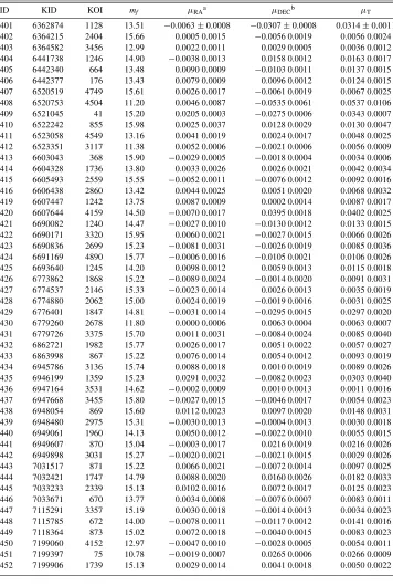
Channel 21 KOI Proper Motions (μ)
ID KID KOI mf μRAa μDECb μT
401 6362874 1128 13.51 −0.0063±0.0008 −0.0307±0.0008 0.0314±0.0011
402 6364215 2404 15.66 0.0005 0.0015 −0.0056 0.0019 0.0056 0.0024
403 6364582 3456 12.99 0.0022 0.0011 0.0029 0.0005 0.0036 0.0012
404 6441738 1246 14.90 −0.0038 0.0013 0.0158 0.0012 0.0163 0.0017
405 6442340 664 13.48 0.0090 0.0009 −0.0103 0.0011 0.0137 0.0015
406 6442377 176 13.43 0.0079 0.0009 0.0096 0.0012 0.0124 0.0015
407 6520519 4749 15.61 0.0026 0.0017 −0.0061 0.0019 0.0067 0.0025
408 6520753 4504 11.20 0.0046 0.0087 −0.0535 0.0061 0.0537 0.0106
409 6521045 41 15.20 0.0205 0.0003 −0.0275 0.0006 0.0343 0.0007
410 6522242 855 15.98 0.0025 0.0037 0.0128 0.0029 0.0130 0.0047
411 6523058 4549 13.16 0.0041 0.0019 0.0024 0.0017 0.0048 0.0025
412 6523351 3117 11.38 0.0052 0.0006 −0.0021 0.0006 0.0056 0.0009
413 6603043 368 15.90 −0.0029 0.0005 −0.0018 0.0004 0.0034 0.0006
414 6604328 1736 13.80 0.0033 0.0026 0.0026 0.0021 0.0042 0.0034
415 6605493 2559 15.55 −0.0052 0.0011 −0.0076 0.0012 0.0092 0.0016
416 6606438 2860 13.42 0.0044 0.0025 0.0051 0.0020 0.0068 0.0032
419 6607447 1242 13.75 0.0087 0.0009 0.0002 0.0014 0.0087 0.0017
420 6607644 4159 14.50 −0.0070 0.0017 0.0395 0.0018 0.0402 0.0025
421 6690082 1240 14.47 −0.0027 0.0010 −0.0130 0.0012 0.0133 0.0015
422 6690171 3320 15.95 0.0060 0.0021 −0.0027 0.0015 0.0066 0.0026
423 6690836 2699 15.23 −0.0081 0.0031 −0.0026 0.0019 0.0085 0.0036 424 6691169 4890 15.77 −0.0006 0.0016 −0.0105 0.0021 0.0106 0.0026
425 6693640 1245 14.20 0.0098 0.0012 0.0059 0.0013 0.0115 0.0018
426 6773862 1868 15.22 −0.0089 0.0024 −0.0014 0.0020 0.0091 0.0031
427 6774537 2146 15.33 −0.0023 0.0014 0.0026 0.0013 0.0035 0.0019
428 6774880 2062 15.00 0.0024 0.0019 −0.0019 0.0016 0.0031 0.0025
429 6776401 1847 14.81 −0.0031 0.0014 −0.0295 0.0015 0.0297 0.0020
430 6779260 2678 11.80 0.0000 0.0006 0.0063 0.0004 0.0063 0.0007
431 6779726 3375 15.70 0.0011 0.0031 −0.0084 0.0024 0.0085 0.0040
432 6862721 1982 15.77 0.0026 0.0017 0.0051 0.0022 0.0057 0.0027
433 6863998 867 15.22 0.0076 0.0014 0.0054 0.0012 0.0093 0.0019
434 6945786 3136 15.74 0.0088 0.0018 0.0010 0.0019 0.0089 0.0026
435 6946199 1359 15.23 0.0291 0.0032 −0.0082 0.0023 0.0303 0.0040
436 6947164 3531 14.62 −0.0002 0.0009 0.0010 0.0013 0.0011 0.0016
437 6947668 3455 15.80 −0.0027 0.0015 −0.0046 0.0017 0.0054 0.0023
438 6948054 869 15.60 0.0112 0.0023 0.0097 0.0020 0.0148 0.0031
439 6948480 2975 15.31 −0.0030 0.0013 −0.0004 0.0013 0.0030 0.0018
440 6949061 1960 14.13 0.0050 0.0012 −0.0022 0.0010 0.0055 0.0015
441 6949607 870 15.04 −0.0003 0.0017 0.0216 0.0019 0.0216 0.0026
442 6949898 3031 15.27 −0.0020 0.0021 −0.0021 0.0015 0.0029 0.0026
443 7031517 871 15.22 0.0066 0.0021 −0.0072 0.0014 0.0097 0.0025
444 7032421 1747 14.79 0.0088 0.0020 0.0160 0.0026 0.0182 0.0033
445 7033233 2339 15.13 0.0102 0.0016 0.0072 0.0017 0.0125 0.0023
446 7033671 670 13.77 0.0034 0.0008 −0.0076 0.0007 0.0083 0.0011
447 7115291 3357 15.19 0.0030 0.0018 −0.0014 0.0013 0.0034 0.0023
448 7115785 672 14.00 −0.0078 0.0011 −0.0117 0.0012 0.0141 0.0016
449 7118364 873 15.02 0.0072 0.0018 −0.0040 0.0015 0.0083 0.0023
450 7199060 4152 12.97 −0.0047 0.0010 −0.0028 0.0005 0.0054 0.0011
451 7199397 75 10.78 −0.0019 0.0007 0.0265 0.0006 0.0266 0.0009
452 7199906 1739 15.13 0.0029 0.0014 0.0041 0.0018 0.0050 0.0022
Notes.
aProper motions in arcseconds per year. bCorrected for cosδdeclination.
main sequence and an ascending sub-giant branch. The average HK(0) error is 0.43 mag, but is dependent on the value ofμvec with an increased error toward bright values ofHK(0).
The scatter in the left of Figure 16 can be due to several causes. These causes include proper-motion accuracy, random motions of stars, and systematic motions of stars. TheHK(0)
average error bar in the figure indicates a±0.4 mag of scatter due to measurement errors. The amount due to random stellar motions is unknown. Any particular star could have a large radial component to its random motion and be erroneously
placed among the giant stars with typically lower than average proper motions. Those two effects increase the random scatter in an RPM. That systematic motions can corrupt an RPM is illustrated in Benedict et al.’s (2011) Figure 3. There, the RR Lyr variables all lie below and blueward of the broad main sequence. These Pop II giant stars have anomalously large proper motions, causing their erroneous placement in the RPM.