I
11111~
I7.
Factors influencing water temperature on farms and the effect
of warm drinking water on pig growth
I T. Banhazil and D. Rutley2
1Natianal Centre far Engineering in Agriculture (NCEA), University afSauthern Queensland, West Street, Taawaamba, QLD 4530, Australia; 2Uvestack Systems Alliance, The University af Adelaide, Rasewarthy Campus, SA 5371, Australia; thamas.banhazi@usq.edu.au
Abstract
Drinking water temperature was measured continuously for one year on 22 pig farms in South Australia (SA) and Queensland (QLD) and data were collected on major housing features and management factors employed in individual piggery buildings. The data collected enabled the likely effects of housing and management factors on resulting water temperature to be quantified and the industry to be made aware of the importance of providing drinking water within temperature range for efficient pig production and welfare. The data collected identified statistically significant housing and management factors associated with and contributing to sub optimal water temperature as seasons (P=O.OOO1), source of water (P=O.OOO1), position of piping (P=0.003), water pressure (P=O.042), size ofin-shed water reservoir (P=0.0001) and diameter of the main (P=O.OOO 1) and delivery pipes (P =0.000 1). A controlled experiment was also conducted to complement these findings by quantifying the negative effect of sub-optimal (warm) drinking water temperature on pig growth rate. Two identical weaner rooms were selected for the on farm study. Genetics, nutrition, management, stocking rate and density were identical for both groups. Pigs in the treatment group received water heated to 28.3±OA °C while the control group received unheated water at 17.8±0.9
dc.
Growth rate was suppressed by 58 grams/day in the group receiving the heated water. These results demonstrate the negative effect of warm water temperature on pig production and highlight potential ways of reducing the likelihood of providing warm drinking water to livestock.Keywords: management, drinking water, thermal environment, temperature, growth rate
7.1 Introduction
The thermal environment of intensively housed pigs is predominantly influenced by air temperature, humidity and airspeed (Black et al., 2001; Jones and Nicol, 1998; Le Dividich and Herpin, 1994; Zhang et a/., 1992). However, other factors such as the temperature of drinking water can also have a significant effect on how individual animals will be affected by the thermal conditions in the sheds (Brooks and Carpenter, 1990). It was hypothesised that warmer drinking water will discourage animals from drinking adequate water, in turn reducing their feed intake (Morrison et al., 2007; Yang et al., 1984) and growth. While no firm drinking water temperature recommendations exist for pigs, some studies suggest that 'cool drinking water may improve feed intake. Although, studies (Bigelow and Houpt, 1988; Van der Peet-Schwering et al., 1997)
indicate that water temperature might have a significant effect on water intake in pigs, the overall
A. Aland and 1, Banhazi (eds.) Livestock housing: modern management to health and welfare of farm animals 147 DOll 0.3920/978-90-8686-771-4_07, © Wageningen Academic Publishers 2013
-~"'--1III
""I
T. Banhazi and D. Rutley
effect of drinking water temperature on pig production has not been assessed under Australian farming conditions. ,
Therefore, this study was designed with a number of aims in mind. First, information on drinking water temperature and factors potentially influencing drinking water temperature were collected during the survey component of the project. This information enabled the research team to document the extent of sub-optimal drinking water temperature present in piggery buildings and to identify relationships between features of watering systems and drinking water temperature. Such information is not available in the literature currently. In addition a related on-farm experiment was designed to quantify production loss associated with sub-optimal drinking water temperature. Overall the study enabled researchers to develop strategies to optimise drinking water temperature for pigs in summer and winter by identifying practical ways of improving the thermal control of watering systems in commercial piggeries. As a result, it was hoped that the production efficiency'and welfare of pigs could be improved.
7.2 Materials and methods
7.2.1 Study farms
Twenty-two farms were selected for the survey with 10 in Queensland (QLD) and 12 in South Australia (SA). On each farm, water temperature was monitored continuously for 12 months in one of the 4 buildings selected within the same farm. Farms in SA were located in the Northern, Central and Riverland regions to represent Mediterranean, cold temperate and warm temperate zones found in Western Australia, Victoria and Southern New South Wales (NSW). Farms in QLD were selected in the sub-tropical region representative of the northern NSW and Southern and Central QLD. The study sheds included a wide range of design and management options and sites were chosen to provide a representative sample of industry practice in Australia.
7.2.2 Measurement methods and location
Temperature data were recorded in all study buildings using Tinytalk temperature loggers (Tinytalk-2, Hastings Data loggers Pty. Ltd., Port Macquarie, Australia). These self-contained and battery-powered data loggers with external sensors on a lead have the capacity to record temperature and humidity data for up to one year, depending on the pre-set logging interval (Banhazi et al., 2008). A 72 minute logging interval was selected and standardised for the whole project, allowing the data loggers to run unattended for ninety days (3 months, a whole season), The choice of a 72-minute interval was a good compromise between obtaining an accurate environmental record and producing excessive redundant data. The external temperature leads of the sensors were inserted in the water pipes as close to the drinkers as practically possible, without allOwing the pigs to interfere with the instruments. Care was taken to ensure the installed sensors did not impinge on the normal operation and management of the piggery.
148 Livestock housing
7. ~atertemperature on farms and the effect of warm drinking water on pig growth
7.2.3 On-farm experiment
Two identical weaner rooms were selected for the second study. Genetics, nutrition and management were identical for both groups. Pigs were included in the experiment from weaning until approximately 25 kg or 10 weeks of age. Stocking rate was similar for both groups, the control group consisted of 93 pigs and the trial group consisted of 82 pigs. Pigs in the treatment group received water heated to 28.3±OA °C while the control group received drinking water managed according to normal management practices without any heating or cooling (untreated) at 17.8±O.9
0c.
Large-capacity commercial aquarium heaters were used to heat the water in the water reservoir to the pre-set temperature (Fluval Aquarium Heater, Hagen Inc. Montreal, Canada). The temperature of the heated water was based on the preliminary analysis of field measurements and was the upper quartile of the summer water temperatures recorded on South Australian farms. Heaters were evaluated first under laboratory conditions, using a large water tank of identical size to the water tanks used for the subsequent on -farm trial. Growth rate was monitored in both the experimental and control groups using an electronic scale (Weigh Crate, Ruddweigh, Guyra, Australia).7.2.4 Data handling
A questionnaire was developed to collect information relating to the engineering features and setup ofthe watering systems used in individual buildings. Each farm received four one-day visits, corresponding with the four seasons. At each quarterly farm visit the data was extracted from the loggers and downloaded to a portable computer on site. The extracted data. and the sensors were inspected during these visits to ensure the proper functioning of the loggers throughout the data collection period. For each logging site a form was filled out to record all installation details. After downloading, the data files were named using a standardised system, which enabled easy farm/ shed/logging period identification.
In the most basic form of presentation, the temperature files were plotted against time. This was the most useful method of presenting data to producers so they could get an appreciation of the thermal performance of their watering systems. However, to make data processing more efficient separate Excel based software was developed facilitating easier data presentation and storage of the large amount of data collected. This software included the relevant mathematical equations to automatically compute the maximum/minimum and average values for water temperature for a given period. The percentage of time spent above, below and within the recommended water temperature range, 18-25 °C (Pointon et
at.,
1995) was also automatically calculated. This basic analYSis and graphical presentation of the data also served as a feedback report for participating producers. Observations, which were specific to a shed, were discussed with relevant producers at farm visits.II'
7.2.5 Statistical method·11'
Statistical models were developed to test the significance ofvarious associations between measured variables. The response variable of interest was water temperature. Data was analysed using the
SAS GLM procedure in order to explain as much of the variation in the response variable as
III
Livestock housing 149
I
IIII
---T. Banhazi and D. Rutley
possible (SAS, 1989). The explanatory effects and covariates examined were seasons (summer, autumn, winter and spring), source of water (bore, river, main), position of piping (above or below ground), water pressure (high or low), size of in-shed water reservoir (more than 251, less or none) and diameter of both main and delivery pipes (mm). These effects were used to explain variations in water temperature in 12 South Australian sheds over the four seasons' average temperature records for the different seasons were considered to be independent. All main effects were tested, but only limited interactions could be tested, due to the limited number of sheds surveyed. The statistical models were developed from the maximum model tested by sequentially removing non-Significant interactions and effects (P<0.05, based on type III estimable functions) until only Significant effects and interactions remained. For presentation of the results the least squares means (± standard error) have been estimated for factors and the equations ofregressions have been calculated from the parameter estimates. This enabled consideration of a number of potentially important factors simultaneously, as opposed to single correlation analysis techniques (Chen and Chen, 1999; Demidenko and Stukel, 2002). Iberefore, even watering systems with different characteristics could be analysed together and reliably compared with each other, as this statistical analysis ensures that the dataset is adjusted for such differences (SAS, 1989). Statistical modelling is an appropriate method of handling unbalanced field data in order to interpret the results reliably and sensibly.
The results of the on farm experiment were analysed using one-way ANOVA (StatSoft, 2001). Each pig was considered as a replicate to determine average daily gain.
7.3 Results and discussion
7.3.7 Study component 7 -field survey: shed effects on water temperature
In Table 7.1, the mean water temperature values are presented together with time spent within and outside of the recommended temperature range (18-25 0c) for all buildings surveyed. A great deal ofdeviation from optimal water temperatures can be observed in all buildings and all seasons. It can be argued that the optimal temperature range used for this study (18-25 0c), based on the recommendations of the 'Good Health Manual' (Pointon et al., 1995), was very narrow.
Table 7.1. Descriptive statistics - average water temperatures and time spent within, above and below recommended ranges in the study buildings (SA=South Australian farms; QLD=Queensland farms).
SA water temperatures (0e) OLD water temperatures (Oe)
Average % in range % below Ofoabove Average % in range % below % above
Summer 23.41 68.37 3.10 28.53 24.96 59.94 0.23 39.82
Winter 13.72 9.08 90.11 0.82 16.17 27.40 72.58 0.Q1 Spring 19.00 56.45 38.58 4.97 21.71 79.59 8.99 11.42 Autumn 17.40 39.40 59.12 1.48 20.10 68.37 19.87 11.76
[image:4.536.85.467.529.637.2]7. Water temperature on farms and the effect of warm drinking water on pig growth
However, this range was used to demonstrate the varied nature of measured water temperatures in different piggery buildings. Using these recommended ranges, the data demonstrated that different classes of pigs drink water only approximately 50% of the time within the recommended temperature ranges across all seasons. In Queensland pigs spend 15% of their time (40% in summer) drinking water above 25°C; while in SA they spend nearly 50% of their time (90% in winter) drinking cold water. At other times of the year pigs spend between 20 to 60% of their time drinking water that is outside the optimal temperature range.
The details of the analysis are shown in Table 7.2, including the model R2 values. Only 11 degrees of freedom was used from the available total degrees of freedom, indicating the robustness of the model and the fact that the model is not over-parameterised. Several key factors affecting water temperature in piggery buildings were identified. The results of the analyses are summarized in Table 7.3.
Seven factors and covariates were identified as having a significant effect on water temperature in piggery buildings. These were season, source of water, position of piping, water pressure, size of in-shed water reservoir, diameter of main pipe and diameter of delivery pipes (Table 7.3 and Figures 7.1-7.6). In summer water temperatures were significantly higher than at other times of the year (Figure 7.1) and water from the main supply was warmer than bore or river water (Figure 7.2). Water supplied through pipes that were above ground (Figure 7.3) and high pressure pipes (Figure 7.4) had significantly higher temperature than water supplied using pipes that were buried underground with low pressure system, respectively. Watering systems that had water
Table 7.2. Genera/linear model developed for assessing water temperatures.
Model parameter
Model degrees offreedom 11
Corrected total degrees of freedom 47 Coefficient of determination (R2 %) 92
Table 7.3. Significance ofeffects associated with water temperature.
Effects and interactions
Seasons (summer, autumn, winter, spring) Source of water (bore, main, river)
Position of piping (above or below ground) Water pressure (high or low)
Size of in-shed water reservoir (none, more than 25 I or less) Diameter of main pipe (mm)
Diameter of delivery pipe (mm)
Water temperatures
P=O.OOOl
P=O.OOOl P=O.0027 P=O.0425 P=O.OOOl
P=O.OOOl P=O.OOOl
••••
lf1ii11
. . . .
I
,,1111 T.B'nh,,'.nd D. Rutley
'I!
28II
9
24L~
'1
b b<JJ
....
[image:6.571.139.427.68.208.2] [image:6.571.137.422.261.405.2] [image:6.571.135.423.453.599.2]::J
... 20 ~ ...
,
e:
<JJ c
a. E
16 ~...
:[
~12 I I I -L...-.j
Summer Autumn Winter Spring
Season
Figure 7.1. Effect of season on water temperatures (least squares mean ± standard error). Groups with a different letter are significantly different at P=O.0001.
28
b
2
24 ... . . ~ ~ ~ .... ' ... .a <JJ
:5
h
... 20+...
~
'J:~
....
~ •••••••••••e:
<JJ
,"
a. E
r
~ 16 ... .12+---~--~--~__- L_ _ _ _~_ _~_ _L-__-L.
Bore Main River
Water supply II
F~
Figure 7.2. Effect of water supply on water temperature (least squares mean ± standard error). Groups with I
al
a different letter are significantly different at P=O.0001. I
tl
28~1----_______________________________
E
24~·.· l!:!::J
til 20
Q:;
a. E
~ 16~···... .
12L---~______L -__~____~~==~
__
~Above ground Below ground Water supply re w eli TI e~ re VE te th o( dl to
Figure 7.3. Effect of above or below ground water supply on water temperature (least squares mean ±
standard error) (P=O.0027).
of
152 Livestock housing Li
'[ ·'Ii
I~
o
7. Water temperature on farms and the effect of warm drinking water on pig growth
28~---.
24 ~ ... .
E
~ T
:::l T
~ 20 ~... .
-r-Q) a. E
~ 164 ... .
12+1----~---~~---,~----~---~--~
High Low
[image:7.524.106.397.66.211.2] [image:7.524.106.396.247.392.2]Water pressure
Figure 7.4. Effect of water pressure on water temperature (least squares mean ±standard error) (p=O.0425).
28~---~a
E
24.· ...~ b
:::l b
....
It! 20-· ...
~
E
164 ...
~
12
More Less None
Water reservoir
Figure 7.5. Effect ofwater reservoir on water temperature (least squares mean ± standard error). Groups with a different letter are significantly different at P=O.OOO 1. Water reservoirs size were classified as: more more than 25 JUres, Jess Jess than 25 litres, none no water reservoirs were present in these buildings
reservoirs larger than 25litres recorded higher temperature (Figure 7.5), while water temperature was positively correlated with the diameter of both the main and delivery pipes (Figure 7.6). As expected, good common sense recommendations were developed based on the project results. There was a clear seasonal variation identified in drinking water temperatures (Figure 7.1). As expected, summer water temperatures (25.1 0c) were significantly higher than water temperatures recorded in any other seasons. Spring (20.2 0c) and autumn (20.1 0c) mean temperatures were very similar, while mean winter water temperatures (15.6 °C) were significantly colder than water temperatures recorded during any other season. The reason for this is obvious and highlighted the need for the producers to be aware of the increased risk of sub-optimal water temperatures Occurring during summer. Pig producers need to put an extra emphasis on regularly monitoring drinking water temperatures during the summer months and implement management strategies to counteract the potentially negative effects of sub-optimal water temperatures during this time of the year.
'I
livestock housing
;\. 'i
"I
T. Banhazi and D. Rutley
28
2:
24w
...
::J
+J
t:: 20 w 0
W
E 16 ~
12
10 15 20 25
Delivery pipe diameter (mm) 28
2:
242
w ro20
(jj
0
W
E 16 ~
12
[image:8.537.178.417.63.366.2]20 25 30 35 40 45 SO 55 Mains pipe diameter (mm)
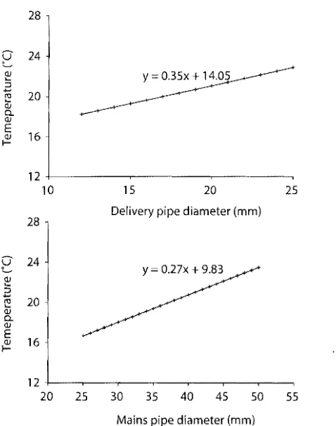
Figure 7.6. Effect ofdelivery (bottom) and main (top) pipe diameters on water temperature (P=O.OOOI).
Bore (18.6 0c) and river water (19.0 0c) is generally cooler than the main water (23.1 °C) supply (Figure 7.2). Using bore or river water can obviously assist producers to reduce water temperatures in piggery buildings and potentially capture the production benefits associated with optimal water temperatures.
Using water pipes that are buried below ground (18.5 0c) could be used effectively to keep drinking water colder (Figure 7.3) than water supplied via above ground pipes (22.0 °C). As a matter of fact approximately 3.5 °C temperature reduction can be achieved in water temperature by simply burying water pipes below ground. This 3.5 °C reduction is quite large and could potentially encourage pigs to increase their water intake. Increased water intake would be expected to lead to increased feed intake, resulting in growth rate and efficiency improvements (Bigelow and Houpt, 1988; Yang et al., 1984).
Low-pressure systems had lower drinking water temperatures (19.7 °C) than high water pressure (20.8 0c) systems (Figure 7.4). It is difficult to explain why low pressure systems result in reduced water temperatures. This effect is independent of the effect ofthe main supply running at higher pressure and so the explanation for this could lie in the natural physical relationship between
7. Water temperature on farms and the effect of warm drinking water on pig growth
temperature and pressure. High-pressure systems are usually associated with main water supplies and drinking systems being fed from main water supplies tend to have higher water temperatures. According to the results (Figure 7.5), drinking water systems that had in-shed reservoirs over 25 litres recorded significantly higher water temperature (24.5 DC) than drinking water systems that had smaller reservoirs (18.4 0C) or no reservoir (17.9 0C). However, this may be due to the quality of water storage facilities (i.e. uninsulated and in bad repair) rather than the existence and/or the size of water reservoirs. It is expected that poorly designed and maintained water reservoirs would increase drinking water temperature.
Drinking water temperature was positively correlated with the diameter of both the.mains and smaller delivery pipes. 'The positive effect of pipe diameter on drinking water temperatures might be a combination of many factors. However, the most likely explanation is that the larger pipes do absorb heat faster than smaller pipes, due to the larger surface exposed to hot air or direct sunlight. In addition, the speed of water flow is higher in smaller pipes; hence the water has less opportunity to absorb heat. Further studies are needed to better understand this effect.
In summary, the main effects on drinking water temperature in piggery buildings were season, source ofwater, position of piping, water pressure, size of in-shed water reservoir and diameter of main pipe and delivery pipes. In summer water temperature was significantly higher than at other times of the year and this highlighted the need for the producers to be aware of the increased risk of sub-optimal water temperature occurring during summer. Drinking water sourced from the main supply was warmer than drinking water sourced from bore or river water. Obviously manipulating or changing the source of drinking water is very difficult, if not impossible, but producers need to be aware of the potential effects of the water source on the likely temperature of drinking water supplied to pigs. Water supplied in high pressure pipes and supplied in pipes that were above ground had significantly higher temperature than drinking water supplied with low pressure system and from pipes that were buried underground, respectively. Itis not obvious why low pressure systems result in reduced water temperatures, but is possible that the physics of the positive relationship between pressure and temperature at constant volume is the cause. Watering systems that had water reservoirs larger than 25 Htres recorded higher drinking water temperatures. 'This may be due to the quality of water storage facilities (i.e. uninsulated and in bad repair) rather than the existence and/or the size of water reservoirs, as poorly designed and maintained water reservoirs obViously tend to increase drinking water temperatures. Thus producers do need to ensure that in-shed water reservoirs are maintained regularly and kept in good working order, including adequate insulation. Drinking water temperature was positively correlated with the diameter of both the main and smaller delivery pipes. The most likely explanation is that the larger pipes do absorb heat faster than smaller pipes, due to the larger surface exposed to hot air or direct sunlight. In addition, the speed of water flow is higher in smaller pipes; hence the water has less opportunity to absorb heat. However, manipulation of all these factors will require careful consideration.
No preViously published articles have been found by the authors of this chapter that would identify the statistically significant factors influencing drinking water temperatures in piggery
T. Banhazi and D. Rutley
bUildings. Thus this study results would have significant impact on current knowledge related to the appropriate management of drinking systems on farms.
I
'I
,I
,!
7.3.2 Study component 2 -on-farm experiment: effect ofwater temperature on pig
growth rate
The experimental component of the study was conducted at the University of Adelaide, Roseworthy campus research piggery. A preliminary study before the actual experiment confirmed that the aquarium heaters (Fluval Aquarium Heater, Hagen Inc. Montreal, Canada) selected for water temperature control were simple to install, cost effective and easy to maintain. The heaters were capable of achieving good control of water temperature within a very narrow temperature range (28.5±0.4 °C), which was quite independent of surrounding air temperatures (21.5±0. 9°C), There was a close association between the temperature of water in the overhead tank (28.6±0.4 °C) and that supplied to the pigs under experimental conditions (28. 16±0.45 0c). The results of this preliminary equipment trial demonstrated that the water temperature in the tanks and supplied to the animals was well controlled.
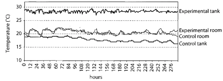
Figure 7.7 shows the water and air temperatures in the experimental and control rooms over a 12 day period, as an example. The average air temperature for the treatment group was 21.8±0.7 °C and 21.4±0.8 °C for the control group for the duration of the trial. Pigs in the treatment group received water heated to 28.4±0.4 °C, while the control group received unheated water at an average temperature of 17.8±0.9
0c.
The growth rates of experimental and control pigs are shown in Figure 7.8. Growth rate was suppressed (P<0.05) by 58 grams/day in the group receiving the heated water. This was a reduction of 17% of the daily growth rate.
This experiment demonstrated the significantly adverse effect of warm drinking water. Based on the assumption that this lost growth would be equivalent for weaner pigs in this shed throughout the year) the loss of 58 grams per day would equate to a loss of 15.9 kg. At $3.00 per kg carcass
30
G 2S
3 ~ "-
room 20
~
QJ
0
E lS
QJ
f
lO
~~Experimental tank
,
Control room
Control tank
o~~~~~~~~~~~~~~g~~~~~~~~
- t - , . - , . - , . - , . - - - N N N N N N N
[image:10.534.87.460.467.603.2]hours
Figure 7.7. Water and air temperatures in the control and experimental rooms.
7. Water temperature on farms and the effect of warm drinking water on pig growth
o 450 , ---,
>:.
'"
:!2
.EJ 400
c: 'ro
O'l
.?:
'ro
...1-,...
'0 350
<iJ O'l
t T
'"
OJ I)~ 300 I .
I I
---J [image:11.553.164.396.80.210.2]Cool water Heated water
Figure 7.B. Average daily gain for the weaner pigs supplied with heated and unheated water (mean ± Sf).
weight with a 75% dressing per cent this would cost from $45 to $50 per weaner capacity in the shed. If we acknowledge that the average summer temperature of drinking water in QLD was 25°C, the 7 °C increase in water temperature for Y4 of the year, assuming a linear response as temperature increases, would equate to a loss of $8 per weaner space in the shed, $8,000 per shed per year for a 1000 head weaner shed.
Although losses under commercial conditions may not be as large as calculated above, producers should be aware of the potentially harmful effects of sub-optimal drinking water temperatures. It is important to note that during this study a very stable and relatively warm drinking water temperature was achieved. In commercial conditions there is usually larger daily temperature variation, allowing pigs to modify drinking behaviour and consume water during the cool parts of the day, mitigating the relatively large difference in growth rate found in this experiment. However, it is also important to note that this growth rate reduction was demonstrated with optimal ambient air temperature in conjunction with warm drinking water.
Limited amount of previously published papers were identified in the literature that would discuss the effects of water temperatures on growth rates in pigs. However, the few articles that were identified essentially supported the results ofthis current study (Brew et al., 2011; Jeon et al., 2006;
Kruse et al.! 2011). For example, a study conducted on the water intake of sows demonstrated a
negative relationship between water intake and relative body weight loss of sows expressed as a percentage of original body weight (Kruse et al., 2011). Another study demonstrated that sows drinking either 10°C or 15 °C water had significantly highe~ water and feed intake rates than sows drinking water at the temperature of 22°C resulting in higher estimated milk production rates (Jeon et al., 2006). These studies therefore indirectly confirmed the results of the current study
indicating a link between (1) increased water intakes and production rates as well as linking (2) drinking water temperatures and water consumption rates. Water has been regarded by many as a 'neglected nutrient' in pig production and the management of drinking water is obviously an
important aspect of good farm management practices (Brooks and Carpenter, 1990). 'Ihis chapter II:
suggested ways ofreducing the impact ofsub-optimal drinking water temperatures on pig growth
:~
r
r""'i'
II
I"
ill
ill
I::1'1
.,
:11:
"1'
1/1
I
rL.
T. Banhazi and D. Rutley
by implementing a few simple construction and management principles in relation to watering systems installed on pig farms.
7.4 Conclusions
As a result of this research the understanding of factors affecting drinking water temperature in piggery buildings has improved. In addition, the likely effect of warm drinking water temperature on growth was quantified.
Factors identified to be affecting drinking water temperature in piggery buildings included season, source of water, position of piping, water pressure, size of in-shed water reservoir and diameter of main and delivery pipes. Careful management of these factors could aid the provision of optimal drinking water temperature and enhance growth throughout the year.
Under experimental conditions approximately 10 °C water temperature increase resulted in 58 g/day growth rate reduction. Although it was recognised that under commercial conditions the production efficiency loss might not be that significant, producers should be aware of the importance and magnitude of the losses from not providing drinking water to pigs within the optimal temperature range.
Acknowledgements
We wish to acknowledge the financial support of the Pig Research and Development Corporation (PRDC) and the important contribution of producers (including the project partner, CEFN Pty. Ltd.), their managers and staff who kindly donated their time and facilities. We would also like to thank Dr C. Cargill (South Australian Research and Development Institute, SARDI), who was instrumental in obtaining funding for the project; Prof John Black,
0.
Black Consulting) and Prof J. Hartung (Hannover University, Germany) for their professional advice. The important contribution of Mr J. Weigel of SARDI involved in the study is also gratefully acknowledged.References
Banhazi, T.M., Seedorf,
J.,
Rutley, D.L. and Pitchford, WS., 2008. Identification 'of risk factors for sub optimal housing conditions in Australian piggeries - Part II: airborne pollutants. Journal of AgriculturalSafety and Health 14: 21-39.
Bigelow, J.A. and Houpt, T.R., 1988. Feeding and drinking patterns in young pigs. Physiology & Behavior 43: 99-109.
Black, J.L., Giles, L.R., Wynn, P.C, Knowles, A.G., Kerr, CA., Jone, M.R., Gallagher, N.L. and Eamens, G.J., 2001. A review factors limiting the performance of growing pigs in commercial environments. In: Cranwell, ED. (ed.) Manipulating pig production VIII. Australasian Pig Science Association, Victorian
Institute of Animal Science, Werribee, Victoria, Australia, pp. 9-36.
Brew, M.N., Myer, R.n, Hersom, M.J., Carter, J.N., Elzo, M.A., Hansen, G.R. and Riley, D.G., 2011. Water intake and factors affecting water intake of growing beef cattle. Livestock Science 140: 297-300.
158 Livestock housing
7. Water temperature on farms and the effect of warm drinking water on pig growth
tng Brooks, P.H. and Carpenter, J.L., 1990. The water requirement of growing-finishing pigs: Theoretical and practical considerations. In: Haresign, W. and Cole, D.J.A. (eds.) Recent advances in animal nutrition. Butterworths, Boston, MA, USA, pp. 115-136.
Chen, Y.-H. and Chen, H., 1999. Incomplete covariates data in generalized linear models. Journal of Statistical Planning and Inference 79: 247-258.
, in Demidenko, E. and Stukel, T.A., 2002. Efficient estimation of general linear mixed effects models. Journal
lre of Statistical Planning and Inference 104: 197-219.
Jeon, J.H., Yeon, S.c., Choi, Y.H., Min,
w.,
Kim, S., Kim, P.'. and Chang, H.H., 2006. Effects of chilled drinking water on the performance oflactating sows and their litters during high ambient temperatures~ed under furm conditions. Livestock Science 105: 86-93.
j
nd Jones, R. and Nicol, c.J., 1998. A note on the effect of <;ontrol of the thermal environment on the well-being
01;1 of growing pigs. Applied Animal Behaviour Science 60: 1-9.
Kruse, S., Traulsen, I. and Krieter,
J.,
2011. Analysis of water, feed intake and performance oflactating sows. Livestock Science 135: 177-183.in Le Dividich, J. and Herpin, P., 1994. Effects of climatic conditions on the performance, metabolism and
,ns health status of weaned piglets: a review. Livestock Production Science 38: 79-90.
he Morrison, R.S., Smith, c.A. and Argent, C.D., 2007. The effect of cooled drinking water on the lactation he performance of gilts and parity 1 sows. In: Paterson, J.E. and Baker, J.A. (eds.) Manipulating pig
production XI. APSA, Werribee, VIC, Australia, pp. 37.
Pointon, A.M., Cargill, c.P. and Slade, }., 1995. TIle good health manual for pigs. Pig Research and Development Corporation, Canberra, Australia.
SAS, 1989. SAS/STAT" User's Guide, Version 6, Fourth Edition, Volume 2. SAS Institute, Cary, NC, USA. :m StatSoft, I., 2001. STATISTICA. StatSoft, Inc., Tulsa, OK, USA.
ty.
Van der Peet-Schwering, C.M.C., Vermeer, H.M. and Beurskens-Voermans, M.P., 1997. Voluntary andke
restricted water intake of pregnant sows. In: Bottcher, R.W. and Hoff, S.J. (eds.) 5th Internationalks
Symposium - Livestock Environment V, 29-31 May 1997, Bloomington, MN, USA. American Societyld
of Agricultural Engineers, pp. 959-964.Yang, T.S., Price, M.A. and Aherne, EX., 1984. The effect of level of feeding on water turnover in growing pigs. Applied Animal Behaviour Science 12: 103-109.
Zhang, Y., Barber, E.M. and Sokhansanj, S., 1992. A model of the dynamiC thermal environment in livestock buildings. Journal of Agricultural Engineering Research 53: 103-122.
l
I I