LiDAR data for DEM generation and flood plain mapping

University  of  Southern  Queensland  

Faculty  of  Health,  Engineering  and  Sciences  

LiDAR  Data  for  DEM  Generation  

and  Flood  Plain  Mapping

A  dissertation  submitted  by  

Maxwell  James  Burke  

In  fulfilment  of  the  requirements  of  

Courses  ENG4111  and  ENG4112  Research  Project  

Towards  the  degree  of  

Bachelor  of  Spatial  Science  (Surveying)  

Submitted:  October,  2013  

Abstract  

High-­‐resolution  Digital  Elevation  Model  (DEM)  is  a  key  spatial  dataset  for  flood  plain   mapping   and   catchment   management.   On   the   10th   _{of   January   2011,   heavy   rainfall}   caused  flash  flooding  through  Toowoomba  city  and  central  business  district  resulting  in   loss  of  life  and  significant  damage  to  public  and  private  property.  Effective  flash  flood   forecasting   is   a   big   challenge   that   requires   accurate   catchment   spatial   information.   Much   research   has   been   undertaken   on   the   use   of   airborne   LiDAR   data   to   generate   high-­‐resolution  DEM.  

The  aim  of  this  report  is  to  determine  the  suitability  of  using  airborne  LiDAR  data  for   flood  plain  mapping  and  catchment  management.  Airborne  LiDAR  data  will  be  used  to   generate  a  high  resolution  DEM  for  a  section  of  West  Creek,  part  of  the  Gowrie  Creek   catchment,   Toowoomba,   Queensland.   Accuracy   of   this   high-­‐resolution   DEM   was   verified  using  GPS  survey  equipment  to  gather  point  data  over  the  study  area.  Flood   zone,  inundation  depth  and  water  volume  was  extracted  from  the  LiDAR  derived  DEM   for   flood   surface   levels   indicative   of   the   2011   floods.   These   datasets   were   verified   using  the  GPD  derived  DEM.    

Disclaimer  

University  of  Southern  Queensland  

Faculty  of  Health,  Engineering  and  Sciences  

ENG4111  and  ENG4112  Research  Project  

Limitations  of  Use  

The   council   of   the   University   of   Southern   Queensland,   its   Faculty   of   Health,   Engineering  and  Sciences,  and  the  staff  of  the  University  of  Southern  Queensland,  do   not   accept   and   responsibility   for   the   truth,   accuracy   or   completeness   of   material   contained  within  or  associated  with  this  dissertation.  

Persons  using  all  or  any  part  of  this  material  do  so  at  their  own  risk,  and  not  at  the  risk   of   the   Council   of   the   University   of   Southern   Queensland,   its   Faculty   of   Health,   Engineering  and  Sciences  or  the  staff  of  the  University  of  Southern  Queensland.  

This   dissertation   reports   and   educational   exercise   and   has   no   purpose   or   validity   beyond  this  exercise.  The  sole  purpose  of  the  course  pair  entitled  “Research  Project”  is   to   contribute   to   the   overall   education   within   the   student’s   chosen   degree   program.   This  document,  the  associated  hardware,  software,  drawings,  and  other  material  set   out  in  the  associated  appendices  should  not  be  used  for  any  other  purpose:  if  they  are   so  used,  it  is  entirely  at  the  risk  of  the  user.  

Dean  

Faculty  of  Health,  Engineering  and  Sciences  

Certification  

I   certify   that   the   ideas,   designs   and   experimental   work,   results,   analysis   and   conclusions  set  out  in  this  dissertation  are  entirely  of  my  own  efforts,  except  where   otherwise  indicated  and  acknowledged.  

I   further   certify   that   the   work   is   original   and   has   not   been   previously   submitted   for   assessment  in  any  other  course  or  institution,  except  where  specifically  stated.  

Maxwell  James  Burke  

Student  number:  U1002661  

Acknowledgements  

I   would   like   to   acknowledge   that   this   research   was   carried   out   under   the   principal   supervision  of  Dr  Xiaoye  Liu.  Dr  Liu  support  and  expertise  in  this  area  of  research  has   been  invaluable.  

Table  of  Contents  

Abstract  ...  2  

Disclaimer  ...  3  

Certification  ...  4  

Acknowledgements  ...  5  

List  of  Tables  ...  8  

List  of  figures  ...  9  

Chapter  1  –  Introduction  ...  11  

1.1   Introduction  ...  11  

1.2   Aim  of  this  Research  ...  12  

1.3   Expected  Benefits  ...  12  

1.4   Dissertation  Overview  ...  13  

Chapter  2  –  Literature  Review  ...  14  

2.1   Introduction  ...  14  

2.2   Flood  plain  mapping  ...  14  

2.3   LiDAR  technology  ...  15  

2.4   DEM  generation  and  accuracy  ...  16  

2.5   Conclusion  ...  18  

Chapter  3  –  Methodology  ...  19  

3.1   Introduction  ...  19  

3.2   Study  Area  ...  19  

3.3   Data  Acquisition  ...  20  

3.4   DEM  Generation  ...  23  

3.5   Validation  of  GPS  Data  Acquisition  ...  24  

3.8   Flood  Inundation  Depth  and  Volume  ...  30  

3.9   Conclusion  ...  31  

Chapter  4  –  Results  and  Discussion  ...  32  

4.1   Introduction  ...  32  

4.2   Validation  of  GPS  Data  Acquisition  ...  32  

4.3   Elevation  Accuracy  of  Airborne  LiDAR  Derived  DEM  ...  36  

4.4   Flood  Zone  Delineation  ...  42  

4.5   Flood  Inundation  Depth  and  Volume  ...  47  

4.6   Conclusion  ...  49  

Chapter  5  –  Conclusions  ...  51  

5.1   Introduction  ...  51  

5.2   Further  Research  and  Recommendations  ...  51  

5.3   Conclusion  ...  52  

Appendices  ...  53  

Appendix  A  -­‐  Project  Specification  ...  53  

Appendix  B  –  Risk  Assessment  Matrix  ...  55  

Appendix  C  –  LiDAR  Report  for:  Toowoomba  Regional  Council  2010  LiDAR  Capture   Project.  ... 66  

Appendix  D  –  Project  Timeline  ...74  

List  of  Tables  

Table  1  LiDAR  meta-­‐data  (Schlencker  Mapping  Pty  Ltd,  2010,  p4)  ...  22  

Table  2  Land  cover  classes  used  in  vertical  accuracy  analysis  with  descriptions  ...  27  

Table  3  Stream  water  levels  (metres),  Canley  stream  gauge,  Gowrie  Creek  (QLD  DNRM,   2012).  ...  30  

Table  4  Elevation  errors  in  validation  surveys  in  metres.  ...  34  

Table  5  Elevation  errors  in  validation  survey  in  metres,  with  and  without  retaining  wall.  ...  35  

Table  6  Elevation  error  (m)  of  LiDAR  generated  DEM.  ...  38  

Table  7  Elevation  error  (m)  of  LiDAR  generated  DEM  across  grade  classes.  ...  39  

Table  8  Elevation  error  (m)  of  LiDAR  generated  DEM  across  land  cover  classes.  ...  41  

Table   9   Flood   zone   surface   areas   for   each   flood   water   level   surface   across   GPS   generated  DEM  and  LiDAR  generated  DEM  ...  45  

Table  10  Flood  inundation  depth  and  volume  for  each  flood  water  surface  across  GPS   generated  DEM  and  LiDAR  generated  DEM.  ...  49  

List  of  figures  

Figure  18  Raster  images  of  flood  inundation  depths  for  4.5m  water  level.  GPS  is  shown   on  left  and  LiDAR  on  right.  ...  48   Figure  19  Raster  images  of  flood  depths  for  3.5  metre  water  level.  GPS  is  shown  on  left   and  LiDAR  on  right.  ...  48  

Chapter  1  –  Introduction  

1.1Introduction  

Around   lunch   time   on   Monday   the   10th   _{of   January   2011,   without   warning,   intense}   rainfall   over   the   Gowrie   Creek   Catchment   caused   severe   flash   flooding   through   the   Toowoomba  CBD  (Central  Business  District)  resulting  in  loss  of  life  and  great  damage  to   property.  Heavy  rainfall  lasted  not  much  longer  than  an  hour  and  flood  waters  peaked   only   1.5   to   2   hours   after   the   rainfall   began   giving   little   warning   time.   Accurate   flash   flood   forecasting   for   specific   locations   is   challenging   but   necessary   for   the   design   of   flood  mitigation  measures  to  avoid  repeats  of  the  damage  explained  above.    

Figure  1  Flooded  Toowoomba  CBD  [Source:  Sydney  Morning  Herald]  

airborne  LiDAR  data  to  provide  accurate  data  across  large  areas  of  catchments  that  can   be  useful  for  accurate  flash  flood  prediction.  

1.2Aim  of  this  Research  

The  aim  of  this  research  is  to  determine  the  suitability  of  airborne  LiDAR  data  for  high-­‐ resolution   DEM   generation   and   flood   plain   mapping.   LiDAR   output   will   be   verified   using  GPS.  This  aim  is  broken  into  the  following  research  objectives:  

a) Use  airborne  LiDAR  point  data  to  generate  a  high  resolution  DEM  over   specified  study  area.  

b) Verify  accuracy  of  LiDAR  generated  DEM  by  GPS  data  acquisition.  

c) Use   LiDAR   generated   high-­‐resolution   DEM   to   delineate   flood   zone   for   typical  flash  flood  water  levels.  

d) Verify  accuracy  of  flood  zone  delineation  by  GPS.  

e) Use   LiDAR   generated   high-­‐resolution   DEM   for   flood   inundation   depth   and  water  volume  calculations.  

f) Verify  flood  inundation  depth  and  water  volume  by  GPS.  

1.3Expected  Benefits  

1.4Dissertation  Overview  

This   dissertation   contains   five   main   chapters.   These   chapters   are   given   a   brief   description  below:  

Chapter  1  Introduction  –  Gives  an  introduction  to  the  topic  of  research.  The  aims  of   the  research  are  provided.  Background  information  regarding  the  topic  is  discussed  as   well  as  perceived  benefits  of  the  research.  

Chapter  2  Literature  Review  –  Provides  a  summary  of  the  literature  review  undertaken   for   this   dissertation.   It   is   broken   into   three   topic   areas;   flood   plain   mapping,   LiDAR   technology  and  DEM  generation  and  accuracy.  

Chapter  3  Methodology  –  This  chapter  discusses  the  methods  used  to  fulfil  the  aims  of   the   research.   Discussion   is   included   regarding   the   study   area,   data   acquisition,   DEM   generation   and   analysis,   flood   zone   delineation   and   flood   inundation   depth   and   volume  analysis.  

Chapter  4  Results  and  Discussion  –  Provides  output  data  from  the  methodology  and   discussion  of  prevalent  trends  and  relationships  between  airborne  LiDAR  accuracy  and   high-­‐resolution  DEM  applications  in  flood  plain  mapping.  

Chapter  5  –  Provides  a  conclusion  to  the  dissertation  

Chapter  2  –  Literature  Review  

2.1Introduction  

A   literature   review   was   undertaken   in   regard   to   three   key   areas   consisting   of,   flood   plain  mapping,  LiDAR  technology  and  DEM  generation  and  accuracy.  This  chapter  aims   to   give   insight   into   previous   research   and   findings   in   this   area   as   well   as   explaining   some  key  concepts  of  this  area  of  study.  

2.2Flood  plain  mapping  

Flood   plain   mapping   involves   the   formation   of   a   number   of   models   for   analysis   and   management  such  as  topographic  surface  models,  two-­‐dimensional  hydraulic  surface   flow   models   and   thematic   land   cover   maps   (Hollaus,   et   al.,   2005).   The   DEM   and   its   derived  parameters  such  as  slope,  aspect  and  drainage  network  forms  the  base  input   data   for   these   models   and   therefore   the   accuracy   of   the   input   DEM   will   have   direct   influences   on   the   output   models.   Increased   accuracy   of   the   input   DEM   is   crucial   in   minimizing  the  uncertainties  of  flood  modeling  and  simulation  results  (Hollaus,  et  al.,   2005).  

McDougall,  et  al.  (2008)  reports  on  the  accuracy  requirements  of  DEMs  for  catchment   management.   Coverage   and   accuracy   requirements   for   different   applications   of   catchment   management   were   determined   in   2007   by   a   workshop   of   18   participants   representing   key   stakeholders,   for   Queensland.   The   coverage   and   accuracy   requirements   for   the   application   of   “Disaster   planning   and   management   (flood   and   fire)”  is  defined  as  +/-­‐1m.  However,  other  applications  that  may  be  applicable  to  flash   flood   prediction   have   coverage   accuracy   requirements   of   <0.5m   including,   “Hydrological   modelling”,   “Insurance   risk   and   assessment”   and   “Land   and   water   management  plans”  (McDougall,  et  al.,  2008).    

depth  are  usually  calculated  for  a  flood  event  with  a  specific  return  period  (de  Moel  et   al.,  2009).  Moel  and  Aerts  (2010)  conducted  research  into  the  effects  of  uncertainty  in   land  use,  damage  models  and  inundation  depth  on  flood  damage  estimates.  Results  of   the  research  indicate  that  when  an  uncertainty  of  250  cm  is  assumed  for  inundation   depth,   a   total   uncertainty   surrounding   the   final   damage   estimate   in   the   case   study   area  can  vary  up  to  a  factor  5-­‐6.  In  other  words,  the  lowest  estimate  for  flood  damage   is   5-­‐6   times   lower   than   the   highest   estimate   of   damage   (Moel   and   Aerts,   2010).   Accuracy  of  inundation  depth  is  clearly  critical  in  estimating  flood  damage.  

2.3LiDAR  technology    

LiDAR,  also  referred  to  as  airborne  laser  scanning,  light  detection  and  ranging,  or  laser   altimetry,   is   an   active   remote   sensing   technique,   which   was   originally   designed   to   measure   the   topography   of   the   Earth’s   surface   (Hollaus,   et   al.,   2005).   A   laser   emits   short   infrared   pulses   towards   the   Earth’s   surface   and   a   photodiode   measures   the   backscattered  echoes  (Hollaus,  et  al.,  2005).  LiDAR  technology  has  been  studied  for  a   considerable  time  period  since  as  early  as  the  1960’s  and  continues  to  be  an  area  of   active  research  and  development  (Flood,  2001).  Though  airborne  LiDAR  data  has  been   commercially   in   use   since   the   mid   1990’s   it   is   still   developing   rapidly   in   regards   to   sensor  technology  and  data  processing.  Developments  in  LiDAR  technology  allow  high-­‐ density  point  data  to  be  captured  for  more  affordable  prices.  High-­‐density  point  data   allows   terrain   to   be   represented   in   much   detail   (Liu,   2008).   As   a   result   of   these   developments  LiDAR  data  has  become  a  major  source  of  digital  terrain  information  for   a  variety  of  applications  including  hydraulic  modelling  and  flood  plain  mapping  (Raber,   et  al.,  2007).  

Elevation   error   of   LiDAR   was   shown   to   be   the   function   of   a   number   of   variables   including   LiDAR   system   measurements,   horizontal   displacement,   interpolation   error   and   surveyor   error.   Analysis   of   elevation   error   was   undertaken   across   a   number   of   land  cover  and  grade  classes.  The  results  of  the  study  show  that  elevation  root  mean   square   errors   for   LiDAR   data   were   17   to   26   cm.   The   highest   errors   were   shown   to   occur   over   steep   land   as   the   horizontal   error   in   this   land   type   introduced   further   elevation   error.   LiDAR   measurement   over   land   of   steep   slopes   with   grades   approximately   25   degrees   were   shown   to   contain   elevation   errors   twice   as   large   as   data  collected  over  slopes  of  1.5  degrees.  Errors  over  flat  surfaces,  even  forested  ones,   were  shown  to  be  very  low  compared  to  other  sources  of  digital  elevation  data  such  as   photogrammetry  (Hodgson  and  Bresnahan,  2004).  

There  have  been  a  number  of  other  studies  that  assess  the  accuracy  of  LiDAR  derived   elevations  for  various  study  areas.  Adams  and  Chandler  (2002)  found  a  LiDAR  derived   elevation  accuracy  of  26  cm  and  found  improved  results  over  sloping  terrain  compared   to  DEMs  derived  from  digital  photogrammetry.  Bowen  and  Waltermine  (2002)  found   an  overall  elevation  accuracy  of  43  cm.  Cobby  et  al.  (2000)  found  an  LiDAR  elevation   accuracy  of  17  cm  for  data  gathered  over  grass  and  cereal  crop  land  cover.    

2.4DEM  generation  and  accuracy  

Liu   (2008)   provides   a   study   into   the   effective   processing   of   raw   LiDAR   data   and   the   generation   of   high   resolution   DEM.   Methods   regarding   DEM   generation,   LiDAR   data   reduction,   LiDAR   data   filters,   and   interpolation   are   discussed.   These   will   be   of   great   importance   to   the   aims   of   this   report   as   reducing   redundant   information   and   generating  an  accurate  DEM  efficiently  is  of  importance.  Liu  (2008)  concludes  that  the   filtering  of  ground  and  non-­‐ground  data  is  the  most  critical  step  in  generation  of  an   accurate  DEM  from  LiDAR  data.  Also  of  worth  is  the  extraction  and  inclusion  of  critical   elements,  such  as  breaklines,  in  maintaining  accuracy  without  excessive  redundancies   (Liu,  2008).  

use  studies,  they  introduce  significant  errors  into  a  DEM  if  not  filtered.  Dowman  and   Fischer  (2001)  conducted  research  into  the  elevation  errors  of  airborne  LiDAR  derived   DEM  using  multiple  returns.  These  authors  found  significant  errors  of  up  to  4m  RMSE   over  flat  ground  when  no  filtering  was  applied  (Downman  and  Fischer,  2001).  Zhang,  et   al.  (2003)  provides  a  study  on  a  progressive  morphological  filter  to  remove  non-­‐ground   points  from  airborne  LiDAR  data.  The  filter  is  developed  and  tested  on  mountainous   and  flat  urbanized  areas  with  apparent  success.  An  effective  and  accurate  method  of   removing   non-­‐ground   data   from   LiDAR   data   is   critical   in   generation   accurate   high   resolution  DEMs  (Zhang,  et  al.,  2003).    

Liu   and   Zhang   (2010)   provide   a   study   into   the   automated   delineation   of   drainage   networks  from  high  resolution  DEM.  As  the  drainage  network  is  one  of  main  factors  in   flood  prediction,  accurate  means  of  extracting  it  are  paramount.  Liu  and  Zhang  (2010)   assess  existing  methods  for  drainage  network  extraction  and  focus  on  extraction  using   the   Arc   Hydro   extension   of   ArcGIS   with   different   threshold   limits   (the   minimum   upstream  drainage  area).  The  study  concludes  with  the  evidence  that  high  resolution   DEMs  are  required  for  detailed  drainage  networks  as  they  can  provide  adequate  data   for  drainage  network  extraction  using  smaller  threshold  values.  

Assessing  the  accuracy  of  LiDAR  derived  DEM  is  a  key  outcome  of  this  research  project.   A  commonly  accepted  method  to  perform  an  empirical  assessment  of  LiDAR  generated   DEM  accuracy  is  to  use  the  root  mean  square  error  (RMSE)  statistic  based  on  survey   spot  levels  (Raber  et  al.,  2007).  The  RMSE  formula  is  as  follows:  

𝑅𝑀𝑆𝐸!"#$%  !"#$%&'()*+#=

Σ(𝑍!"#$%−𝑍!"#$%&)!

𝑛  

Where:  

ZLiDAR  =  Elevation  of  LiDAR  point  (m)  

ZSurvey  =  Elevation  of  surveyed  point  (m)  

The  RMSE  value  provides  a  tangible  and  realistic  estimate  of  errors  most  likely  to  be   encountered  for  LiDAR  observations.  This  will  be  used  in  analysing  the  elevation  errors   of  airborne  LiDAR  generated  high  resolution  DEM.  

2.5Conclusion  

This  chapter  has  discussed  key  concepts  of  the  study  area  as  well  as  reviewing  research   and  findings  of  relevant  literature.  Flood  plain  mapping  was  the  first  topic  researched.   Data  requirements  for  flood  plain  mapping  were  identified  and  the  importance  of  an   accurate   DEM   was   noted   as   many   output   models   are   based   of   this   key   data   set.   Accuracy   requirements   of   DEMs   for   flood   plain   mapping   were   defined   and   the   application   of   flood   plain   mapping   in   regards   to   damage   estimates   was   discussed.   Secondly,   LiDAR   technology   was   researched.   Background   information   on   this   technology  was  provided  including  history  of  use  and  expected  error  sources.  Thirdly,   DEM   generation   and   accuracy   was   researched.   Research   regarding   filtering   of   non-­‐ ground  points  and  accurate  DEM  generation  was  presented.  Use  of  DEM  for  flood  plain   modelling   was   discussed   as   well   as   statistical   methods   to   analyse   DEM   elevation   accuracy.  

Chapter  3  –  Methodology  

3.1Introduction  

This  chapter  will  present  the  different  stages  of  planning,  resources,  data  acquisition,   data  processing  and  analysis  in  order  to  meet  the  aims  of  the  research.  It  will  cover:  

• Study  Area  

• Data  Acquisition  

• DEM  Generation  

• Validation  of  GPS  Data  Acquisition  

• Elevation  Accuracy  of  Airborne  LiDAR  Derived  DEM  

• Flood  Zone  Delineation  

• Flood  Inundation  Depth  and  Volume  

3.2Study  Area  

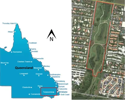
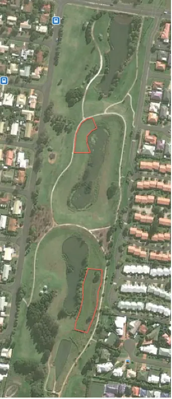
Figure  2  Study  area  –  Toowoomba,  Queensland  

Figure  2  shows  the  study  area  outlined  in  red.  It  extends  south  from  Stennar  Street,   bounded   by   Lemway   Avenue   to   the   west   and   Fay   Court   to   the   east,   until   past   the   fourth  detention  pond  as  shown.  

3.3Data  Acquisition  

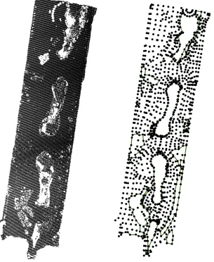
Two  types  of  data  were  required  for  this  research  project.  First,  LiDAR  point  data  was   obtained   to   generate   a   high-­‐resolution   DEM.   Second,   fieldwork   was   undertaken   to   collect  point  data  over  the  study  area  using  GPS  survey  equipment.  

Figure  3  displays  the  point  data  acquired  for  both  LiDAR  and  GPS  surveys  across  the   study  area.  

Figure  3  Data  points  across  study  area.  LiDAR  points  are  shown  on  the  left  and  GPS  points  on  the  right   The  LiDAR  data  was  sourced  from  a  Toowoomba  wide  LiDAR  survey  conducted  in  2010   by   Schlencker   Mapping   Pty   Ltd   for   Toowoomba   City   Council.   The   survey   covered   an   area  of  more  than  2760  square  kilometres  across  the  Toowoomba  Local  Government   Area   (Schlencker   Mapping   Pty   Ltd,   2010).   Schlencker   Mapping   provided   the   data   to   Toowoomba   City   Council   in   separated   layers   of   ground   and   non-­‐ground   points.   The   method  used  to  separate  the  point  data  into  ground  and  non-­‐ground  is  unknown.  As   can  be  seen  in  the  above  images,  the  density  of  LiDAR  observations  is  very  high  –  one   of   the   characteristics   of   LiDAR   data.   The   average   point   separation   is   1m   (Schlencker   Mapping  Pty  Ltd,  2010).  The  data  for  this  research  was  cropped  from  the  two  adjoin   1km  square  tiles  to  cover  the  West  Creek  study  area.  

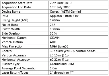
Table  1  shows  the  meta-­‐data  of  the  LiDAR  survey  was  provided  by  Schlencker  Mapping   (2010).    

Acquisition  Start  Date 29th  June  2010 Acquisition  End  Date 16th  July  3010

Device  Name Optech  ‘ALTM  Gemini’

IMU Applanix  ‘Litton  510’

Flying  Height  (AGL) 1200m

No.  of  Runs 242

Swath  Width 1000m

Side  Overlap 30  %

Horizontal  Datum GDA94

Vertical  Datum AHD

Map  Projection MGA  Zone56

Control 302  surveyed  GPS  control  points Vertical  Accuracy ±0.15m  @  1σ

Horizontal  Accuracy ±0.22m  @  1σ Surface  Type Ground  and  DTM Average  Point  Separation 1.0m

Laser  Return  Types 1st  _{through  to  4}th

Table  1  LiDAR  meta-­‐data  (Schlencker  Mapping  Pty  Ltd,  2010,  p4)  

Of  note  are  the  quoted  horizontal  and  vertical  accuracies  of  the  data.  The  results  were   validated   by   use   of   a   vehicle   mounted   GPS   rover   travelling   over   218   kilometres   of   roads  through  the  survey  area,  which  achieved  measurements  to  an  accuracy  of  +/-­‐.05   metres  (Schlencker  Mapping  Pty  Ltd,  2010).  It  is  worth  noting  that  this  validation  was   only  conducted  over  bitumen  and  gravel  roads  and  therefore  would  not  be  a  complete   validation  of  the  LiDAR  data  across  different  ground  covers.    

validation  of  LiDAR  accuracy  over  such  terrain.  It  must  be  noted  that  elevation  data  for   the  water  bodies  was  interpolated  and  not  collected.  It  was  considered  too  high  a  risk   to  enter  the  water  bodies  as  a  single  person  party  undertook  fieldwork  and  expensive   equipment  used  was  borrowed  from  the  University  of  Southern  Queensland.  In  total,   1460  data  points  were  collected  across  the  study  area.  

3.4DEM  Generation  

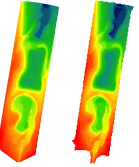
High   resolution   DEMs   were   generated   for   each   data   set   using   ESRI   ArcMap   10.1   software.  Figure  4  shows  the  two  DEMs.  

Figure  4  High  resolution  DEMs.  LiDAR  generated  DEM  is  shown  on  the  left  and  GPS  generated  DEM  is   shown  on  right.  

As  the  LiDAR  data  was  already  separated  into  ground  and  non-­‐ground  points,  the  DEM   was  generated  straight  from  the  ground  only  points.  

manipulation   of   triangles   to   ensure   correct   surface   modelling   along   banks,   retaining   walls  and  other  hard  breaklines.  A  high  resolution  DEM  was  then  generated  from  this   TIN  surface.  

3.5Validation  of  GPS  Data  Acquisition  

In   order   for   useful   comparison   and   analysis   of   LiDAR   generated   DEM,   the   GPS   generated   DEM   would   need   to   be   validated   as   an   accurate   representation   of   the   catchment  area.  Validation  of  the  GPS  survey  was  accomplished  by  re-­‐surveying  two   separate   areas   of   the   study   area   on   the   final   day   of   data   acquisition.   These   surveys   covered   an   area   of   approximately   4125m2,   and   consisted   of   101   points.   Similar   to   initial  GPS  processing,  TIN  surfaces  were  first  generated  across  each  validation  area  to   ensure  correct  three-­‐dimensional  surface  modelling.  DEMs  were  then  generated  from   these  TIN  surfaces.  

Figure  5  Site  map  showing  approximate  positions  of  GPS  validation  surveys  in  red.   3.6Elevation  Accuracy  of  Airborne  LiDAR  Derived  DEM  

The   central   objective   of   this   research   project   is   to   analyse   the   vertical   accuracy   of   airborne  LiDAR.  This  was  achieved  by  comparison  of  the  LiDAR  generated  DEM  and  the   GPS  generated  DEM  to  determine  the  difference  in  elevation  between  the  models.  This   was  undertaken  for  the  entire  data  set,  but  also  for  sub-­‐sets  of  the  data  to  determine   any   relationships   between   vertical   accuracy   and   grade   or   vertical   accuracy   and   land   cover.  

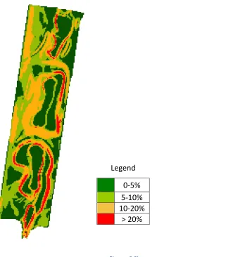
allow  appropriate  analysis  to  determine  the  influence  of  grade  on  vertical  error  in  the   LiDAR   generated   DEM.   To   achieve   this,   the   GPS   generated   DEM   was   copied   and   cropped  so  as  to  only  cover  the  grade  of  interest.  Elevation  comparison  between  the   cropped  GPS  generated  DEM  and  LiDAR  DEM  was  then  completed.  This  process  was   then  repeated  for  each  grade  class.  It  is  expected  that  as  grade  increases,  the  elevation   error  will  increase  (Hodgson  and  Bresnahan,  2004).  

Figure  6  Slope  map  

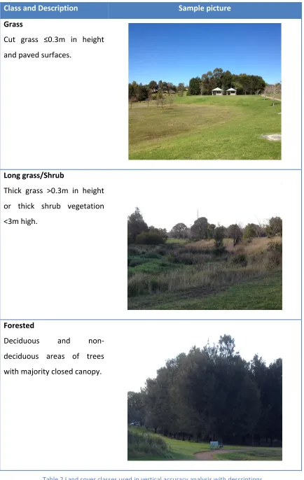
Analysis  of  vertical  error  in  the  LiDAR  generated  DEM  across  differing  land  cover  was   also  undertaken.  During  GPS  data  collection,  measurements  were  taken  to  delineate   areas  of  trees,  water  bodies,  cut  grass  (including  concrete  paths),  and  long  grass  and   shrubs.   For   purposes   of   analysis,   three   land   cover   classes   were   selected;   grass   (including   concrete   paths),   long   grass/shrubs,   and   trees.   Table   2   shows   typical   examples   of   these   areas   throughout   the   study   area   categorised   into   the   land   cover   classes  used  for  vertical  accuracy  analysis.    

Legend  

Class  and  Description   Sample  picture  

Grass  

Cut   grass   ≤0.3m   in   height   and  paved  surfaces.  

Long  grass/Shrub  

Thick   grass   >0.3m   in   height   or   thick   shrub   vegetation   <3m  high.  

Forested  

Deciduous   and   non-­‐ deciduous   areas   of   trees   with  majority  closed  canopy.  

Analysis  over  water  bodies  was  not  undertaken  due  to  the  absence  of  data  collection   through  water  bodies  as  stated  in  section  3.3.  Similar  to  analysis  over  different  grade   classes,  the  GPS  generated  DEM  was  copied  and  cropped  so  as  to  only  cover  the  land   cover   of   interest.   This   cropped   DEM   was   used   as   the   base   for   analysis   in   elevation   difference  of  LiDAR  generated  DEM  over  the  area.  This  method  was  repeated  for  each   land   cover   class.   It   is   expected   that   there   will   be   little   difference   between   vertical   errors  across  grass  and  tree  land  covers  (Hodgson  and  Bresnahan,  2004).  

In  order  to  provide  useable  data  on  the  expected  vertical  accuracies  of  LiDAR  data  the   root   mean   square   error   (RMSE)   for   elevation   values   will   be   calculated   for   the   entire   study  area  as  well  as  each  grade  and  land  cover  class.  This  statistical  analysis  is  useful   in   that   it   returns   values   in   the   units   of   the   variable   being   analysed.   In   this   way   the   elevation   RMSE   could   be   thought   of   as   the   expected   elevation   error   for   a   LiDAR   generated  DEM.  The  formula  used  for  RMSE  calculations  was  as  follows:  

𝑅𝑀𝑆𝐸_{!"#$%  !"#$%&'()*+#}= !(!!"#$%!!!"#)!

!           (1)  

Where:  

ZLiDAR  =  Elevation  of  LiDAR  generated  DEM  raster  cell  (m)  

ZGPS  =  Elevation  of  GPS  generated  DEM  raster  cell  (m)  

n  =  number  of  raster  cells  used  for  calculation  

3.7Flood  Zone  Delineation  

Basic  floodplain  mapping  applications  will  be  performed  on  each  DEM  surface  in  order   to  meet  the  other  key  objective  of  this  research.    

The  influence  of  DEM  errors  on  flood  zone  delineation  will  be  determined  by  creation   of  an  indicative  water  surface  level  for  a  flood  event  in  the  ESRI  ArcMap  10.1  software   package.  The  volumetric  difference  between  this  surface  and  the  GPS  generated  DEM   will  be  calculated  using  ArcMap  ‘Surface  Difference’  function.  A  polygon  feature  class  is   returned  where  each  polygon  is  classified  as  either  ‘above’,  ‘below’,  or  ‘equal’.  In  this   way  the  line  at  which  the  indicative  flood  water  surface  level  is  equal  to  the  ground   surface  is  defined  as  the  flood  zone  extent.  All  areas  where  the  water  surface  is  greater   than  the  ground  surface  would  be  classified  as  the  flood  zone.  The  same  calculations   will  be  repeated  for  the  LiDAR  generated  DEM.  Analysis  of  the  flood  zone  line  for  each   DEM  and  surface  area  of  the  flood  zone  will  be  undertaken  to  determine  how  flood   zone   location   and   area   across   the   surface   are   influenced   by   any   errors   in   the   LiDAR   generated  DEM.  

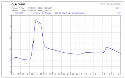
Table  3  Stream  water  levels  (metres),  Canley  stream  gauge,  Gowrie  Creek  (QLD  DNRM,  2012).   It  must  be  noted  that  the  surface  would  most  likely  be  an  inaccurate  representation  of   an   actual   flood   event   across   the   study.   However,   for   the   purpose   of   analysing   the   relationship  between  the  different  DEMs  and  the  same  water  level  surface,  the  actual   value   of   the   water   surface   is   in   some   ways   irrelevant,   as   it   remains   constant.   Delineation   of   actual   flood   zones   across   the   study   area   for   a   specified   flood   event   would  require  much  more  site-­‐specific  information  to  predict  a  water  surface  for  the   flood  event.  

3.8Flood  Inundation  Depth  and  Volume  

Analysis  of  the  influence  of  error  in  LiDAR  generated  DEM  on  flood  inundation  depth   and   volume   will   completed.   As   discussed   in   section   2.2   flood   inundation   depth   is   a   critical  data  set  for  flood  plain  mapping  in  the  application  of  flood  damage  estimation.   Relatively  low  uncertainties  between  0.1  -­‐0.25m  can  introduce  large  uncertainties  in   damage  estimates  (Moel  and  Aerts,  2010).  

calculations  will  be  undertaken  for  the  LiDAR  generated  DEM.  The  RMSE  value  will  be   calculated  in  order  to  analyse  the  expected  error  in  flood  inundation  depth  when  using   LiDAR  generated  DEM  for  flood  plain  mapping.  

3.9Conclusion  

This   chapter   discussed   what   methods   would   be   employed   to   fulfil   the   aims   of   this   research.   The   study   area   was   identified.   Data   acquisition   methods   were   discussed.   Generation  of  DEMs  and  analysis  methods  were  discussed.  The  methodology  discussed   above  provides  a  framework  for  the  presentation  of  results  and  discussion.  

Chapter  4  –  Results  and  Discussion  

4.1Introduction  

In   this   chapter   the   results   of   the   research   will   be   presented   and   discussed.   Output   from  ESRI  ArcMap  of  histograms  and  raster  images  will  be  presented  and  discussed  in   regards  to:  

• Elevation  accuracy  of  GPS  under  the  heading  Validation  of  GPS  

• Elevation  accuracy  of  Airborne  LiDAR  Derived  DEM  

• Flood  Zone  Delineation  

• Flood  Inundation  Depth  and  Volume  

4.2Validation  of  GPS  Data  Acquisition  

It   is   important   to   validate   the   original   GPS   survey   as   explained   in   section   3.5.   To   validate  the  elevation  of  the  original  GPS  survey,  the  elevations  of  the  DEMs  generated   from   the   validation   surveys   were   each   subtracted   from   the   elevations   of   the   DEM   generated  by  the  original  GPS  survey.  Figure  7  shows  the  resultant  raster  images  for   these   calculations   with   elevation   differences   in   metres   represented   by   the   different   colours.  

Figure  7  Raster  image  generated  by  GPS  generated  DEM  minus  validation  DEMs.  The  Northern   validation  survey  is  shown  on  the  left  and  the  Southern  validation  survey  on  the  right.  

the  validation  surveys  still  have  value  in  this  research.  Figure  8  and  Figure  9  show  the   ArcMap   output   of   the   elevation   differences   between   each   DEM   generated   by   the   validation  surveys  and  the  DEM  generated  by  the  original  survey.  ArcMap  was  used  to   generate   a   raster   image   of   the   squared   differences   of   the   elevations   across   corresponding   raster   cells.   These   values   were   used   to   calculate   RMSE   values   for   the   validation  surveys  as  seen  in  Table  4.  The  RMSE  values  are  high  at  0.089m  and  0.128m   for   the   North   and   Southern   surveys   respectively,   although   the   mean   differences   are   more   acceptable   at   -­‐0.037m   and   -­‐0.032m   for   the   Northern   and   Southern   surveys   respectively.  

Figure  9  ArcMap  10.1  output  of  elevation  difference  in  metres  between  Southern  validation  survey  and   original  GPS  survey.  

Survey   Mean   Standard  

deviation  

Raster  cell  count  

(n)  

Sum  square  

ΔV  

RMSE  

North   -­‐0.037   0.087   320   2.509   0.089   South   -­‐0.032   0.126   430   7.055   0.128  

Table  4  Elevation  errors  in  validation  surveys  in  metres.  

These  lines  are  calculated  as  having  continuous  elevations  of  constant  grade  between   the  nodes.  A  significant  vertical  error  is  therefore  generated  for  these  situations,  as  the   straight  line  of  constant  grade  will  ‘skip’  measured  points  from  another  data  set  along   the  curved  retaining  wall.    

To  demonstrate  this  added  error  source  along  curved  retaining  walls,  a  TIN  surface  for   the   Northern   validation   survey   was   generated   excluding   measured   points   along   the   curved   retaining   wall.   A   new   DEM   was   generated   from   this   cropped   surface   and   analysed   against   the   original   GPS   DEM   across   the   corresponding   area.   Table   5   demonstrates   an   improvement   of   this   cropped   area   in   terms   of   vertical   accuracy   by   removing  the  surface  over  the  curved  retaining  wall.    

Survey   Mean   Standard  

deviation  

Raster  cell  count   (n)  

Sum  square  

ΔV  

RMSE  

North   -­‐0.037   0.087   320   2.509   0.089   Crop  

North  

-­‐0.032   0.056   277   1.142   0.064  

Table  5  Elevation  errors  in  validation  survey  in  metres,  with  and  without  retaining  wall.  

Another  error  source  in  elevation  differences  between  the  GPS  surveys  is  the  inherent   vertical  errors  in  the  equipment  and  processes  used  for  data  collection.  The  GPS  was   used   in   a   rapid   real   time   kinetic   (RTK)   mode   taking   three-­‐second   observations   with   vertical   precisions   of   approximately   12-­‐35mm.   Difficulties   were   encountered   across   forested   areas   of   the   site   as   the   GPS   struggled   to   gain   high   vertical   precisions   and   would  regularly  lose  position  fix  when  in  these  areas.  Vertical  precision  through  these   areas  was  therefore  limited.  

could  be  argued  that  there  is  a  general  shift  as  the  mean  elevation  errors  are  both  very   close  to  -­‐0.035m,  however  for  the  purposes  of  flood  and  catchment  applications,  and   the  quoted  vertical  errors  of  +/-­‐0.15m  of  the  provided  LiDAR  data  as  seen  in  figure  3,   this  shift  would  be  negligible.  

In   regards   to   the   spread   of   vertical   differences   as   discussed   above,   it   would   be   recommended   for   future   studies   to   increase   point   spacing,   especially   across   curved   and   steep   changes   of   grades,   to   better   represent   the   surface   and   create   a   more   accurate  DEM.  The  elevation  errors  across  the  validation  surveys  do  present  the  need   for  higher  accuracy  point  acquisition  across  the  study  area.  This  could  be  achieved  by   longer  point  observation  times  or  combined  use  of  total  station  survey  equipment  for   forested  areas.  

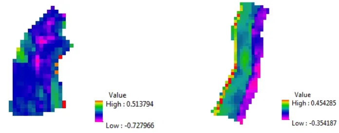
4.3Elevation  Accuracy  of  Airborne  LiDAR  Derived  DEM  

Figure  10  shows  the  resultant  raster  image  produced  by  subtracting  the  elevations  of   the   airborne   LiDAR   generated   DEM   from   the   elevations   of   the   GPS   generated   DEM.   The   colours   represent   the   calculated   elevation   difference   in   meters   as   shown.   This   visual  representation  shows  that  the  majority  of  the  study  are  (not  including  the  water   bodies)   returned   differences   in   height   between   +0.25m   and   -­‐0.25m   which   is   within   determined   accuracy   requirements   for   flood   plain   mapping   and   catchment   management  of  <0.5m  (McDougall,  et  al.,  2008).    

Figure  10  Raster  image  of  GPS  generated  DEM  minus  LiDAR  generated  DEM  

Figure  11  shows  the  output  statistics  for  the  above  raster  calculation.  ArcMap  software   was   used   to   calculate   the   square   elevation   difference   between   the   LiDAR   generated   DEM  and  the  GPS  DEM.  This  data  was  used  to  calculate  the  RMSE  value  of  the  LiDAR   elevations  according  to  equation  (1).  Table  6  provides  a  summary  of  these  statistics.   The  RMSE  for  LiDAR  elevation  across  the  entire  study  area  is  calculated  to  be  0.260m.   This  value  is  higher  than  the  quoted  vertical  accuracy  of  0.15m  in  Table  1,  although  this   is   not   surprising   as   the   means   of   validation   of   the   LiDAR   were   conducted   along   bitumen  and  gravel  roads  with  minimal  steep  grades  as  discussed  in  section  3.3.  We   can   see   that   the   mean   for   the   entire   dataset   is   -­‐0.159m   with   standard   deviation   of   0.226m,   which   confirms   the   deductions   from   the   raster   image   discussed   above.   The   mean  elevation  error  and  larger  histogram  area  to  the  left,  suggest  that  the  LiDAR  DEM   elevations  generally  above  the  GPS  generated  DEM  elevations  as  the  calculation  was   ordered   as   GPS   DEM   minus   LiDAR   DEM.   These   results   agree   with   other   empirical  

studies  that  have  been  conducted  to  date,  that  suggest  accuracies  of  26  cm  to  153  cm   RMSE   for   large-­‐scale   mapping   applications   (Adams   and   Chandler,   2002;   Bowen   and   Waltermine,  2002;  Hodgson  et  al.,  2003).  

Figure  11  ArcMap  10.1  output  of  elevation  differences  in  metres  between  entire  LiDAR  generated  DEM   and  GPS  generated  DEM  

  Mean   Standard  

Deviation  

Minimum   Maximum   RMSE  

Total  DEM   -­‐0.159   0.226   -­‐2.156   0.994   0.260  

Table  6  Elevation  error  (m)  of  LiDAR  generated  DEM.  

Figure  12  ArcMap  10.1  output  for  elevation  differences  in  metres  between  LiDAR  generated  DEM  and   GPS  generated  DEM  across  each  grade  class.  

  Mean   Standard  

Deviation  

Minimum   Maximum   RMSE  

Total  DEM   -­‐0.159   0.226   -­‐2.156   0.994   0.260   Grade  

Classes  

0-­‐5%   -­‐0.079   0.116   -­‐1.130   0.806   0.130   5-­‐10%   -­‐0.114   0.138   -­‐2.027   0.379   0.158   10-­‐20%   -­‐0.108   0.136   -­‐1.465   0.865   0.160   >  20%   -­‐0.169   0.277   -­‐2.235   0.709   0.309  

Table  7  Elevation  error  (m)  of  LiDAR  generated  DEM  across  grade  classes.  

The   results   from   elevation   comparison   of   DEMs   across   the   grade   classes   confirm   previous  research  that  one  of  the  sources  for  vertical  error  in  airborne  LiDAR  data  is   steep  grades  (Hodgson  and  Bresnahan,  2004).  This  relationship  is  apparent  in  Table  7  

0  –  5%   5  -­‐  10%  

were  we  see  increased  mean,  standard  deviation  and  range  of  errors  from  grade  class   0-­‐5%  to  grade  class  >20%.  There  is  little  difference  in  elevation  error  between  grades   classes   5-­‐10%   and   10-­‐20%,   however   the   elevation   errors   for   these   two   classes   are   larger  than  those  in  grade  class  0-­‐5%  and  smaller  than  those  in  grade  class  >20%.  So   while   the   relationship   of   increasing   grade   equalling   increasing   elevation   error   for   airborne   LiDAR   data   is   not   apparent   across   grades   5-­‐20%,   it   is   evident   for   grades   0-­‐   >20%.  

In  addition,  the  above  calculations  were  repeated  for  the  different  land  cover  classes.   Figure   13   shows   the   statistical   output   for   the   calculation   of   LiDAR   generated   DEM   minus  GPS  generated  DEM  for  each  land  class.  Table  8  summarises  these  results.  

Figure  13  ArcMap  10.1  output  for  elevation  differences  in  metres  between  LiDAR  generated  DEM  and  

GPS  generated  DEM  across  each  land  cover  class.    

Cut  grass   Long  grass/shrubs  

  Mean   Standard   Deviation  

Minimum   Maximum   RMSE  

Total  DEM   -­‐0.159   0.226   -­‐2.156   0.994   0.260  

Land  Cover            

Cut  grass   -­‐0.080   0.096   -­‐1.190   0.421   0.113   Long  

grass/shrubs   -­‐0.161   0.238   -­‐1.860   0.961   0.273   Forested   -­‐0.116   0.143   -­‐0.904   0.796   0.178  

Table  8  Elevation  error  (m)  of  LiDAR  generated  DEM  across  land  cover  classes.  

These  results  show  that  airborne  LiDAR  data  will  return  elevation  data  of  best  accuracy   across   areas   of   cut   grass   and   pavement   with   an   RMSE   of   0.113m,   under   half   of   the   RMSE  for  the  entire  study  area.  The  elevation  RMSE  was  also  low  across  forested  land   covers   at   0.178m   in   comparison   to   elevation   errors   of   the   entire   site.   These   results   confirm  by  past  research  that  shows  errors  over  flat  surfaces,  even  forested  ones,  are   very  low  compared  to  other  sources  of  digital  elevation  data  such  as  photogrammetry   (Hodgson   and   Bresnahan,   2004).   These   results   reflect   the   characteristics   of   forested   areas  of  the  site.  Forested  areas  consisted  of  tall  trees  with  closed  to  majority-­‐closed   canopies  with  little  to  no  other  ground  cover  in  the  form  of  long  grass  or  shrubs.  This   allows  any  LiDAR  signals  that  penetrate  the  canopy  acquire  a  bare  earth  elevation  with   ease.   Across   forested   areas   the   difference   between   ground   and   no-­‐ground   points   would   be   large   as   most   trees   were   in   a   height   range   of   5-­‐15m.   This   situation   would   allow  for  accurate  filtering  of  non-­‐ground  points  from  the  data  set  when  compared  to   land  covers  of  dense  undergrowth  close  to  the  bare  earth  surface.  These  land  cover   types   best   represent   the   vertical   accuracy   of   the   provided   airborne   LiDAR   data   as   quoted  in  Table  1.    

the  entire  study  area  elevation  RMSE  of  0.260m.  These  larger  elevation  errors  would   be  expected,  as  penetration  of  such  homogenous  thick  land  cover  by  airborne  LiDAR   scanners  would  be  difficult.  Separation  of  ground  and  non  ground  points  would  prove   to   be   a   further   source   of   error   over   these   land   covers   as   the   elevation   difference   between  the  bare  earth  and  the  top  of  the  grass  or  shrub  would  not  be  as  extreme  as   those   differences   in   forested   areas.   These   inaccuracies   have   been   evident   in   other   studies  that  returned  greatest  elevation  errors  over  homogenous  meadows  with  high   grass  and  shrubs  (Hollaus,  et  al.  2005).  

4.4Flood  Zone  Delineation  

Flood  zones  were  calculated  for  each  DEM  surface  for  flood  surfaces  of  3.5  metres  and   4.5   metres   above   the   invert   levels   of   each   detention   basin   across   the   study   area.   Figure  14  is  an  output  polygon  map  from  ArcMap  depicting  areas  where  the  4.5  metre   flood   surface   is   above   the   ground   surface   (blue   polygon)   and   areas   where   the   4.5   metre   flood   surface   is   below   the   ground   surface   (green   polygon).   Areas   where   the   flood   surface   is   above   the   ground   surface   are   classified   as   the   flood   zone   for   this   indicative  flood  event.  Figure  15  displays  the  flood  zone  delineation  for  the  4.5  metre   flood  surface  overlaid  onto  the  GPS  generated  TIN  surface.  The  area  of  the  flood  zone   for  the  GPS  generated  DEM  was  calculated  and  compared  to  the  surface  area  of  the   flood  zone  for  the  LiDAR  generated  DEM.  Table  9  shows  these  areas.    

Figure  15  Flood  zone  delineation  produced  from  GPS  DEM  and  LiDAR  DEM  for  4.5  metre  flood  level.   Analysis   of   Figure   15   is   limited   as   the   flood   surface   exceeded   the   elevations   at   the   northern  and  southern  limits  of  the  ground  surfaces  as  well  as  majority  of  the  eastern   limit  and  section  of  the  western  limit.  This  is  evident  in  the  straight  lines  of  the  flood   zones  along  these  edges  of  the  study  area  where  the  flood  zones  generated  from  each   DEM  are  shown  as  equal.  These  areas  should  not  be  considered  the  flood  zone,  as  the   flood   zone   would   in   fact   continue   past   the   edges   of   the   study   area   until   reaching   higher  ground.  To  provide  a  complete  flood  zone  for  this  section  of  the  catchment,  two   options   are   available.   Firstly,   increase   size   of   study   area   in   an   easterly   and   westerly   direction   to   acquire   data   until   the   ground   surface   is   above   the   flood   surface   level.   Secondly,  reduce  the  elevation  of  the  flood  surface  level  to  ensure  that  it  will  be  lower   than  the  extent  of  the  existing  ground  surface  models.  This  first  option  would  be  most   desirable  so  as  to  increase  the  study  area  for  more  accurate  analysis  and  to  maintain  a   fairly   realistic   estimate   of   the   flood   surface.   However,   due   to   time   and   resource  

4.5m  flood  level.  

Flood  zone  by  GPS  DEM  

flood   water   level   of   3   metres   above   the   invert   of   the   detention   basins   was   tested,   however  the  area  of  the  flood  zone  was  significantly  reduced  due  to  the  embankments   separating   the   detentions   being   higher   than   the   flood   water   level.   While   there   are   areas   downstream   of   the   embankments   that   are   still   under   the   flood   water   level   surface,  any  areas  not  connected  to  upstream  areas  would  not  actually  be  reachable   by   upstream   flood   waters   due   to   intervening   embankments.   Disappointingly,   the   3   metre  flood  water  level  still  reached  limits  along  the  western  boundary  of  the  study   area.   Selection   of   the   3.5   metre   flood   water   level   was   therefore   selected   to   ensure   continuity   of   flood   zone   through   study   area,   and   even   though   sections   were   limited   along  borders  of  the  study  area,  as  seen  in  Figure  17,  the  result  is  an  improvement  on   the  4.5  metre  flood  water  level.  

Similar   analysis   to   the   4.5   metre   flood   water   level   was   conducted   for   the   3.5   metre   flood   water   level   Figure   16   is   an   output   polygon   map   from   ArcMap   depicting   areas   where   the   3.5   metre   flood   surface   is   above   the   ground   surface   (blue   polygon)   and   areas  where  the  3.5  metre  flood  surface  is  below  the  ground  surface  (green  polygon).   Figure  17  displays  the  flood  zone  delineation  for  the  3.5  metre  flood  surface  overlaid   onto   the   GPS   generated   TIN   surface,   as   computed   by   the   extent   of   area   where   the   flood   surface   is   above   the   ground   surface.   The   area   of   the   flood   zone   for   the   GPS   generated  DEM  was  calculated  and  compared  to  the  surface  area  of  the  flood  zone  for   the  LiDAR  generated  DEM.  Table  9  shows  these  areas.    

DEM   source  

Flood  Level   (m)  

Flood  zone  

surface  area  (m2)  

Flood  zone   surface  

difference  (m2)  

Percentage   underestimate

d  

GPS   4.5   69339.8  

LiDAR   4.5   68204.6   1135.2   1.64%  

GPS   3.5   60105.2  

LiDAR   3.5   57883.6   2221.6   3.7%  

Figure  16  Surface  differences  for  3.5m  flood  level.  GPS  is  shown  on  left  and  LiDAR  on  right.   The  flood  zone  surface  area  calculated  for  the  GPS  generated  DEM  is  2,221.6m2  larger   than  the  flood  zone  surface  area  calculated  for  the  LiDAR  generated  DEM.  As  the  flood   surface  was  held  as  constant  for  the  calculations,  this  decreased  flood  zone  area  for   the  LiDAR  generated  DEM  indicates  that  the  LiDAR  generated  DEM  is  generally  higher   in  elevation  than  the  GPS  generated  DEM.  In  percentage  terms,  the  LiDAR  generated   DEM  under-­‐estimates  the  flood  zone  area  by  approximately  3.7%.  

Figure  17  Flood  zone  delineation  produced  from  GPS  DEM  and  LiDAR  DEM  for  each  flood  level.   4.5Flood  Inundation  Depth  and  Volume  

Flood  inundation  depth  and  volume  analysis  was  successfully  completed  by  generating   raster  surfaces  of  flood  inundation  depths  across  flood  zones  for  flood  surface  levels  of   4.5  m  and  3.5  m  for  GPS  generated  DEM  and  LiDAR  generated  DEM.  

Table  10  summarises  differences  of  inundation  depth  for  each  DEM.  As  is  shown  the   maximum   inundation   depth   calculated   against   the   LiDAR   generated   DEM   is   0.477   m   shallower  than  the  maximum  inundation  depth  calculated  against  the  GPS  generated   DEM.   All   inundation   differences   have   been   used   to   calculate   the   RMSE   value   for   inundation  depth.  Table  10  shows  that  this  expected  inundation  depth  error  value  to   be   0.264   m.   In   regards   to   estimation   of   flood   damages   previous   studies   (Moel   and   Aerts,  2010)  have  shown  that  this  level  of  uncertainty  can  equate  to  lowest  damage   estimates  up  to  5-­‐6  times  lower  than  the  highest  estimates.  

3.5m  flood  level.  

Flood  zone  by  GPS  DEM  

Figure  18  Raster  images  of  flood  inundation  depths  for  4.5m  water  level.  GPS  is  shown  on  left  and  LiDAR   on  right.