Inflow/infiltration strategic management project

(1)

i

University of Southern Queensland

Faculty of Health, Engineering and Sciences

Inflow / Infiltration Strategic Management Project

A dissertation submitted by

Ivan Wady

In fulfilment of the requirements of ENG4111 and ENG4112 Research Project

Towards the degree of

Bachelor of Engineering (Environmental)

(2)

ii

Abstract

The impact of inflow and infiltration on hydraulic capacity of sewerage systems has long been known. Numerous attempts are made by sewer system operators to reduce the total flow contributed to the wastewater stream to be that of only domestic wastewater. This process of reduction can be a costly and non-beneficial exercise if not implemented correctly. The development and implementation of well-planned short and long term abatement programs will ensure an efficient and effective service for the community.

To develop a strategic management plan it is important to understand the historical design parameters that were used for the system development. In recent years sewer design codes have been developed to provide best practice methods that rely on the use of hydraulic models to simulate the actual system characteristics. These models attempt to replicate the actual system performance with local climatic characteristics. The majority of sewer systems are designed to convey effluent via gravity flow. As a result of rainfall and groundwater, additional flows enter the system via pipe joints, cracks and illegal stormwater connections. This additional flow in known as Inflow / Infiltration (I/I) and during periods of heavy rainfall excessive I/I can occur. This results in failure of the sewerage network and effluent escaping to the surrounding environment. The design codes have traditionally incorporated defined values for I/I, these values are empirically included into the design to ensure that the system has adequate capacity to prevent overflows from occurring. The I/I values are not customised to the local climatic conditions and this may be the cause of high I/I during heavy rainfall causing failure of the sewer system.

Various case studies have been undertaken in recent years in the development of the models to customise the Inflow / Infiltration (I/I) values. These values are adopted for the design and operation to suit local climatic conditions. Case studies also provide knowledge of the lessons learnt from abatement strategies and the most effective means to identify and reduce high I/I in catchments.

(3)

iii This data is used with rainfall events to determine the peak weather flows associated with actual rain events.

A methodology is developed from best practice guidelines to undertake a field analysis of the problematic catchment. This enabled a trail investigation to be conducted during a wet weather event. The field results are analysed and the methodology is reviewed to determine the success of the detection of I/I flows as being a result of infiltration or inflow.

(4)

iv

University of Southern Queensland

Faculty of Health, Engineering and Sciences

ENG4111/ENG4112 Research Project

Limitations of Use

The Council of the University of Southern Queensland, its Faculty of Health, Engineering & Sciences, and the staff of the University of Southern Queensland, do not accept any responsibility for the truth, accuracy or completeness of material contained within or associated with this dissertation.

Persons using all or any part of this material do so at their own risk, and not at the risk of the Council of the University of Southern Queensland, its Faculty of Health, Engineering & Sciences or the staﬀ of the University of Southern Queensland. This dissertation reports an educational exercise and has no purpose or validity beyond this exercise. The sole purpose of the course pair entitled “Research Project” is to contribute to the overall education within the student’s chosen degree program. This document, the associated hardware, software, drawings, and other material set out in the associated appendices should not be used for any other purpose: if they are so used, it is entirely at the risk of the user.

Dean

(5)

v

Candidates Certification

I certify that the ideas, designs and experimental work, results, analyses and conclusions set out in this dissertation are entirely my own eﬀort, except where otherwise indicated and acknowledged.

I further certify that the work is original and has not been previously submitted for assessment in any other course or institution, except where speciﬁcally stated.

Mr. Ivan Peter Wady Student No: Q9723214

___________________________ Signature ___________________________

(6)

vi

Acknowledgements

Whilst the journey towards obtaining my degree is not complete, the end is now visible. It has been a long time coming and is the first challenge I have ever committed myself to achieve. I never considered the world of opportunities it would open. I need to thank my wife for being patient and allowing me to spend countless nights tapping away at my computer and mumbling to myself. Her commitment and devotion to standing by me whilst I achieve what I considered unachievable is a commitment in its self. I would also like to thank my dog Boof, always by my side and knowing when to annoy me to take a break, have a beer and go for a walk to recollect my thoughts. In many ways this degree should have our three names on it; it is a commitment we have all undertaken. Often in the late of night I have vent my frustration when the realisation that the most difficult problems are simple and fundamental however they both have listened and stood by me.

I would like to acknowledge the assistance of the Southern Queensland University supervisor, Dr Vasantha Aravinthan for her guidance and pointers in the right direction. It is often difficult to express ideas via email however she has always found a way to realise where I am coming from and provided prompts to guide the direction I knew, but didn’t realise, I needed to follow. I would also like to thank Ms Carmel Krogh and Mr Andrew McVey for the opportunities they have provided me in my career, studies, employment and having faith in me. This faith has already allowed me to progress to my current position as No. 1 in No. 2’s!! It is my dream job that challenges me every day, makes me laugh and has only been made possible by all those mentioned above.

(7)

vii

Table of Contents

Abstract ... ii

Limitations of Use ... iv

Candidates Certification ... v

Acknowledgements ... vi

List of Figures ... xii

List of Tables... xv

Glossary of Terms ... xix

Chapter 1: Introduction ... 1

1.1. Background ... 3

1.2. Problem Identification ... 6

Chapter 2: Literature Review ... 8

2.1. Review of Sewer Design Standards ... 8

2.2. Hydraulic Capacity ... 11

2.3. Average Dry Weather Flow... 12

2.4. Peak Dry Weather Flow ... 14

2.5. Peak Wet Weather Flow ... 17

2.6. Review of Inflow / Infiltration Case Studies ... 20

2.7. Conclusion ... 24

Chapter 3: Overall Aim and Objectives ... 26

(8)

viii

3.1.1. Catchment Properties ... 27

3.1.2. Sewer Network ... 28

3.1.3. Upstream SPS Flow Transfer Times ... 29

3.2. Project Overview ... 31

Chapter 4: Project Methodology ... 33

4.1. Existing Flow ... 33

4.2. Excel Processing ... 33

4.3. Dry Weather Criteria ... 37

4.4. Maximum Inflow Time ... 38

4.5. Dry Day Flow ... 38

4.7. Field Analysis Methodology ... 40

4.8. Field Analysis ... 40

4.9. Rectification methods to mitigate I/I ... 41

4.10. Improvements to the Design guidelines based on data / field investigations ... 41

Chapter 5: Results ... 43

5.1. Review of SCADA ... 43

5.2. Dry Weather Flow ... 45

5.3. Peak Month Average Dry Weather Flow ... 47

(9)

ix

5.5. Peak Day Average Dry Weather Flow ... 50

5.5.1. Calculation of L/EP/Day ... 51

5.5.2. Industrial Wastewater Discharges ... 52

5.6. Peak Dry Weather Flow ... 54

5.7. Minimum Flow ... 58

5.8. SPS 3 Diurnal Curve ... 59

5.10. Historical Rain Events ... 69

5.11. Field Analysis ... 71

Chapter 6: Discussion ... 81

6.1. Flow Analysis ... 81

6.2. I/I Detection ... 83

6.3. I/I Rectification ... 84

6.4. Resource Requirements and System Improvements ... 86

6.5. Improvements to Design Guidelines ... 88

Chapter 7: Recommendations for Further Study ... 90

References ... 91

Appendix A: Project Specification ... 95

Appendix B: Overview of Nowra Sewerage Scheme ... 96

(10)

x Appendix D: Sewer Design Code Equivalent Populations for Synchronous

discharges ... 98

Appendix E: Water Directorate NSW Standard ET ... 101

Appendix F: SPS Gravity Pipeline Summary ... 104

F.1. Catchment 15 ... 104

Appendix G: SPS Pump Performance and Identifier ... 106

Appendix H: SPS SCADA Graphs ... 107

H.1. SPS 15 ... 107

H.2. SPS 21 ... 107

H.3. SPS 23 ... 108

H.4. SPS 26 ... 109

H.5. SPS 29 ... 109

Appendix I: Rainfall Data ... 111

Appendix J: Maximum Inflow Time... 115

J.1. SPS 3 ... 115

J.2. SPS 15 ... 117

J.3. SPS 21 ... 119

(11)

xi

J.5. SPS 26 ... 124

J.6. SPS 29 ... 125

Appendix K: Dry Day Flow ... 128

K.1. SPS 15 ... 128

K.2. SPS 21 ... 132

K.3. SPS 23 ... 137

K.4. SPS 26 ... 141

K.5. SPS 29 ... 146

Appendix L: WSAA Sensitivity Analysis ... 152

Appendix M: Nowra IFD Charts... 158

(12)

xii

List of Figures

Figure 1.1: Shoalhaven Local Government Area (LGA) ... 5

Figure 2.1: Comparison of PDWF Peaking Factors ... 15

Figure 2.2: Residential Diurnal Curve ... 16

Figure 2.3: Industrial Estate Daily Flow Variation ... 16

Figure 3.1: St Ann's St Catchment Overview ... 27

Figure 3.2: St Ann's St Gravity Catchment ... 30

Figure 4.1: Average Flow per Period of Time ... 34

Figure 4.2: SPS SCADA Diurnal Curve ... 36

Figure 4.3: SPS 3 SCADA Flow Data ... 36

Figure 4.4: SPS 3 SCADA Data Exclusion ... 37

Figure 4.5: WSAA Flow Analysis ... 39

Figure 5.1: SPS 3 Monthly Comparison of Weekday ADWF ... 48

Figure 5.2: SPS 23 versus Liquid Treatment Daily Discharge ... 53

Figure 5.3: Liquid Treatment Facility Peak Discharge ... 55

Figure 5.4: SPS 3 Diurnal Curve... 59

Figure 5.5: Weekday Diurnal Curve Catchment 3 ... 60

Figure 5.6: SPS 3 Variability of Diurnal Flow ... 61

Figure 5.7: SPS 23 Variability of Diurnal Weekday Flow ... 62

Figure 5.8: PWWF Leakage Severity Coefficient Sensitivity ... 65

(13)

xiii

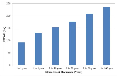
Figure 5.10: Storm Duration Sensitivity ... 67

Figure 5.11: Rainfall Event Occurrence Sensitivity ... 67

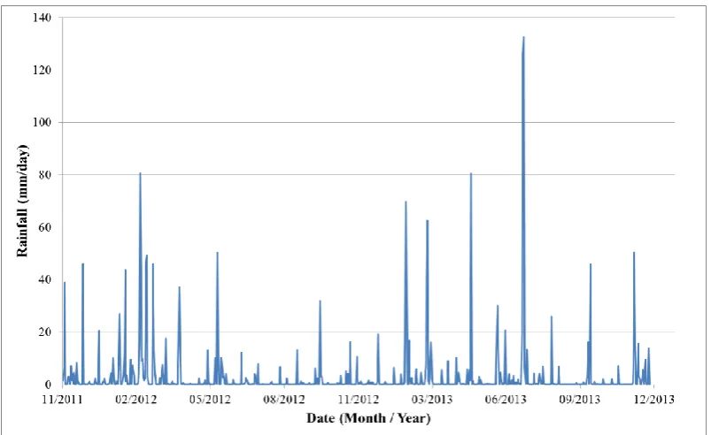
Figure 5.12: Daily Rainfall Nowra... 69

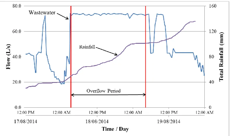
Figure 5.13: SPS 3 Overflow Event 16th to 18th August 2014 ... 72

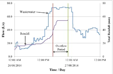
Figure 5.14: SPS 3 Overflow Event 25th to 26th August 2014 ... 74

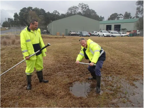
Figure 5.15: Submerged Manhole ... 75

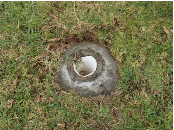
Figure 5.16: Broken inspection opening ... 76

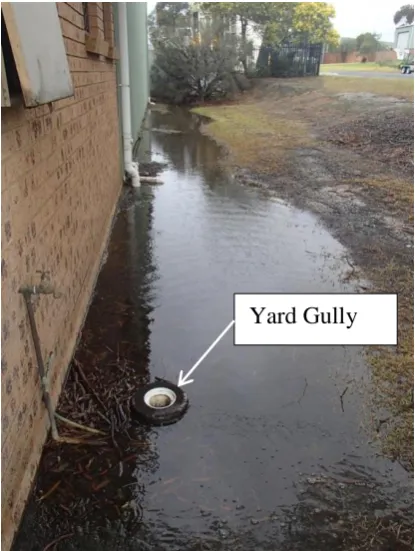
Figure 5.17: Yard gully inundation ... 77

Figure 5.18: Roof drainage connection ... 77

Figure 5.19: Manhole impacted by tidal inundation ... 78

Figure 5.20: Vertical Riser impact by tidal inundation ... 79

Figure 6.1: Overflow Relief Cap ... 85

Figure B.1: Overview of Nowra Sewerage Scheme ... 96

Figure H.1: SPS 15 SCADA Flow Data ... 107

Figure K.1: SPS 15 Diurnal Curve ... 131

Figure K.2: SPS 15 Diurnal Flow Variability ... 132

(14)

xiv

Figure K.6: SPS 26 Diurnal Flow ... 145

Figure N.1 - Field Work Catchment Plan 1 of 2 ... 160

(15)

xv

List of Tables

Table 2.1: No. of Water Utilities Serving 10,000 + customers ... 9

Table 2.2: ADWF Adopted Value Comparison ... 13

Table 2.3: Leakage Severity ... 19

Table 2.4: ARI Containment Factor ... 19

Table 2.5: Reduction of RDII for Public Sewer Rehabilitation ... 22

Table 3.1: Catchment Details ... 28

Table 3.2: Catchment 3 Gravity Pipeline Summary ... 28

Table 3.3: SPS Flow Delay Times ... 29

Table 4.1: Excel SCADA Data Format ... 35

Table 5.1: Maximum Inflow Times ... 45

Table 5.2: SPS 3 Dry Day Flow ... 46

Table 5.3: SPS 3 Dry Day Flow Expanded Data Set ... 47

Table 5.4: SPS 3 Monthly ADWF ... 48

Table 5.5: Comparison of ADWF methods. ... 49

Table 5.6: Peak Day ADWF SPS 3 ... 50

Table 5.7: ADWF Weekday / Weekend Summary ... 51

Table 5.8: Peaking Factors ... 54

Table 5.9: SPS 3 WSAA Dry Day Flow ... 57

Table 5.10: Minimum Flow ... 58

(16)

xvi

Table 5.12: Queensland Traditional PWWF Method ... 63

Table 5.13: SPS PWWF ... 68

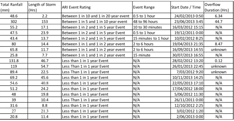
Table 5.14: Storm Event Rating and Duration ... 70

Table C.1: Water Utility and Design Standard Summary ... 97

Table F.1: Catchment 15 Pipeline Summary ... 104

Table G.1: Pump Performance and Identifier ... 106

Table J.1: SPS 3 Maximum Inflow Time... 116

Table J.2: SPS 3 Inflow Exceedance Days ... 117

Table J.6: SPS 21 Inflow Exceedance days ... 121

(17)

xvii

Table K.1: SPS 15 Dry Day Flow ... 128

Table K.2: SPS 15 Dry Day Flow Expanded Data Set ... 129

Table K.3: SPS 15 Monthly ADWF ... 129

Table K.4: SPS 15 WSAA Dry Day Flow ... 130

Table K.18: SPS 29 Dry Day Flow Expanded Data Set Analysis ... 147

(18)

xviii

Table L.2: Leakage Severity Sensitivity Calculations ... 155

Table L.3: Containment Standard Sensitivity Calculations ... 155

Table L.4: Sensitivity of Storm Duration Calculations ... 156

Table L.5: Sensitivity of Event Occurrence ... 156

(19)

xix

Glossary of Terms

A Area [ha]

AC Asbestos Cement

ADF Average Daily Flow [L/s]

ADWF Average Dry Weather Flow [L/s]

AHD Australian Height Datum [m]

ARI Annual Recurrence Interval

BOM Bureau of Meteorology

CCTV Closed Circuit Television

DWF Dry Weather Flow

EPA Environmental Protection Agency

EP Equivalent Population

ET Equivalent Tenement

GIS Graphic Information System

(20)

xx

IFD Intensity Frequency Duration

I/I Inflow / Infiltration

IO Inspection Opening

LGA Local Government Area

MF Minimum Flow [L/s]

MH Manhole

ML Mega litre

NSW New South Wales

PDF Peak Daily Flow [L/s]

PDWF Peak Dry Weather Flow [L/s]

PVC Polyvinyl Chloride

PWWF Peak Wet Weather Flow [L/s]

RDII Rainfall Dependant Inflow / Infiltration

SCADA Supervisory Control and Data Acquisition

(21)

xxi

SPS Sewer Pump Station

SSOAP Sanitary Sewer Overflow Analysis and Planning Toolbox

STP Sewer Treatment Plant

SW Shoalhaven Water

UPVC Unplasticised Polyvinyl Chloride

US EPA United States of America Environmental Protection Agency

VCP Vitrified Clay Pipe

VSD Variable Speed Drive

WSAA Water Services Association of Australia

(22)

1

Chapter 1: Introduction

Sewer system networks are designed on the basis of estimating the expected discharge from a catchment that has a variety of land uses. These land uses include residential, commercial and industrial which all have a variety of activities that are undertaken. Historical metered water records provide an indication into the types of water uses that may be occurring and from this an estimated discharge of wastewater can be approximated.

To enable a desktop analysis to be undertaken an assumption is made to the Equivalent Population (EP) of the area. The equivalent population is related to the discharge of a single person in a standard residential home, and the equivalent population in a home is known as an Equivalent Tenement (ET). Historical evidence has enabled a statistical relationship to be determined for the EP/ET of commercial, industrial and medium to high density residential living. This evidence needs to be correlated to localised conditions and occupancy rates.

The population estimates used to determine the catchment loading provides an indication of the expected Average Dry Weather Flow (ADWF). This flow is the average flow that is expected to occur on a normal dry day over a 24 hour period. Actual flows during this period however will vary and peaks of high discharge to wastewater will be evident, the peak flow is known as Peak Dry Weather Flow (PDWF). In a residential home these peaks are evident in the morning and afternoon as residents use the homes facilities to wash, shower etc. The diurnal curve for other land uses however is different from that of a home; the result is each catchment will develop its own unique characteristic diurnal curve.

(23)

2 usually 30 years, to allow for growth in the catchment without needing to augment the system.

Experience has also shown that it is not possible to develop a wastewater system that is not susceptible to inflow or infiltration from either rain water or groundwater. Pressure sewer systems in recent years are reducing the impact through the use of continuous pipe however illegal stormwater connections and leaking toilets and taps are still present.

It is only once a system has operated for a period of time that the true flow characteristics can be determined. These characteristics will also change with time as the catchment grows and land use/habits change. For this reason it is important for wastewater system operators to monitor flow trends and plan for system augmentation prior to the system reaching the ultimate design flow.

Rainfall Derived Inflow and Infiltration (RDII) can drastically reduce the hydraulic capacity of a system, whilst removal of a portion of RDII can extend the hydraulic life span of the system and thus delay expensive augmentation works. Once the hydraulic capacity of a system is exceeded overflows shall occur, these overflows can affect the health of the local environment. In recent years there has been a move by the industry to analyse the system based on the local climatic conditions and to ensure that system capacities are capable of dealing with the majority of rainfall events.

To enable the management of the system it is important for operators to monitor and manage the flows within catchments. When flows are exceeding expectations investigations need to be undertaken to determine the cause. As the largest flow contributor to the hydraulic capacity of the system is the PWWF, a reduction in this component of flow can represent the largest reduction in flows to maintain capacity. Thus the need for development of a strategic approach that enables both short and long term abatement programs to be implemented successfully.

(24)

3 ADWF/PWWF periods. These hydrographs enable the identification of excess wet weather flows as either inflow (immediate impact) or infiltration (delayed impact). Good Practice guidelines and previous case studies that have been published outline operator’s attempts to identify and rectify I/I. These case studies outline the process undertaken and also the methods used to mitigate the I/I. This experience allows a more informed and cost effective management plan to be established from the lessons learnt by others.

As with all strategic plans it is important to also develop methods to measure the effectiveness of mitigation methods used to reduce the I/I.

1.1.

Background

The Shoalhaven Region is located on the South Coast of New South Wales, approximately 160km south of Sydney. The Shoalhaven City Council (SCC) Local Government Area (LGA) is 4660km2 in size, approximately 120km long (North/South) and 80km wide (East/West). It encompasses 19 major waterways, including Jervis Bay, St Georges Basin, Crookhaven River and Shoalhaven River. Nearly 70% of the Shoalhaven is national park, state forest or vacant land. The region has 2 major centres being Nowra/Bomaderry in the north and Milton/Ulladulla in the south. A number of small townships and settlements make up the remainder of the urban areas (SCC, 2010).

It has a permanent population of approximately 85,000 people with a peak population in excess of 275,000 people during peak tourist periods. Shoalhaven Water (SW), a division of SCC, currently operates 13 wastewater schemes within the Shoalhaven Local Government Area.

The main employment sectors are summarised as follows • Agriculture: Dairy and Oyster Industry

(25)

4 • Government agencies: Local and State government including the South Nowra Correctional Facility

• Health: Including a number of retirement villages, 1 large hospital and various smaller facilities.

• Manufacturing: Australian Paper Mill, Manildra ethanol processing and facilities servicing HMAS Albatross

• Tourism: A number of coastal areas have large tourist facilities, mainly caravan parks.

The 13 wastewater schemes are located at Berry, Bomaderry, Bendalong, Callala Bay, Culburra, Huskisson/Vincentia, Kangaroo Valley, Lake Conjola, Nowra, St Georges Basin, Shoalhaven Heads, Sussex Inlet and Ulladulla.

(26)

[image:26.595.118.518.74.658.2]

5 Figure 1.1: Shoalhaven Local Government Area (LGA)

(27)

6 Each sewerage system is designed to service the urban area of the various townships. The treated effluent from the treatment plants discharges to either the Ocean or Shoalhaven River. Reuse systems are in operation for 6 of the schemes, with the treated effluent reused on farmland. The Shoalhaven River and Crookhaven River in the north are connected with a large oyster industry located in the lower reaches of both rivers. Nowra and Bomaderry Sewer Treatment Plants (STPs) are licenced to discharge to the Shoalhaven River. Shoalhaven Heads and Culburra STPs are both in close proximity to the oyster leases and have a reuse scheme for discharge of their treated effluent. In the event of untreated effluent escaping to the local environment in these urban areas the impact can result in the closure of recreational and commercial activities due to potential impacts on health.

The 3 sewerage schemes servicing the townships of Lake Conjola, Bendalong and Kangaroo Valley have been commissioned in the past 7 years. These schemes were undertaken to improve the social amenity of the local area as the townships were serviced by either septic tank or onsite disposal systems.

The Nowra sewerage scheme was originally commissioned in 1937 and augmented as the township grew. A point has now been reached which requires major augmentation of both the Nowra and Bomaderry sewerage treatment plants. This will require a large capital investment in excess of $100 million dollars. The intent of the upgrade is to ensure that the communities of Nowra and Bomaderry are able to be serviced for the next 30 year horizon. Appendix B – Overview of Nowra Sewerage Scheme shows the general arrangement of the Sewer Pump Stations (SPSs) and STP in Nowra.

1.2.

Problem Identification

All of the sewerage schemes within the Shoalhaven region are impacted upon by I/I to various extents. During wet weather events the hydraulic capacity of several SPS’s and STP’s is exceeded. At present no overall strategy exists to identify and rectify the issue, the impact of I/I includes

(28)

7  Impact on the local environment,

 Complaints from local residents,

To enable future planning and management of the wastewater system/s a strategy is needed to

 Identify resources required to identify problematic catchments,

 Review past practices and effectiveness of studies undertaken in the Shoalhaven region,

 Determine the impact and frequency of the events,

 Utilise best practice guidelines for the establishment of the strategy,

I have chosen this project as my current role of Wastewater Operations Manager requires me to operate and maintain the various sewer systems that Shoalhaven Water is responsible for. As part of this management I need to ensure that a strategic approach is developed to deal with operational issues. This strategic approach will enable a more efficient and effective use of resources, allow forward planning of system augmentation and ensure that compliance with environmental licence conditions is maintained.

(29)

8

Chapter 2: Literature Review

The literature review has been undertaken in two (2) parts the first being the review of Standards used for the calculation of hydraulic capacity and the second being a review of case studies for the short and long term abatement of inflow and infiltration.

2.1.

Review of Sewer Design Standards

An extensive review of the adopted design practices by Australian water utilities has been undertaken to determine the current practices used for the design and operation of sewerage systems. The Water Services Association of Australia (WSAA) currently has 2 codes that “sets out to provide guidance by way of general principles, criteria and good practice” (WSAA, 2004). These codes were originally released in

1999 with the current versions being

 Sewerage Code of Australia WSA 02-2002 Second Edition Version 2.3,  Sewage Pumping Station Code of Australia WSA 04-2005 Second Edition

Version 2.1

The introduction and release of these codes enabled a common approach for Australian water utilities to plan, design, construct and operate sewerage systems. The past practices of water utilities have been to utilise a number of methods and criteria to determine hydraulic capacity. In 1989 at the 13th Federal Convention of Australia Water and Wastewater Association, the manager for planning at the Water Board Sydney noted that

“A survey of national design criteria has shown that there is not only a range of methods in use for determining sewer hydraulic capacity but a wide scatter of design allowance. This variation appears to be greater than the variation in prevailing climatic, geographic and geological conditions”

(30)

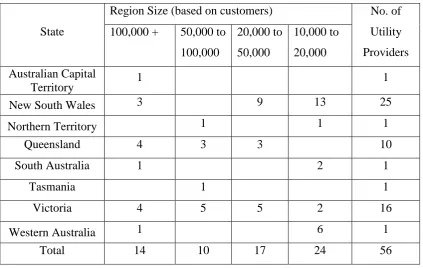
9 In Australia there are 65 sewer utilities providing sewerage services to a population of 10,000 or more people. Each of these utilities sets its own design standards for their respective systems.

[image:30.595.108.532.310.578.2]

Table 2.1 - Water Utilities serving 10,000 or more customers is a summary of the number of utilities and the population groups that they service. Australian Capital Territory, Northern Territory, South Australia, Tasmania and Western Australia have only one sewer service provider whilst New South Wales has 25. Each service provide however may operate a number of regions which then control a number of wastewater schemes.

Table 2.1: No. of Water Utilities Serving 10,000 + customers

State

Region Size (based on customers) No. of Utility Providers 100,000 + 50,000 to

100,000 20,000 to 50,000 10,000 to 20,000 Australian Capital

Territory 1 1

New South Wales 3 9 13 25

Northern Territory 1 1 1

Queensland 4 3 3 10

South Australia 1 2 1

Tasmania 1 1

Victoria 4 5 5 2 16

Western Australia 1 6 1

Total 14 10 17 24 56

(Source National Water Commission 2014)

Note: This summary excludes Melbourne Water which is a bulk water utility.

(31)

10 Other standards are also still being used. A summary of the standards is as follows;

 WSA 02-2002 Sewerage Code of Australia Version 2.3.

 WSA 02-2002 Sewerage Code of Australia Sydney Water Edition Version 3.  WSA 02-2002 Sewerage Code of Melbourne Retail Water Agencies Edition

(MRWA) Version 1.0.

 WSA 02-2002 Sewerage Code of Australia Hunter Water Edition.  NSW Public Works Manual of Practice Sewer Design (1984).

 Aus –Spec Development Design Specification D12 Sewerage System.

 Metropolitan Water and Sewerage Drainage Board - Sydney Manual Design. of Separate Sewer Systems (1979).

 Queensland Planning guidelines for water supply and sewerage 2010.

The majority of the utilities that adopted the WSSA sewerage code also had supplements to the design code for local variations. In NSW some utilities used more than one code, whilst in Queensland the traditional method as outlined in the planning guidelines is also used by smaller utilities i.e. Calliope Shire Council. In Victoria there was a consistent approach across all utilities to utilise the same standard whilst in the Northern Territory the standard specified is the 1979 edition of the now Sydney Water Board. It is also important to note in NSW that the three (3) Water Authorities being Sydney Water, Hunter Water and the recently formed Central Coast Water Corporation have individual legislation for their operation, whilst the remaining water utilities are under the management of the local Councils and the NSW Office of Water.

(32)

11

2.2.

Hydraulic Capacity

The basis of all design criteria is to determine a design flow to ensure hydraulic capacity of the system is adequate; the following definitions are used in the determination of the design flow.

Average Dry Weather Flow (ADWF): The combined average sanitary flow into a sewer from domestic, commercial and industrial sources.

Design Flow: The estimated maximum flow into a sewer comprising the sum of peak dry weather flow (PDWF), ground water infiltration (GWI) and stormwater inflow and infiltration (IIF) (WSAA, 2002).

Equivalent Population (EP): The equivalent hypothetical residential population that would produce the same peak dry weather flow as that contributed by the area under consideration i.e. all zonings including residential, commercial and industrial. For a single residential dwelling the occupancy rate adopted is 3.5 (WSAA, 2002). Examples of EP for different zonings have been provided in Appendix D – Sewer Design Code Equivalent Populations for Synchronous discharges.

Equivalent Tenement (ET): This value is the equivalent residential houses that would produce the same ADWF as that contributed by the area under consideration i.e. all zonings including residential, commercial and industrial. A local occupancy rate can be used to determine the EP. Appendix E – Water Directorate NSW Standard ET

Groundwater Infiltration (GWI): is caused where the long-term non-rainfall dependent groundwater table or seawater level exceeds pipe invert and enters the sewer network (WSAA, 2002).

Inflow/Infiltration (I/I): This is the peak (rainfall dependant) inflow and infiltration that may enter the sewer network as inflow via illegal stormwater connections or localised flooding of yard gullies and as rainfall infiltration through pipe and maintenance structure defects (WSAA, 2002)

(33)

12 Based on the above definitions the design flow, also known as the Peak Wet Weather Flow (PWWF) is able to be calculated as follows:

Design Flow (PWWF) = PDWF + GWI + IIF (2.1)

2.3.

Average Dry Weather Flow

The estimation of ADWF can either be done by flow monitoring or empirical estimation. In existing systems, where practical, flow monitoring is undertaken to establish the flow characteristics of the catchment. Where it is not possible to physically gauge the flow in a system the empirical method can be used. For new growth areas (land subdivision) the empirical method is adopted to determine the estimated flow.

The empirical method requires the establishment of an estimated flow per person, this value is then multiplied by the EP of the catchment to determine the ADWF of the catchment. “Based on empirical evidence, ADWF is deemed to be180L/EP/d or 0.021 L/s/EP”(WSAA, 2002).

In Queensland the “Planning Guidelines for Water Supply and Sewerage 2010”

notes that “generally ADWF will range from 150-275 L/EP/d” (Queensland Water

Supply Regulator, Water Supply and Sewerage Services, Department of Energy and Water Supply).

In NSW the Water Directorate notes that “Average dry weather sewage rates generally lie between 0.004 L/s/ET and 0.011 L/s/ET. It is generally accepted that a sewer ET represents an average loading of around 0.008 L/s at both state and local level with the accepted design value being 0.011 L/s/ET” (Water Directorate, 2005).

The NSW Public Works recommended at design value of 0.011 L/s/ET (NSW Public Works, 1984). In 1994 the NSW Public works department recommended a value of 240L/EP/d (NSW Office of Water, 2012).

(34)

13 In non-metropolitan NSW the NSW Office of Water recommends an ADWF value of 200 L/EP/d be adopted. This value represents a 75% sewer discharge factor for the 250kL/annum medium residential water supplied per connected property for inland utilities. This value represents a typical occupancy rate of 2.6 persons per house (NSW Office of Water 2012). Sydney Water has adopted a value in line with WSAA of 180L/EP/d, the average water consumption in Sydney is 623L/ET/d.(Sydney Water, 2014).

When flow monitoring of the catchment is undertaken to determine ADWF the flow will consist of domestic wastewater and GWI, the GWI can be determined as the flow that occurs during the early morning hours i.e. 12am to 4am (USQ, 2011). In summary the ADWF as adopted by WSAA of 180L/EP/d is within the ranges recommended both in Queensland and NSW. Local assessment of the ADWF, where possible, should be undertaken to ensure consistence with internal water usage. This can be done by either calibration of metered water usage with measured sewer treatment plant (STP) flows or flow monitoring. Table 2.2 – ADWF Adopted Value Comparison summarises the variations noted above.

Table 2.2: ADWF Adopted Value Comparison

Authority ADWF (L/EP/d)

Water Service Association of Australia 180

Water Directorate (NSW) 99 - 271

Department of Energy and Water (QLD) 150 - 275

Public Works (NSW) 240

Office of Water (NSW) 200

(35)

14

2.4.

Peak Dry Weather Flow

The PDWF can be related to the ADWF by a peaking factor (d).

PDWF = d x ADWF (2.2)

The WSAA sewer code relates the peaking factor to the gross development area. The value of d can be calculated using the following formulae;

d = 0.01(log A)4 – 0.19(log A)3 + 1.4(log A)2 – 4.66(log A) + 7.57 (2.3) ‘A’ is the gross plan area of the development catchment, in hectares. This relationship may be used for catchments up to 100,000 hectares.

The NSW Public works adopt a different method for the calculation of the peaking factor; this factor is denoted ‘r’ in the 1984 sewer design standard and uses the no. of tenements (T) for the calculation.

𝑟 = √ 1.74 + _𝑇56_0.4 𝑓𝑜𝑟 𝑇 > 30 (2.4)

The historical Queensland approach adopted a different method for the calculation of peaking factor, this factor is denoted ‘C2’ and uses the EP for the calculation

C2 = 4.7 x (EP)-0.105 (2.5)

(Queensland Water Supply Regulator, Water Supply and Sewerage Services, Department of Energy and Water, 2010)

(36)

15 Figure 2.1: Comparison of PDWF Peaking Factors

Note: NSW Public Works is based on ET’s, Queensland traditional method is based on EP, and an occupancy rate of 3.1 has been applied to determine ET. The WSAA method uses area.

A discrepancy between peaking factors is still evident at 500 ETs, this difference results in a variation in the calculated PDWF. The Queensland method uses the EP of a residential home whilst the Public Works method uses equivalent tenements to calculate the peaking factor. In NSW an ET is based on 2.6 EP which is lower than the Queensland adopted value of 3.1EP thus if 2.6 EP was used the Queensland peaking factor would be closer to that of the other two peaking factors shown.

(37)

16 Figure 2.2: Residential Diurnal Curve

(Source Shoalhaven Water Flow Monitoring Records)

Figure 2.3 – Industrial Estate Daily Flow Variation shows the diurnal pattern for wastewater discharge in an industrial area. This curve indicates one peak in the 24 hour period showing a consistent wastewater discharge during the hours of operation.

(38)

17

2.5.

Peak Wet Weather Flow

Three methods for calculating PWWF are shown below 1. NSW Public Works Method

PWWF = PDWF + SA (2.6)

Where SA = Storm Allowance [0.058 L/s/ET] 2. Queensland Traditional Method

PWWF = 5 x ADWF or (2.7)

PWWF = C1 x ADWF (2.8)

Where C1 = 15 x (EP)-0.1587 (Note C1 Minimum = 3.5)

3. WSAA Method

PWWF = PDWF + GWI + I/I (2.9)

Where GWI = Groundwater infiltration [L/s] I/I = Inflow/infiltration

The calculation of ground water infiltration, using WSAA, is done using the following formulae

GWI = 0.025 x A x PortionWet (2.10)

Where A is the gross plan area of the developments catchment, in hectares. PortionWet is the portion of the planned pipe network estimated to have

groundwater tables in excess of pipe inverts. For example if 70% of the sewer system is below groundwater table levels, then PortionWet = 0.7.

(39)

18

areas, the potential for 24 hour industries and automatic urinal flushing needs to be taken into account” (WSAA, 2011).

The WSAA method for calculating inflow/infiltration is as follows

IIF = 0.025 x AEff x C x I (2.11)

AEff is the effective area capable of contributing rainfall dependant

infiltration. For residential developments AEff is a function of the

development density

AEff = A x (Density/150)0.5 for Density < 150 EP/ha (2.12)

AEff = A for Density > 150 EP/ha (2.13)

Where A is the gross plan area of the developments catchment, in hectares. Density is the developments EP density per gross hectare.

For commercial and industrial developments AEff is a function of the

expected portion of the catchment to be covered with impervious structures, i.e. roofs, sealed roads, car parks.

AEff = A x (1 – 0.75 PortionImpervious) (2.14)

Where A equals the gross plan area of the developments catchment

PortionImpervious equals the portion of the gross plan area likely to be

covered by structures that drain directly to the stormwater system i.e. 20% = 0.2.

C equals the leakage severity co-efficient and it defines the contribution of rainfall run-off to sewer flows. It is the sum of contributions from soil movement and network defects.

(40)

19 Table 2.3: Leakage Severity

Leakage Severity Co-efficient (C)

Influencing aspect Low Impact High Impact

Soil aspect, Saspect 0.2 0.8

Network aspect, Naspect 0.2 0.8

C = Saspect + Naspect Min = 0.4 Max = 0.8

(Source WSAA, 2002)

I is a function of rainfall intensity at the developments geographic location, catchment area and required sewer system containment standard.

I = I1,2 x FactorSize x FactorContainment (2.15)

I1,2 is the 1 hour duration rainfall intensity at the location, for an average

recurrence interval of 2 years.

FactorSize accounts for the faster flow concentration times in smaller

catchments.

FactorContainment reflects local environmental aspects and regulations on wet

weather sewerage containment (overflow frequency).

The design should incorporate the Average Reoccurrence Interval (ARI) of sewage overflow, which is adopted by the water agency. Given a specified ARI, FactorContainment may be either taken from Table 2.4 or calculated as follows:

𝑭𝒂𝒄𝒕𝒐𝒓_{𝑪𝒐𝒏𝒕𝒂𝒊𝒏𝒎𝒆𝒏𝒕} = 𝟎. 𝟕𝟕 𝒙 𝟏𝟎𝟎.𝟒𝟑𝑿

𝟏𝟎𝟎.𝟏𝟒𝑿𝟐 (2.16)

Where X = Log10 (ARI) and ARI is the specified containment in years.

Table 2.4: ARI Containment Factor

ARI 1 month 3 month 6 month 1 year 2 years 5 years 10 years Factor

(Containment)

0.2 0.4 0.6 0.8 1.0 1.3 1.5

(41)

20 After a review of the NSW Public Works sewer design manual and discussion with other engineers in the workplace, it was uncertain how the value of 0.058 L/s/ET has been derived. Advice from Manly Hydraulics Staff (a division of NSW Public Works) is that the value was adopted as the maximum metered water usage of a standard residential household in the late 1970’s (Dakin, SK, 2014 pers. comm 2nd

August). Whilst the storm allowance does allow for ease of calculation in essence this value has no relationship to actual rainfall derived I/I nor does it take into account climate variation across different regions of NSW.

There is evidence of Councils in NSW modifying the storm allowance. Shoalhaven City Council (SCC) is currently using two storm allowances with SA = 0.058 L/s/ET for old areas and 0.030 L/s/ET being adopted for new works (SCC, 2013). Wagga Wagga City Council (WWCC) adopted a storm allowance of 0.029 L/s/ET. WWCC noted that this was 50% of the NSW Public Works value (WWCC, 2013) and justified the reduction with a comparison of rainfall data between Wagga Wagga and Sydney.

There was evidence of a simple empirical method of calculating PWWF by multiplying ADWF by a factor. This method appears to have been used historically as it was difficult to quantify Rainfall Derived Inflow and Infiltration (RDII). The Sydney Metropolitan Drainage Board used 6 x ADWF for pump station and 8 x ADWF for sewers (Dunning, 1958). This method was justified in 1958 for the design of the Wellington (New Zealand) Pumping Station which was based on a maximum flow of 230 gal/head/day, being 6 times the ADWF (Dunning, 1958). This method is still used by utilities today with Byron Bay Council adopting PWWF = 7 x ADWF as a standard to be met for its level of service (Byron Bay Council, 2013).

2.6.

Review of Inflow / Infiltration Case Studies

(42)

21 In the 1960’s flexible jointed sewers were introduced and the flexible joint was extended to property service connections in Melbourne in 1973 (Barnes et al, 1975). This was an attempt to reduce the impact of infiltration by the use of improved construction materials.

In 1975 it was noted that the Melbourne sewerage system was impacted upon by I/I. This impact was a result of

 Groundwater infiltration via fractured pipes and joints  Wastewater from leaking fittings

 Stormwater inflow from illegal connections  Flooding at manhole covers.

It was noted that allowances had been made at the design stage with the existing system commissioned 77 years early and that increase in dry weather flows had taken up capacity and thus these allowances for I/I had been reduced. An infiltration steering committee was assigned the responsibility of reviewing current practices and modifying design and construction methods to minimise infiltration (Barnes Et al, 1975).

The Sydney Water Board detailed in 1992 its sewer gauging strategy that had been developed on 10 years of historical gauging data. The intent of the strategy was to significantly reduce the main sources of I/I by:

 Identifying areas which contribute to most of the problem  Use accurate computer modelling of the system

 Plan and measure the effectiveness of remedial work  Enable management of the entire sewer network

(43)

22 A recent guideline, “Management of Wastewater System Infiltration and Inflow Good Practice Guideline” released by WSAA (2013) concluded that unless at least

40% of the total piped system within a catchment is rehabilitated there is no guarantee of reducing RDII. Table 2.5 – Reduction of RDII for Public Sewer Rehabilitation summaries WSAA findings.

Table 2.5: Reduction of RDII for Public Sewer Rehabilitation % of Total Public System

Rehabilitation

Reduction in RDII (%) Reduction in GWI (%)

100 60 +/- 80

80 40 +/- 70

60 20 +/- 50

40 0 +/- 30

(Source WSAA, 2011)

North Shore City Council (New Zealand) rehabilitated 32 catchments over a 10 year period. They discovered that two (2) variables could be used to provide a prediction of the reduction of RDII% and PWWF. The two variables were the percentage of total network (private and public) rehabilitate and the initial leakiness of the system (RDII%). This lead to the development of the following 2 equations (WSAA, 2013)

RDII% = Initial RDII factor x Percentage complete (2.17) = (0.257 Ln (-0.0445x + 0.0445 + RDIIpre) + 0.988) * X1.055

Peak Flow % reduction = Initial RDII factor x percentage complete (2.18) = (0.303Ln (-0.0445x + 0.0445 + RDIIpre) + 1.163) * X0.761

WSAA noted that the above has not been calibrated in Australia to date due to insufficient I/I analysis.

(44)

23 From seven case studies reviewed by WSAA (WSAA, 2011) it was determined that the following steps should be followed in the establishment of an I/I abatement strategy:

 A survey to quantify major inflow will need 3 to 4 storms of significant wet weather events,

 There is a near proportional relationship between rainfall depth and inflow,  Effective management of data i.e. SCADA to enable ready interface with

analysis platforms,

 Calibrate the hydraulic model for dry weather flow,  Calibrate for wet weather flow,

 Verify the model,

 Undertake an Options Assessment,  Develop a remediation plan,  Implement remediation plan,  Benefits realisation review,

The remediation plan can consider a number of options that includes, maintenance hole inspection, smoke testing, dye testing, CCTV and data management of inspections.

All of these abovementioned remediation works are currently undertaken, to varying extent, by Shoalhaven Water. The relining of the pipe network that has been completed appears to have minimal impact on I/I.

The U.S Environmental Protection Agency (US EPA) in 2009 released its first version of the Sanitary Sewer Overflow Analysis and Planning Toolbox (SSOAP). This toolbox was developed by the EPA and CDM Inc. and has been effective in sewer condition assessment and rehabilitation to support wastewater system improvements (US EPA, 2012).

(45)

24 software has been made available in the public domain free of charge with the intended user to be wastewater system operators. The intent of this is in the interest of the community and to remove the cost prohibition that commercial software can be for smaller organisations to undertake an analysis.

The software is available at http://www.epa.gov/nrmrl/wswrd/wq/models/ssoap/. WSAA has also recently released an excel toolkit for analysing SCADA pump run time data, this toolkit also produces hydrographs. A paper on the WSAA Good Practice Guideline for the management of Wastewater system infiltration and inflow was discussed at the Ozwater conference in April 2014 (paper 26).

A copy of this software does not appear on the WSAA website however WSAA have been contacted to obtain a copy of the software.

2.7.

Conclusion

The current sewer design practice as set out by WSAA in its sewer design code of Australia is the most suitable method for estimating flow parameters. This method utilises actual system performance via flow monitoring and determines the flow components in relation to the local climatic conditions for a known ARI. This method follows Best Practice Guidelines and provides a degree of certainty to the actual performance of the system during a wet weather event.

Utilising the SSOAP toolbox or the WSAA toolkit will enable an I/I analysis to be undertaken using existing SPS SCADA records and Bureau of Meteorology (BOM) rainfall data. The hydrographs will provide an indication as to whether the majority of the problem is a result of Inflow or Infiltration.

A comparison of the PWWF value that has been adopted by Shoalhaven Water, using the traditional method, will also be compared to the PWWF determined by the WSAA method. This will determine if the existing system is exceeding design capacity as a result of local climatic rainfall conditions.

(46)

25 analysis will be undertaken during wet weather events and is reliant on suitable rainfall occurring during the investigation period.

The strategy for the management of I/I will be developed taking into account the ease of desk top analysis and the success / failure of the field analysis. Rectification measure to mitigate I/I will be developed and suggestions for improvements to the design guidelines will be made.

(47)

26

Chapter 3: Overall Aim and Objectives

The Nowra sewerage scheme has a permanent population of 29,400 people with minimal tourist population. The scheme consists of a number of catchments that transfer effluent via gravity to sewer pumping stations (SPSs) or direct to Nowra Sewer Treatment Plant (STP). The Nowra Scheme consists of 29 SPSs and 210km of gravity sewer mains. One catchment within this scheme shall be used as a project site for analysis.

3.1.

Project Site

The Project site is one catchment from the Nowra scheme; this catchment is the St Ann’s St Catchment. This catchment transfers effluent via a SPS, known as SPS 3. It consists of multiply land uses including residential, commercial and industrial. In addition the catchment also has 5 SPSs discharging to the gravity network.

The 5 SPS’s and their land uses are summarised as follows

 SPS 15: Residential and receives pump flows from 2 upstream SPSs including HMAS Albatross industrial services,

 SPS 21: Residential with a large integral energy complex,  SPS 23: South Nowra Industrial precinct,

 SPS 26: University of Wollongong southern campus,  SPS 29: South Nowra Correctional Facility.

Figure 3.1 – St Ann’s St Catchment overview shows the location of SPS 3, the main trunk gravity mains (shown blue) and the 5 SPS’s (15, 21, 23, 26 and 29) that discharge into the trunk gravity system. The rising mains for the SPS’s are shown in red.

(48)

27 System (GIS) shall be utilised for the location and size of the sewer infrastructure as part of the field analysis.

During wet weather events, the St Ann’s Street catchment is heavily impacted by I/I, SPS 3 and manholes within the gravity system draining to the SPS overflow during these events.

Figure 3.1: St Ann's St Catchment Overview (Source: Shoalhaven Water, 2013)

3.1.1. Catchment Properties

(49)

28 that the ET’s shall be fixed for the adopted analysis period of 3 years. Table 3.1 – Catchment details is a summary of the catchments population and area.

Table 3.1: Catchment Details SPS Catchment Equivalent Tenements (ET) Equivalent Population (EP) Catchment Area (ha)

3 1263 2993 199.7

15 154 365 68.6

21 234 555 29.6

23 37 88 22.1

26 9 21 2.9

29 253 600 3.0

3 (All) 1950 4622 325.9

3.1.2. Sewer Network

The sewer network consists of extensive gravity mains with upstream catchments connecting via rising mains from each of the respective SPS’s. Within catchment 3 there is 27.4km of gravity mains ranging in size from 150mm up to 450mm with a short section of 600mm main connecting the network to SPS 3. Table 3.2 – Catchment 3 Gravity Pipeline Summary provides details of the type of pipe, size, age and lengths installed.

Approximately 17.4km of this network consists of either Asbestos Cement (AC) or Vitrified clay pipe (VCP). 90% of the gravity pipes have been operating for 25 or more years.

Table 3.2: Catchment 3 Gravity Pipeline Summary

5 10 15 20 25 30 35 40 45 55

150 65 1393 2307 3764

225 406 528 934

300 732 1064 1796

450 498 2979 3478

150 327 131 2340 2345 1472 6615

225 32 404 436

UPVC 150 360 1552 1013 52 2977

150 6500 6500

225 877 877

600 15 15

DICL 150 50 50

360 1552 1340 131 2372 2345 3174 6419 2356 7392 27441

Total Length (m) AC/C PVCP VCP Total (m)

Pipe Length (m) / Age (Yr's) Pipe Size (mm)

(50)

29 Details of the gravity pipelines for the upstream catchments are provided in Appendix F – SPS Gravity Pipeline Summary.

3.1.3. Upstream SPS Flow Transfer Times

The upstream sewer catchments transfer pumped flows to catchment 3 via rising mains. The velocity of flow in each rising main has been adopted from SW’s records to enable an estimated time to be calculated for the flow to reach the gravity catchment. The length and grade of the gravity mains that transfer each of the pump flows to SPS 3 has been adopted from SW’s records. A velocity of 1m/s has been adopted for the pumped flows within the gravity section. The basis for this is no hydraulic modelling of the network flows has been undertaken, however field measurements at various points in the network, during dry weather, indicate that this value is reasonable. Table 3.3 – SPS Flow Delay Times summaries the total delay for each SPS that has been adopted. It can be seen that the flows from SPS 21 arrive at SPS 3 after 30 minutes whilst the flows from the jail take approximately 115 minutes.

Table 3.3: SPS Flow Delay Times

These delay times are taken into consideration for the calculation of flows within catchment 3. Each delay time is rounded to the nearest 5 minute period for the purpose of developing the diurnal curve for catchment 3’s gravity section.

SPS 15 21 23 26 29

M.H Discharge I.L 54.34 28.95 54.34 50.033 35.7

SPS Inlet I.L 13.425 13.425 13.425 13.425 13.425

Length Of Main 4005 1560 4005 2356 3202

Gravity Grade 1.02% 1.46% 1.02% 0.97% 0.83%

Velocity 1 1 1 1 1

Travel Time (Gravity) 4005 1560 4005 2356 3202

Rising Main Length 402.5 443 474 1484 1869

Velocity 0.6 1.7 1.7 0.5 0.5

Travel Time (Rising Main) 671 261 279 2968 3738

(51)

(52)

31

3.2.

Project Overview

The intent of the project is to develop a strategy to be used throughout the Shoalhaven region to identify and rectify I/I issues. At present no overall strategy exists and different approaches have been utilised to at least address the impacts. Whilst the project is not intended to solve the issue of inflow and infiltration it will provide the framework to develop a systematic approach to managing and maintaining the wastewater system. It will enable Shoalhaven Water to prioritise future works, including maintenance and capital programs, taking into account the severity and risk associated with the impacts of inflow and infiltration.

The project will use the following steps to develop the strategy

1. Utilise the literature review on the design guidelines from various states and use 3 common design methods to estimate PWWF.

2. Use the knowledge learnt from other studies to customize the I/I values that suit the local conditions.

3. A problematic catchment within Shoalhaven wastewater network (SPS 3 – Nowra) shall be investigated using baseline data of ADWF during dry days, rainfall events and corresponding PWWF for the catchment.

4. A methodology will be developed for field analysis of the problematic catchment.

5. A Trial investigation during a wet weather event (subject to wet weather) using the developed methodology in 4 shall be carried out.

6. The field results will be analysed to determine if the field methodology was successful in identifying the primary source of I/I causing pump station / manhole overflows during wet weather.

(53)

32 8. Suggested improvements to the design guidelines based on the gather data and

field investigation shall be made.

3.3.

Conclusion

(54)

33

Chapter 4: Project Methodology

The project has been based on a 3 year period, from April 2011 to April 2014. This period has been adopted as a new pump station, SPS 29, was commissioned in July 2010 to service a correctional facility. Based on operational knowledge of SPS 29 the correctional facility was fully operational by January/February 2011.

4.1.

Existing Flow

The existing daily flow profile from SPS 3 and the 5 contributing upstream catchments is calculated using the Shoalhaven Water historical records. These records are based on the SPS “Supervisory Control and Data Acquisition” (SCADA) system. These records contain the pump run times for each SPS (with time steps) and this data has been extracted from the system and exported into Excel. The average flow between pump runs is calculated using the pump flow rates from Shoalhaven Waters draw down test records. The drawdown tests were completed in 2012 by Shoalhaven Water staff.

For SPS 3 there are two pumps which operate as duty and standby, these pumps also operate at either low speed or high speed depending on the rate of incoming flow. The five upstream pump stations have single speed pumps that operate as either duty/standby or combined. The pumps are regularly rotated from duty to standby. The details for each SPS pump performance and associated identifier is provided in Appendix G – SPS Pump Performance and Identifier.

4.2.

Excel Processing

The SCADA data is imported to Excel to enable a flow file to be created. The average flow in a time period is calculated on the basis that inflow occurs from the time the pump stops through to the next time the pump stops after a pump run. The outflow is the volume of effluent pumped whilst the pump is running

Average Flow = Pump Flow Rate x Time of Pumping

(55)

34 Figure 4.1: Average Flow per Period of Time illustrates equation 4.1, the period of time that the pump is off / on constantly varies. When high inflow periods are experienced for SPSs with dual speeds the pumped flow increases accordingly as shown in inflow period 2 in Figure 4.1.

Figure 4.1: Average Flow per Period of Time

This calculation is repeated for the analysis period of 3 years for SPS 3 and the five upstream SPSs. The following values are then calculated for each day.

 Average Day Flow (ADF),  Peak Day Flow (PDF),  Minimum Flow (MF).

Using the calculated values for all SPSs the gravity catchment flows for SPS 3 are as follows;

ADF Catchment 3 = ADF (SPS 3) – ADF (SPS 15) – ADF (SPS 21) – ADF

(SPS 23) – ADF (SPS 26) – ADF (SPS 29) (4.2)

PDF Catchment 3 = PDF (SPS 3) – PDF (SPS 15) – PDF (SPS 21) – PDF

(56)

35 A check of the time period when each peak day flow occurs at each SPS will need to be taken to ensure that the peaks occur during a similar time period. This will also need to take into account an approximate travel time for the flows to reach SPS 3.

MF Catchment 3 = MF (SPS 3) – MF (SPS 15) – MF (SPS 21) – MF (SPS 23)

– MF (SPS 26) – MF (SPS 29) (4.4)

The minimum flow should occur during the period of 12am to 4am; this is checked for each upstream SPS as they have various industries discharging into them. The minimum flow indicates the level of groundwater infiltration into the gravity system. For each SPS an Excel file is created as shown in Table 4.1: Excel SCADA Data Format. The data is imported to Excel from the SCADA historical records. The raw SCADA data has 3 values being date/time stamp, Pump State (1 = On, 0 = Off) and pump identifier i.e. PS29P1 relates to SPS 29 Pump 1.

Table 4.1: Excel SCADA Data Format

The spread sheet is then programmed to check the data; check 1 ensures that the pump state changes from on to off to on. Check 2 ensures that if pump 1 is on the next state change is pump 1 off.

The time between state changes is calculated along with the total inflow time and the time that the pump is running. This enables the average flow per period of time to be calculated in accordance with equation 4.1. For example in Table 4.1: Excel SCADA Data Format the flow changes from 0.9 L/s to 0.7 L/s at 21:36:12 and changes flow again at 22:39:25 from 0.7 L/s to 0.5 L/s. Figure 4.2: SPS SCADA Diurnal Curve is the graphical representation of the processed SCADA data for SPS 3. The flows shown are the average per inflow period.

Date Time Stamp State Pump Check 1 Check 2 Time (s) Total Inflow Time (s)

Pump Outflow Time (s)

Average Flow Time Start / Finish

(57)

36 Figure 4.2: SPS SCADA Diurnal Curve

A visual check of the data is undertaken by graphing the flow for the entire period for each of the SPSs. The visual check enables periods of suspect data to be identified and more closely examined. Figure 4.3: SPS 3 SCADA Flow Data shows a period of suspect data, 2 smaller periods to the right of this suspect period were related to wet weather events. The suspect period is then investigated further to determine if the data was corrupted.

(58)

37 Figure 4.4: SPS 3 SCADA Data Exclusion shows that the flow during this period regularly reached the maximum flow of the pump at low speed and did not follow a consistent pattern as evident on either side of the suspect data. The days during this period are excluded from the data set as they would bias the peak daily flow and subsequent peaking factor.

Figure 4.4: SPS 3 SCADA Data Exclusion

Appendix H: SPS SCADA Graphs has the results for SPS 15, 21, 23, 26 and 29.

4.3.

Dry Weather Criteria

(59)

38

4.4.

Maximum Inflow Time

The inflow time, the time period between pump runs, for each SPS was checked for gross errors. It was adopted that the maximum inflow period should occur on a typical dry day when flow is a minimum.

From these dry days a random number generator was used in Excel and 16 dry weekdays and 16 dry weekend days were selected. The maximum inflow time for each random day is used to calculate the average and standard deviation of maximum inflow times for each SPS.

Days which had inflow periods greater than 3 standard deviations from the average were deemed not suitable. For inflow data that exceeded 24hrs from the previous day were also removed from the data set.

For SPS 3 days which were rejected for upstream SPSs are also rejected from SPS 3 data set. The basis for this is that peak flows may have been biased as a result of flows being retained for an extended period of time and thus not reflecting the catchments typical diurnal flow.

4.5.

Dry Day Flow

The data set is used to determine the ADWF, PDWF and minimum flow on days classified as dry days. The data set is refined by removing the days of suspect data and those days that have exceeded the maximum allowable inflow time periods. The values are calculated for weekdays/ weekends for each month, annually and for the entire analysis period. This process is used to identify changes/trends in the wastewater discharge from the catchments over an extended period of time and to also determine if a peak month/season exists.

(60)

39 ADWF, PDWF and minimum flow. It also enables a flow hydrograph of a wet day to be easily produced.

Figure 4.5: WSAA Flow Analysis

An average annual diurnal curve for both weekday and weekend is calculated using the 5 minute flow data for all SPS’s.

4.6.

Peak Wet Weather Flow

Rainfall data (5 minute increment) from Bureau of Meteorology (BOM) Nowra RAN rain gauge is used for the analysis period to rank the storm events and determine the ARI of each storm event using the Intensity Frequency Duration (IFD) charts. The recently revised 2013 IFD charts are adopted as suitable as the BOM site advises that the South Coast of NSW has extensive historical rainfall records.

(61)

40

4.7.

Field Analysis Methodology

The development of the field analysis methodology is completed at the early stages of the project and then refined as the method is trial. It involves the following work

 Preparing a plan of the catchment and dividing the catchment into even portions,

 Selecting suitable manholes to measure the flow during rain events,  Calculating the expected ADWF/PWWF based on upstream EP’s,

 Undertaking a dry day run to ensure that manholes are accessible and also to determine the time needed to complete a system run,

 Measuring the depth and velocity, of flows, in manholes whilst rainfall is occurring,

 Record the results as the field work progresses.

The flows in the manhole shall be measured using a “Flow Probe”. This device enables the depth to be estimated and the velocity of the flow to be measured. As the size of the pipe is known it is possible to determine the flow (L/s) at the time of measurement.

4.8.

Field Analysis

(62)

41 duration of each storm. It will help to determine the minimum storm size required for field work, i.e. analysis during small storms may not yield results.

As noted in the field analysis methodology it is intended that once the field analysis has been undertaken for the first wet weather event that the scope of work can be refined to suspect parts of the catchment only i.e. between manholes.

The