University of Southern Queensland
Faculty of Health, Engineering & Sciences
Geotechnical Stability Analysis Using Student
Versions of FLAC, PLAXIS and SLOPE/W
A dissertation submitted by
Michael Peter Serra
in fulfilment of the requirements of
Courses ENG 4111/2 Research Project
towards the degree of
Bachelor of Engineering (Civil)
Abstract
Slope stability analysis is of particular importance to Geotechnical Engineers as slope failures can have devastating social and economic impacts. There are several software packages developed for stability analysis which utilise the Limit Equilibrium (LE) Method, Finite Element (FE) method and Finite Difference (FD) method.
The majority of published information is in regards to the slope stability analysis methods of Limit Equilibrium, Finite Element and Finite Difference and not the software packages themselves. Several studies have suggested that the FE and FD methods provide greater benefits than the LE method; however other studies have suggested that the simplicity of the LE method outweighs the complexity of the FE and FD methods.
The purpose of this research project is to compare the student versions of FLAC, PLAXIS and SLOPE/W and their use in Geotechnical stability analysis. FLAC is a software package using the FD method; PLAXIS the FE method and SLOPE/W the LE method.
From this report it can be concluded that for software packages using the FE or FD method the type of ‘mesh’ generated and utilised in calculating the FOS value has a significant effect on accuracy of the results. Due to the limit in the amount of zones allowed within the FLAC student version and in general only allowing a coarse mesh analysis it can be considered that the FOS values calculated are less accurate compared to the student versions of PLAXIS and SLOPE/W.
University of Southern Queensland
Faculty of Health, Engineering & Sciences
ENG 4111/2
Research Project
Limitations of Use
The Council of the University of Southern Queensland, its Faculty of Health, Engineering & Sciences, and the staff of the University of Southern Queensland, do not accept any responsibility for the truth, accuracy or completeness of material contained within or associated with this dissertation.
Persons using all or any part of this material do so at their own risk, and not at the risk of the Council of the University of Southern Queensland, its Faculty of Health, Engineering & Sciences or the staff of the University of Southern Queensland.
This dissertation reports an educational exercise and has no purpose or validity beyond this exercise. The sole purpose of the course pair entitled “Research Project” is to contribute to the overall education within the student’s chosen degree program. This document, the associated hardware, software, drawings, and other material set out in the associated appendices should not be used for any other purpose: if they are so used, it is entirely at the risk of the user.
Prof Frank Bullen
Dean
Certification
I certify that the ideas, designs and experimental work, results, analyses and conclusions set out in this dissertation are entirely my own effort, except where otherwise indicated and acknowledged.
I further certify that the work is original and has not been previously submitted for assessment in any other course or institution, except where specifically stated.
Michael Peter Serra
Student Number: 001025484
MICHAEL SERRA
Signature
19
THOCTOBER 2013
Acknowledgements
Contents
ABSTRACT ... II
ACKNOWLEDGEMENTS ... V
CONTENTS ... VI
LIST OF FIGURES ... XI
LIST OF TABLES ... XIV
NOMENCLATURE ... XV
CHAPTER 1: INTRODUCTION ... 1
1.1INTRODUCTION ... 1
1.2BACKGROUND ... 2
1.3METHODOLOGY ... 2
1.4OBJECTIVES ... 3
1.5REPORT STRUCTURE ... 3
CHAPTER 2: LITERATURE REVIEW ... 5
2.1INTRODUCTION ... 5
2.2LIMIT EQUILIBRIUM (LE)METHOD ... 5
2.2.1 Vertical Slices ... 6
2.2.2 Benefits ... 8
2.2.3 Limitations ... 8
2.2.4 Factor of Safety (FOS) ... 8
2.3FINITE ELEMENT (FE)METHOD ... 10
2.3.1 Finite Difference (FD) Technique ... 11
2.3.2 Benefits ... 12
2.3.3 Limitations ... 13
CHAPTER 3: SOFTWARE PACKAGES ... 15
3.1OVERVIEW ... 15
3.2SLOPE/W ... 15
3.2.1 Required Soil Properties ... 16
3.2.2 Slip Surface Entry & Exit ... 16
3.2.3 SOLVE Process ... 16
3.2.4 Morgenstern-Price Method ... 17
3.3FLAC ... 18
3.3.1 Required Soil Properties ... 19
3.3.2 FLAC/Slope ... 20
3.4PLAXIS ... 21
3.4.1 Required Soil Properties ... 22
3.4.2 Elastic Modulus (E) ... 22
3.4.3 Staged Construction ... 23
3.4.4 Phi-c Reduction ... 23
CHAPTER 4: SCENARIO 1 – SIMPLE HOMOGENEOUS SOIL SLOPE AT VARYING HEIGHTS ... 24
4.1GEOTECHNICAL MODEL ... 24
4.1.1 Material Properties ... 25
4.1.2 Units ... 25
4.2FLAC/SLOPE ANALYSIS ... 26
4.2.1 Methodology... 26
4.2.2 Results ... 28
4.3SLOPE/WANALYSIS ... 30
4.3.1 Methodology... 30
4.3.2 Results ... 31
4.4PLAXISANALYSIS ... 33
4.4.1 Methodology... 33
4.4.2 Results ... 34
CHAPTER 5: SCENARIO 2 – SIMPLE RESERVOIR
EMBANKMENT WITH A CLAYEY SOIL OF
VARYING PLASTICITY ... 39
5.1GEOTECHNICAL MODEL ... 39
5.1.1 Material Properties ... 40
5.1.2 Units ... 40
5.2 FLAC/SLOPE ANALYSIS ... 41
5.2.1 Methodology ... 41
5.2.2 Results ... 43
5.3 SLOPE/WANALYSIS ... 45
5.3.1 Methodology ... 45
5.3.2 Results ... 46
5.4 PLAXISANALYSIS ... 48
5.4.1 Methodology ... 48
3.4.2 Results ... 49
5.5SUMMARY OF SIMPLE HOMOGENEOUS SOIL SLOPE RESULTS ... 53
CHAPTER 6: SCENARIO 3 – EARTH DAM SUFFERING RAPID DRAWDOWN ... 54
6.1GEOTECHNICAL MODEL ... 54
6.1.1 Material Properties ... 55
6.1.2 Units ... 56
6.2 FLAC/SLOPE ANALYSIS ... 56
6.2.1 Methodology ... 56
6.2.2 Results ... 58
6.3SLOPE/WANALYSIS ... 59
6.3.1 Methodology ... 59
6.3.2 Results ... 61
6.4PLAXISANALYSIS ... 62
6.4.1 Methodology ... 62
6.4.2 Results ... 64
CHAPTER 7: RESULTS AND DISCUSSION... 67
7.1RESULTS ... 67
7.1.1. Simple Homogeneous Soil Slope at Varying Heights ... 67
7.1.2. Simple Reservoir Embankment with a Clayey Soil of Varying Plasticity Factor of Safety ... 68
7.1.3. Earth Dam Suffering Rapid Drawdown ... 70
7.2FLAC ... 72
7.2.1 Student Version Specific Limitations ... 72
7.2.2 Modelling ... 72
7.2.3 Materials ... 72
7.2.4 Solving Process ... 73
7.2.5 Results ... 74
7.2.6 Discussion ... 74
7.3SLOPE/W ... 75
7.3.1 Student Version Specific Limitations ... 75
7.3.2 Modelling ... 75
7.3.3 Materials ... 75
7.3.4 Solving Process ... 75
7.3.5 Results ... 76
7.3.6 Discussion ... 77
7.4PLAXIS ... 77
7.4.1 Student Version Specific Limitations ... 77
7.4.2 Modelling ... 77
7.4.3 Materials ... 78
7.4.4 Solving Process ... 78
7.4.5 Results ... 78
7.4.6 Discussion ... 79
CHAPTER 8: CONCLUSIONS ... 80
8.1CONCLUSIONS ... 80
CHAPTER 9: REFERENCES ... 82
APPENDIX A: PROJECT SPECIFICATION ... 86
APPENDIX B: SOFTWARE VALIDATION ... 104
APPENDIX C: SIMPLE HOMOGENEOUS SOIL SLOPE WITH
List of Figures
Figure 1 Static Scheme – Morgenstern-Price Method (Fine-Civil
Software Package 2013). 7
Figure 2 Rectangular mesh showing nodal points used in the finite
difference technique. 11
Figure 3 Image of the Las Colinas Landslide (U.S. Geology Survey
2010). 4
Figure 4 Moment and Force FOS as a Function of the Inter-slice Shear
Force (GEO-SLOPE International 2004) 18
Figure 5 Basic explicit calculation cycle (ITASCA Consulting Group
2011b). 19
Figure 6 Simple Homogeneous Soil Slope 24
Figure 7 Image of a Road Embankment (Terracon 2013) 24 Figure 8 FLAC/Slope Slope Parameters for Case 1 - Simple
Homogeneous Soil Slope 27
Figure 9 FLAC/Slope Material Properties - Simple Homogeneous Soil
Slope 27
Figure 10 FLAC/Slope Finite Element Mesh for Case 1 - Simple
Homogeneous Soil Slope 28
Figure 11 FLAC/Slope Critical Slip Surface for Case 1 - Simple
Homogeneous Soil Slope 28
Figure 12 FLAC/Slope Critical Slip Surface for Case 2 - Simple
Homogeneous Soil Slope 29
Figure 13 FLAC/Slope Critical Slip Surface for Case 3 - Simple
Homogeneous Soil Slope 29
Figure 14 SLOPE/W Material Properties - Simple Homogeneous Soil
Slope 31
Figure 15 SLOPE/W Critical Slip Surface for Case 1 - Simple
Homogeneous Soil Slope 31
Figure 16 SLOPE/W Critical Slip Surface for Case 2 - Simple
Homogeneous Soil Slope 32
Figure 17 SLOPE/W Critical Slip Surface for Case 3 - Simple
Figure 18 PLAXIS Finite Element Mesh for Case 1 - Simple
Homogeneous Soil Slope 34
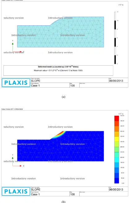
Figure 19 PLAXIS Case 1 - Simple Homogeneous Soil Slope (a)
Deformation, and (b) Total Displacement 35
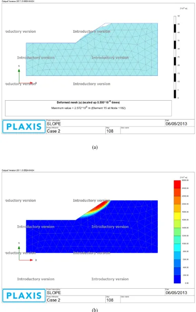
Figure 20 PLAXIS Case 2 - Simple Homogeneous Soil Slope (a)
Deformation, and (b) Total Displacement 36
Figure 21 PLAXIS Case 3 - Simple Homogeneous Soil Slope (a)
Deformation, and (b) Total Displacement 37
Figure 22 Simple Reservoir Embankment with a Clayey Soil 39 Figure 23 Image of a Reservoir Embankment (VirginiaTech 2007). 40 Figure 24 FLAC/Slope: Slope Parameters for all Cases - Simple
Reservoir Embankment 41
Figure 25 FLAC/Slope: Material Properties for Case 1 - Simple
Reservoir Embankment 42
Figure 26 FLAC/Slope Finite Element Mesh - Simple Reservoir
Embankment 42
Figure 27 FLAC/Slope Critical Slip Surface for Case 1 - Simple
Reservoir Embankment 43
Figure 28 FLAC/Slope Critical Slip Surface for Case 2 - Simple
Reservoir Embankment 44
Figure 29 FLAC/Slope Critical Slip Surface for Case 3 - Simple
Reservoir Embankment 44
Figure 30 SLOPE/W Material Properties for case 1 - Simple Reservoir
Embankment 46
Figure 31 SLOPE/W Critical Slip Surface for Case 1 - Simple Reservoir
Embankment 46
Figure 32 SLOPE/W Critical Slip Surface for Case 2 - Simple Reservoir
Embankment 47
Figure 33 SLOPE/W Critical Slip Surface for Case 3 - Simple Reservoir
Embankment 47
Figure 34 PLAXIS Finite Element Mesh - Simple Reservoir
Embankment 49
Figure 35 PLAXIS Case 1 - Simple Reservoir Embankment (a)
Figure 36 PLAXIS Case 2 - Simple Reservoir Embankment (a)
Deformation, and (b) Total Displacement 51
Figure 37 PLAXIS Case 3 - Simple Reservoir Embankment (a)
Deformation, and (b) Total Displacement 52
Figure 38 Earth Dam before Rapid Drawdown. 54
Figure 39 Earth Dam after Rapid Drawdown. 54
Figure 40 Image of an Earth Dam (U.S. Army Corps of Engineers 2013). 55 Figure 41 FLAC/Slope Slope Parameters for all Cases – Earth Dam 57 Figure 42 FLAC/Slope Material Properties – Earth Dam 57 Figure 43 FLAC/Slope Finite Element Mesh for Case 1 – Earth Dam 58 Figure 44 FLAC/Slope Critical Slip Surface before Drawdown – Earth
Dam 58
Figure 45 FLAC/Slope Critical Slip Surface after drawdown – Earth
Dam 59
Figure 46 SLOPE/W Material Properties – Earth Dam 60
Figure 47 SLOPE/W Critical Slip Surface before drawdown – Earth Dam 61 Figure 48 SLOPE/W Critical Slip Surface after drawdown – Earth Dam 61
Figure 49 PLAXIS Finite Element Mesh - Earth Dam 63
Figure 50 PLAXIS - Earth Dam before drawdown (a) Deformation, and
(b) Total Displacement 64
Figure 51 PLAXIS - Earth Dam after drawdown (a) Deformation, and (b)
Total Displacement 65
Figure 52 Results Comparison - Simple Homogeneous Soil Slope 68 Figure 53 Results Comparison - Simple Reservoir Embankment 70
Figure 54 FLAC/Slope allowed models. 72
Figure 55 FLAC coarse mesh of an Open Cut Mine Pit Wall. 74 Figure 56 SLOPE/W Critical Slip Surface before drawdown (incorrect
direction) – Earth Dam 76
List of Tables
Table 1 SLOPE/W Mohr-Coulomb Model Properties 16
Table 2 FLAC Mohr-Coulomb Model Basic Properties 20
Table 3 FLAC Mohr-Coulomb Model Advanced Properties 20
Table 4 PLAXIS Mohr-Coulomb Model Properties 22
Table 5 Unsaturated Sand Material Properties - Simple Homogeneous Soil
Slope 25
Table 6 Cases and corresponding Embankment Heights - Simple
Homogeneous Soil Slope 25
Table 7 Parameters for Analysis 26
Table 8 FLAC/Slope FOS Results - Simple Homogeneous Soil Slope 30 Table 9 SLOPE/W FOS Results - Simple Homogeneous Soil Slope 33 Table 10 PLAXIS Finite Element Modelling Construction Stages 34 Table 11 PLAXIS FOS Results - Simple Homogeneous Soil Slope 38 Table 12 Summary of FOS Results - Simple Homogeneous Soil Slope 38 Table 13 Clayey Soil Material Properties - Simple Reservoir Embankment 40 Table 14 FLAC/Slope FOS Results - Simple Reservoir Embankment 45 Table 15 SLOPE/W FOS Results - Simple Reservoir Embankment 48 Table 16 PLAXIS Finite Element Modelling Construction Stages 49 Table 17 PLAXIS FOS Results - Simple Reservoir Embankment 53 Table 18 Summary of FOS Results - Simple Reservoir Embankment 53 Table 19 Clayey Soil Material Properties - Simple Reservoir Embankment 55
Table 20 FLAC/Slope FOS Results – Earth Dam 59
Table 21 SLOPE/W FOS Results – Earth Dam 62
Table 22 PLAXIS Finite Element Modelling Construction Stages 63
Table 23 PLAXIS FOS Results – Earth Dam 66
Table 24 Summary of FOS Results – Earth Dam 66
Table 25 FOS Differences (%) - Simple Homogeneous Soil Slope 67 Table 26 FOS Differences (%) - Simple Reservoir Embankment 69 Table 27 FOS Differences (%) before Rapid Drawdown – Earth Dam 71 Table 28 FOS Differences (%) after Rapid Drawdown – Earth Dam 71
Nomenclature
FOS Factor of safety
LE Limit Equilibrium
FE Finite Element
FD Finite Difference
SRF Strength Reduction Factor
Z Depth
s Shear strength
τ Shear stress
σ Normal stress
σ' Effective normal stress
ρ Density
unsat Unsaturated unit weight
sat Saturated unit weight
u Pore water pressure
c' Drained cohesion
'
Drained friction angle
c Undrained cohesion
Undrained friction angle
E’ Drained Elastic (Young’s) modulus
E Undrained Elastic (Young’s) modulus
Chapter 1: Introduction
1.1
Introduction
The purpose of this report is to compare the student versions of FLAC, PLAXIS and SLOPE/W and their use in Geotechnical stability analysis.
The instability of a slope is an ongoing concern in most construction and infrastructure projects, as slope failures can result in significant repair and maintenance costs and can endanger both the workers and the general public. There are a number of software packages that have been developed for geotechnical stability analysis which utilise the Limit Equilibrium (LE) Method, Finite Element (FE) method and Finite Difference (FD) method. The LE method is the most widely used approach; however it does contain several limitations and inconsistencies. With the advancement in technology software packages utilising the FE and FD methods have increased in popularity as they tend to possess a wider range of features (Hammouri et al. 2008).
This research project intends to compares three software packages and their respective methods of stability analysis.
LE method:
SLOPE/W is a software package created by GEO-SLOPE International Ltd. as part of their GeoStudio bundle.
FE/FD methods:
PLAXIS is a software package created by Plaxis bv..
1.2
Background
Over the years there has been an increase in construction and infrastructure projects and consequently a growth in the requirements for excavation, footings and road design. Engineers must take into account all geotechnical aspects affecting their design including soil material properties, slope stability and possible natural disasters which can have devastating social and economic impacts. Incorporating the analysis of slope stability within the design will help in the prevention of any geotechnical failures throughout construction and the life of the design (Bromhead 1992).
Slope stability is important throughout all aspects of construction and a small difference in the calculated Factor of Safety (FOS) can result in a significant increase in costs both in construction and ongoing maintenance. For many years the LE method has been the most common approach due to its simplicity and requiring minimal properties; however with the advancement in technology there has been an increase in the use of the FE and FD methods; as they are able to accommodate a wider range of geometries and can progressively calculate the deformation and stresses on the model up to and including the FOS. Currently there is no evidence into which software packages produce the most acceptable results. This research project intends to assist the engineering industry in comparing the student versions of SLOPE/W, PLAXIS & FLAC; three packages widely used (Aryal 2008).
1.3
Methodology
The methodology employed in addressing this report involves:
i) Studying the background into the methodology of the 3 software packages; PLAXIS, FLAC & SLOPE/W. i.e. Finite Element Method, Finite Difference Method & Limit Equilibrium Method.
iv) Research scenarios of geotechnical stability in which the software packages can be used.
v) Create concepts for each scenario to analyse.
vi) Research each scenario’s parameters and soil properties.
vii) Create detailed scenarios including the geometry, details or actions and soil properties.
viii) Analyse each scenario using FLAC, PLAXIS & SLOPE/W and discuss the results.
ix) From all the above steps discuss the limitations and benefits of each of the software packages and make recommendations.
1.4
Objectives
The objectives of this report include:
Gain a better understanding of factors that cause slope instability and their importance in the geotechnical analysis.
Gain a better understanding of the student versions of FLAC, PLAXIS and SLOPE/W.
Discuss the benefits and limitations of each packages student version. Evaluate my own personal experiences and preferences in the packages.
1.5
Report Structure
Chapter 1: Introduction Outlines the problem explored within the report.
Chapter 2: Literature Review Reviews the current literature
that has been published.
Chapter 3: Software Packages Outlines the software
packages used for the report.
Chapter 4: Scenario 1 - Simple Homogeneous
Soil Slope at Varying Heights.
Outlines the scenario and results.
Chapter 5: Scenario 2 - Simple reservoir
embankment with a clayey soil of varying
plasticity.
Outlines the scenario and results.
Chapter 6: Scenario 3 - Earth Dam suffering
rapid drawdown.
Outlines the scenario and results.
Chapter 7: Results and Discussion Analysis of the results and
discussion of the software used.
Chapter 8: Conclusion Conclusion and
Chapter 2: Literature Review
2.1 Introduction
This chapter serves to review the current literature that has been published regarding FLAC, PLAXIS and SLOPE/W and their corresponding stability analysis methods. The majority of published information is in regards to the analysis methods of Limit Equilibrium, Finite Element and Finite Difference and not the software packages themselves. This literature review intends to establish an understanding of each of these methods.
2.2 Limit Equilibrium (LE) Method
Currently the LE method is the most widely used approach within the geotechnical industry in solving modern day slope stability scenarios. The LE method requires the plastic Mohr-Coulomb criterion where a materials failure is due not from the maximum normal or shear stress alone but a combination of both. The LE method establishes the required soil properties; slope geometry and then using the Mohr-Coulomb criterion calculates the stability of the slope by comparing the forces causing failure against the resisting forces. Throughout this procedure an FOS is computed using the equations of static equilibrium. “The fundamental assumption…is that failure occurs through sliding of a block or mass along a slip surface” (RocScience 2004a, p.2) and in order to compute the appropriate FOS a number of slip surfaces need to be postulated to find the
critical slip surface. (Duncan & Wright 2005; Hammouri et al. 2008; Chen & Liu 1990, Das 2010).
The LE method requires the following assumptions:
i) “The soil behaves as a Mohr-Coulomb material.
iii) Each block within the slip surface has the same FOS.
iv) Inter-slice forces are assumed; to deem the problem determinate (Griffiths & Lane 1999; Cheng & Lau 2008; Aryal 2008).
2.2.1 Vertical Slices
The LE method utilises the method of vertical slices, the vertical slices method is where “the entire sliding mass is divided into a reasonable number of slices and the inter-slice forces are computed based on an assumed inter-slice force functional relationship” (Aryal 2008, p.4509). Slip surfaces are assumed and the static equilibrium equations are used to calculate the stresses and FOS on each slice (Chen & Lau 2008).
The static equilibrium conditions are:
1. “Equilibrium of forces in the vertical direction, 2. Equilibrium of forces in the horizontal direction, and
3. Equilibrium of moments about any point” (Duncan & Wright 2005, p.56).
The slip surface is a surface where sliding is assumed to occur; this slip surface may be circular, or a shape defined by straight lines. Duncan and Wright, 2005 states that when using the LE method the Morgenstern-Price procedure should be adopted as it satisfies all requirements for static equilibrium requirements for both forces and moments. The Morgenstern-Price procedure creates ‘blocks’
dividing the soil above the slip surface.
Figure 1 Static Scheme – Morgenstern-Price Method (Fine-Civil Software Package 2013).
The following assumptions are introduced in the Morgenstern-Price method to calculate the limit equilibrium of forces and moment on individual blocks:
dividing planes between blocks are always vertical;
the line of action of weight of block Wi passes through the center of the ith segment of slip surface represented by point M;
the normal force Ni is acting in the center of the ith segment of slip surface, at point M;
inclination of forces Ei acting between blocks is different on each block (δi) at slip surface end points is δ = 0.” (Fine-Civil Software Package, 2013)
2.2.2 Benefits
The LE method has the following benefits:
It is a simplistic approach.
Requires minimal soil properties and slope geometry.
An adequate design based upon the calculated FOS ensures that sliding along the slip surface should not occur.
2.2.3 Limitations
The LE method has several limitations, including:
Numerical inconsistencies.
The analysis method is the same for all scenarios; i.e. the same method is used for a “slope of a newly constructed embankment, a slope of a recent excavation, or an existing natural slope” (Zheng et.al. 2008, p.629).
Neglects the stress-strain behaviour of the material.
The user needs an understanding of the geotechnical and slope stability principals involved within the analysis i.e. the direction of the slip surface. Unable to model the progressive failure and deformation of the surface
without assumptions being made. (Cheng & Lau 2008; Hammouri et al. 2008; RocScience 2004a).
2.2.4 Factor of Safety (FOS)
The FOS is considered the magnitude the soils ultimate shear strength must be reduced by in order for failure to occur (Cheng & Lau 2008; Zheng et.al. 2008; Griffiths & Lane 1999; GEO-SLOPE International 2004).
According to Duncan & Wright (2005), the most extensively used definition of FOS for slope stability is:
Using the Mohr-Coulomb equations, the shear strength can be expressed in terms of total stresses or effective stresses.
Total stress analysis:
Effective stress analysis:
Cheng & Lau (2008) states the LE method assumes the FOS to be constant along a slip surface and can be defined with respect to either the force or moment equilibrium:
1. Moment Equilibrium: used for rotational analysis (i.e. landslides).
Where;
FOSm = factor of safety defined with respect to moment
Md = summation of the driving moment
2. Force equilibrium: applies to translational or rotational failure (i.e. planar slip surfaces).
Where;
FOSf = factor of safety defined with respect to force
Fr = summation of the resisting forces
Fd = summation of the driving forces
2.3 Finite Element (FE) Method
“The FE method is a numerical technique for solving differential equations or boundary value problems in science and engineering” (Hammouri et al. 2008, p.472). The FE method has been adapted for geotechnical engineering; however there is a perception by professionals in the geotechnical industry that the FE method is too complex and there is criticism in its necessity compared to the simpler LE method considering the poor quality of materials properties often used in the analysis (Griffiths & Lane 1999).
2.3.1 Finite Difference (FD) Technique
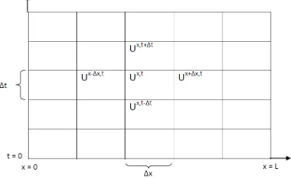
[image:26.595.124.540.350.605.2]With regards to geotechnical engineering it can be considered that the Finite Difference (FD) technique is a special case of the FE approach. Both methods involve differential equations being transformed into matrix equations for each element; even though the equations are derived using two different methods the resulting equations are identical. The FD technique involves replacing the given continuous derivative terms with an “algebraic express written in terms of field variables (e.g. stress or displacement) at discrete points in space” (Itasca Consulting Group 2011a, p.1). These newly formed equations relate unknown dependent variables to given initial values and/or boundary conditions. There are 3 different possible techniques. Below is an example of all three (Wikipedia 2013; Itasca Consulting Group 2011a; Stephenson & Meados 1986).
Figure 2 Rectangular mesh showing nodal points used in the finite difference technique.
Backward difference in x-direction
Central difference in x-direction
Once the differential equations have been manipulated so they rely on known nodal points it can be seen from the above three examples that it is relatively easy to find the corresponding unknown values. This is an example using a simplistic rectangular mesh however this technique can be used for any shaped mesh.
For the FE and FD approach the element matrices for an elastic material are identical (Itasca Consulting Group 2011a).
2.3.2 Benefits
With the advancement of technology there has been a large increase in the use of the FE and FD methods specifically in slope stability analysis. The FE and FD methods have the following benefits:
The analysis can run relatively quickly.
The FD method is a simple approach.Able to monitor progressive failure of the soil up to and including the FOS.
Can accommodate a wide range of slope geometries and problems.
The failure occurs within the slope where the resisting forces are outweighed by the driving forces. That is no assumptions are required regarding the location and direction of the slip surface models.
Is able to calculate deformation, stresses and pore pressures within the slope (Desai & Christian 1977; Griffiths & Lane 1999; Hammouri et al. 2008).
2.3.3 Limitations
Although many believe the FE and FD methods overcome the LE method’s deficiencies, it has its limitations, including:
Calculated FOS can be dependent of the relative conditions chosen An inexperienced user may not be aware of meshing errors, boundary
conditions or time restrictions involved in the analyses.
The FD technique can run analysis slower than the FE method, particularly for linear problems.
The FE and FD method are considered more complex compared to the LE method. Within the industry this complexity can be considered unnecessary – due to the relative inaccuracy of field data. (Zheng et.al. 2008; Griffiths & Lane 1999; Itasca Consulting Group 2011a; Wikipedia 2013).
2.3.4 Factor of Safety (FOS)
To determine the FOS the shear strength reduction technique is incorporated and extends off the FE and FD methods. “The factored shear strength parameters c’f
and Ф’fare therefore given by:
A systematic iterative approach is undertaken to determine the SRF that applies to both terms. The ‘true’ FOS is equal to the SRF at the first instance of failure. That is FOS = SRF (Griffiths & Lane 1999).
Chapter 3: Software Packages
3.1 Overview
This research project compares three of the more predominant software packages used within the Geotechnical Engineering industry for slope stability analyses. Due to licensing requirements of each software package this project compares the student (demonstration) version of each package.
The software packages and their respective methods of stability analysis are:
LE method:
GEO-SLOPE International Ltd, SLOPE/W 2012 Version 8.0 – Student License.
o Operating system Microsoft Windows 7.
FE/FD methods:
ITASCA Consulting Group Inc, FLAC 2011 Version 7.0 – Demonstration Mode.
o Operating system Microsoft Windows 7.
Plaxis bv., PLAXIS Version 2010 – Introductory Version.
o Operating system Microsoft Windows 7.
3.2 SLOPE/W
3.2.1 Required Soil Properties
SLOPE/W requires soil properties that satisfy the Mohr-Coulomb Criterion. The properties required to produce a valid soil model are presented in Table 1.
Property Symbol Units Definition
Unit Weight γ kN/m3 Soil’s Total Unit Weight
Cohesion c kPa Soil’s Cohesion
Phi ˚ Soil’s Friction Angle
Table 1 SLOPE/W Mohr-Coulomb Model Properties
3.2.2 Slip Surface Entry & Exit
The Entry and Exit command allows the user to identify slip surfaces by specifying the assumed portion of the surface where the slip surface will enter and exit. (GEO-SLOPE International 2012).
“The entry and exit ranges are used to determine a group of circular trial slip surfaces.” (GEO-SLOPE International 2012). The slip surface with the smallest FOS is taken as the critical slip surface. This method is considered more intuitive than the ‘Grid & Radius’ approach; however consideration must be made for the direction of the slip surface and if the critical slip surface extends beyond the entry and exit range specified (GEO-SLOPE International 2012).
3.2.3 SOLVE Process
SLOPE/W uses the SOLVE process to calculate the FOS. Each slip surface is processed in 3 steps:
1. Initially no forces are considered between the slices.
3. Then normal and shear force relationship is considered. In the case of the
Morgenstern-Price method, where the moment and force FOS are calculated within a specified convergence (GEO-SLOPE International 2004).
3.2.4 Morgenstern-Price Method
Cheng (2008) states that the different methods derived for LE (such as
Morgenstern-Price, Spencer, Janbu, etc) should achieve similar FOS results. However, the Morgenstern-Price method is considered the most popular approach as it satisfies both force and moment equilibrium and applies to almost all soil profiles and slope geometries. The method involves dividing the sliding mass into vertical slices, which requires assumptions regarding the inter-slice shear forces (Zhu et al. 2005; GEO-SLOPE International 2004; Duncan & Wright 2005; Bromhead 1992).
Figure 4 presents the plot of FOS against lambda (λ) for various methods. The relationship between shear and normal inter-slice forces is represented by λ and the two curves illustrate the FOS with respect to moment equilibrium compared to the FOS with respect to force equilibrium. It can be seen that there is a variation in FOS for a range of λ values (GEO-SLOPE International 2004).
Figure 4 Moment and Force FOS as a Function of the Inter-slice Shear Force (GEO-SLOPE International 2004)
3.3 FLAC
“FLAC is a two-dimensional explicit finite difference program for engineering mechanics computation. This program simulates the behaviour of a structure built of soil, rock, or other materials that may undergo plastic flow when their yields limits are reached” (ITASCA Consulting Group 2011a, p.1). FLAC finds the static solutions for a problem using the two-dimensional plane-strain model. However, the dynamic equations of motion are included in the formulation to help model the stable and unstable forces within the model; this ensures that the scenario of a sudden collapse within the model is accounted for.
the velocities and displacements; then the new stresses and strain rates are calculated and so forth until failure is achieved. Note that a relatively small time step is chosen to ensure that the stress changes of each element do not influence its neighbours (ITASCA Consulting Group 2011b).
3.3.1 Required Soil Properties
FLAC requires basic soil parameters to simulate the shear strength characteristic of a soil. In addition to the basic parameters, advanced properties may be provided when using the Mohr-Coulomb model. The properties required for the Mohr-Coulomb model used in this analysis are outlined in Table 2and Table 3.
Property Symbol Units Definition
Density p kg/m3 Density of the soil
Cohesion c Pa The cohesion component of the shear strength
Phi ˚ Friction angle of the soil
Table 2 FLAC Mohr-Coulomb Model Basic Properties
Property Symbol Units Definition
Tension t Pa The tensile component of the shear strength
Psi Ψ ˚ Dilation angle of the soil
Table 3 FLAC Mohr-Coulomb Model Advanced Properties
Note that for a basic Mohr-Coulomb model it is assumed that the dilation angle is equal to the friction angle (Ф = Ψ) and the tensile strength is high enough to prevent tension cut-off. (ITASCA Consulting Group 2011a)
3.3.2 FLAC/Slope
“FLAC/Slope is a mini-version of FLAC that is designed specifically to perform factor-of-safety calculations for slope stability.” (ITASCA Consulting Group 2011b, p.1).
FLAC/Slope allows for quick analysis of relatively basic scenarios, with certain model templates already loaded and properties of certain materials pre-loaded. The FLAC/Slope manual states that the FD method is a practical alternative to the LE method software packages and provides the following benefits:
2. No artificial parameters (e.g., functions for interslice force angles) need to be given as input.
3. Multiple failure surfaces (or complex internal yielding) evolve naturally, if the conditions give rise to them.
4. Structural interaction (e.g., rockbolt, soil nail or geogrid) is modelled realistically as fully coupled deforming elements, not simply as equivalent forces.
5. The solution consists of mechanisms that are kinematically feasible. (Note that the limit equilibrium method only considers forces, not kinematics.)” (ITASCA Consulting Group 2011b, p.1).
In addition to the FOS being calculated; FLAC/Slope creates a plot indicating the shear-strain rate of the elements which outline the failure surface and indicates the failure mode.
FLAC/Slope will be used for all analysis of the FLAC component within this report.
3.4 PLAXIS
PLAXIS is described as a FE package for geotechnical analysis that can utilise both two-dimensional and three-dimensional analysis in determining the stability and deformation experienced by slopes. PLAXIS lends itself to modeling more complex geotechnical scenarios as it has the capabilities to simulate inhomogeneous soil properties and time-dependent scenarios (Brinkgreve 2002; Hammouri et al. 2008; Plaxis bv. 2012a).
appropriately judgement on the reliability of the results obtained (Plaxis bv. 2012c).
3.4.1 Required Soil Properties
In addition to the basic Mohr-Coulomb parameters, several advanced properties may be utilised. These properties are outlined in Table 4.
Property Symbol Units Definition
Saturated Unit
Weight γsat kN/m
3 Unit weight of soil below phreatic level
Unsaturated Unit
Weight γunsat kN/m
3 Unit weight of soil above phreatic level
Phi ˚ Friction angle of the soil
Poisson’s Ratio ν - The ratio of lateral strain to linear
strain
Reference Elastic
Modulus Eref kN/m
2
Elastic modulus at the reference depth
Reference
Cohesion cref kN/m
2
Cohesion at the reference depth
Table 4 PLAXIS Mohr-Coulomb Model Properties
3.4.2 Elastic Modulus (E)
3.4.3 Staged Construction
The staged construction approach intends to simulate the various stages throughout the slopes construction. This involves activating and/or deactivating the appropriate loads, geogrids, interfaces or soil layers throughout the analysis. The benefit of this approach is that it has the ability to take time into account (Plaxis bv. 2012b).
3.4.4 Phi-c Reduction
Chapter 4: Scenario 1 – Simple Homogeneous Soil
Slope at Varying Heights
4.1 Geotechnical Model
The geotechnical model adopted in this analysis is illustrated in Figure 6. The soil is classified as unsaturated sand and comprises of the properties in Table 5, kept constant throughout all analyses.
The slope considered has an embankment batter of 1:1.5, producing a slope angle equal to 33.7˚. The embankment height varies from 4m to 8m, with each case increasing in 2m increments, totalling 3 cases. No water table has been considered.
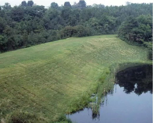
Figure 7 Image of a Road Embankment (Terracon 2013) Figure 6Simple Homogeneous Soil Slope
Unsaturated Sand Varies
1.5
1
10m
4.1.1 Material Properties
The properties of the unsaturated sand material are presented in Table 5. These properties are adequate for the Mohr-Coulomb approach. The embankment will be analysed for 3 cases at varying heights, presented in Table 6.
Material
Unit Weight (kN/m3)
Elastic Modulus (MPa) Poisson’s Ratio Cohesion (kPa) Friction Angle (˚) Unsaturated
Sand 17 13 0.3 1 30
Table 5 Unsaturated Sand Material Properties - Simple Homogeneous Soil Slope
Case Embankment Height (m)
Case 1 4
Case 2 6
Case 3 8
Table 6 Cases and corresponding Embankment Heights - Simple Homogeneous Soil Slope
4.1.2 Units
Property Symbol Units PLAXIS & SLOPE/W Units FLAC/Slope
Unit Weight / Density γ / p kN/m3 kg/m3
Cohesion c kPa Pa
Friction angle ˚ ˚
Elastic Modulus E MPa = 103 kN/m2 -
Poisson’s Ratio ν - -
Table 7 Parameters for Analysis
4.2 FLAC/Slope Analysis
4.2.1 Methodology
i) Upon starting FLAC/Slope a model name and embankment form needs to be chosen. This model is a simple embankment.
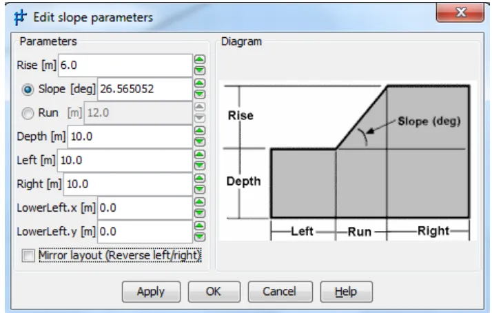
ii) The slope parameters need to be entered. The slope parameters for Case 1 are presented in Figure 8.
iii) The material properties need to be created and assigned. It must be noted that FLAC requires the Density of the material and the Cohesion inputted in Pascals as presented in Figure 9. The material is then assigned to the embankment. Note that a standard porosity of 0.5 is assigned but is not relevant as there is no water table.
iv) A mesh needs to be assigned to the embankment. Due to the limitations of the student package of FLAC/Slope a coarse mesh is used, presented in Figure 10. This may affect the accuracy of the results.
Figure 8 FLAC/Slope Slope Parameters for Case 1 - Simple Homogeneous Soil Slope
4.2.2 Results
[image:43.595.117.551.48.267.2]Figure 11 to Figure 13 illustrate the critical slip surfaces for Cases 1 to 3 respectively using FLAC/Slope. Table 8 summarises the FOS results using FLAC/Slope. Note that due to the restrictions of a coarse mesh the contour plot is not very accurate.
Figure 10 FLAC/Slope Finite Element Mesh for Case 1 - Simple Homogeneous Soil Slope
Figure 12 FLAC/Slope Critical Slip Surface for Case 2 - Simple Homogeneous Soil Slope
Table 8 outlines the FOS results from the FLAC/Slope analysis using a coarse mesh.
Table 8 FLAC/Slope FOS Results - Simple Homogeneous Soil Slope
4.3 SLOPE/W Analysis
4.3.1 Methodology
i) Upon starting SLOPE/W the first step is to set the units and scale for the model, then axes can be drawn.
ii) The model is drawn using the inbuilt CAD interface. Alternatively a model drawing can be imported from such programs as AutoCAD. As this is a simple slope with one region sketching the model with the region function is relatively simple. For models with multiple regions and materials using the Sketch polylines function then applying the region function of the appropriate areas can be more functional.
iii) The material properties need to be created and assigned, presented in Figure 14. The material is then assigned to the embankment.
iv) The slip surface is selected, and then the model can be solved.
v) This process is done for each case. Figure 15 to Figure 17 illustrate the critical slip surfaces for the 3 cases.
Case FOS
Case 1 1.38
Case 2 1.18
4.3.2 Results
Figure 15 to Figure 17 illustrate the critical slip surfaces for Cases 1 to 3 respectively using SLOPE/W. Table 9 summarises the FOS results using SLOPE/W.
Figure 14 SLOPE/W Material Properties - Simple Homogeneous Soil Slope
Figure 16 SLOPE/W Critical Slip Surface for Case 2 - Simple Homogeneous Soil Slope
Table 9 SLOPE/W FOS Results - Simple Homogeneous Soil Slope
4.4 PLAXIS Analysis
4.4.1 Methodology
i) Upon starting PLAXIS the projects title and models units and dimensions need to be set.
ii) The model is drawn using the inbuilt CAD interface.
iii) The material properties need to be created and assigned. PLAXIS requires the advanced properties of E and ν of the soil as well as the standard Mohr-Coulomb.
iv) The restraints are then set as standard fixities.
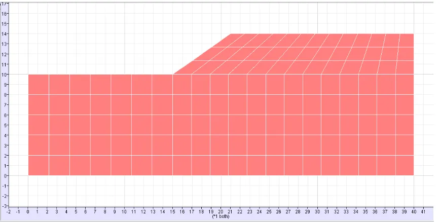
v) The mesh is generated. A medium mesh is being used to help improve accuracy. The mesh for Case 1 is presented in Figure 18.
vi) In the calculation phase, the stability of the embankment needs to be simulated, Table 10 summarises each phase modelled in the PLAXIS assessment.
vii) The results are then viewed showing deformation, total displacement, FOS etc.
viii) This process is done for each case. Figure 19 to Figure 21 illustrate the critical slip surfaces for the 3 cases.
Case FOS
Case 1 1.185
Case 2 1.122
Table 10 PLAXIS Finite Element Modelling Construction Stages
4.4.2 Results
Figure 19 to Figure 21 illustrate the critical slip surfaces for Cases 1 to 3 respectively using PLAXIS. Table 11 summarises the FOS results using PLAXIS.
Phase Description Analysis
Type Loading Input
Time Period (day)
0 Set up initial
ground model Initial - -
1 Embankment
Construction Plastic
Staged
Construction 1
2 FOS Analysis Phi-c
Reduction
Incremental
Multipliers -
(a)
(b)
[image:50.595.108.528.60.716.2](a)
[image:51.595.122.517.91.720.2](b)
(a)
(b)
Table 11 outlines the FOS results from the PLAXIS analysis.
Table 11 PLAXIS FOS Results - Simple Homogeneous Soil Slope
4.5 Summary of Simple Homogeneous Soil Slope Results
The slope stability analysis has been conducted using FLAC/Slope, SLOPE/W and PLAXIS. Table 12 outlines the calculated FOS values from the proposed analysis methods. It can be seen that the SLOPE/W and PLAXIS analysis produce similar results; however the FLAC/Slope analysis results are significantly different. This is due to the coarse mesh used in the FLAC/Slope analysis producing results that can be considered not as accurate as the SLOPE/W and PLAXIS analysis.
Analysis Method FOS
Case 1 Case 2 Case 3
FLAC/Slope 1.38 1.18 1.10
SLOPE/W 1.185 1.122 1.064
PLAXIS 1.208 1.100 1.057
Table 12 Summary of FOS Results - Simple Homogeneous Soil Slope
Case FOS
Case 1 1.208
Case 2 1.100
Chapter 5: Scenario 2 – Simple Reservoir
Embankment with a Clayey Soil of Varying
Plasticity
5.1 Geotechnical Model
The geotechnical model adopted in this analysis is illustrated in Figure 22. The soil is classified a clayey soil with varying plasticity comprising of the properties in Table 13.
The slope considered has an embankment batter of 1:2, producing a slope angle equal to 26.6˚. The reservoir height is kept constant at 6m, with the water table for each case at 4m.
Figure 22 Simple Reservoir Embankment with a Clayey Soil
Clayey Soil
4m
2
1
10m
Figure 23 Image of a Reservoir Embankment (VirginiaTech 2007).
5.1.1 Material Properties
The properties of the clayey soil are presented in Table 13. All properties are kept constant except the friction angle. These properties are adequate for the Mohr-Coulomb approach.
Material Cases
Unsaturated Unit Weight
(kN/m3)
Saturated Unit Weight (kN/m3)
Elastic Modulus (MPa) Poisson’s Ratio Cohesion (kPa) Friction Angle (˚) Clayey Soil
Case 1 16 18 3 0.15 6 24
Case 2 16 18 3 0.15 6 20
[image:55.595.192.454.42.251.2]Case 3 16 18 3 0.15 6 17
Table 13Clayey Soil Material Properties - Simple Reservoir Embankment
5.1.2 Units
5.2
FLAC/Slope Analysis
5.2.1 Methodology
i) Upon starting FLAC/Slope a model name and embankment form needs to be chosen. This model is a simple embankment.
ii) The slope parameters then need to be entered. The slope parameters are kept constant for all 3 cases, presented in Figure 24.
iii) The material properties need to be created and assigned similar to Scenario 1. All properties are kept constant for each case except the friction angle; the properties for Case 1 are presented in Figure 25. The material is then assigned to the reservoir
iv) The water table is assigned 4 meter above ground i.e. 14 meters. v) A mesh is assigned to the reservoir. Due to the limitations of the
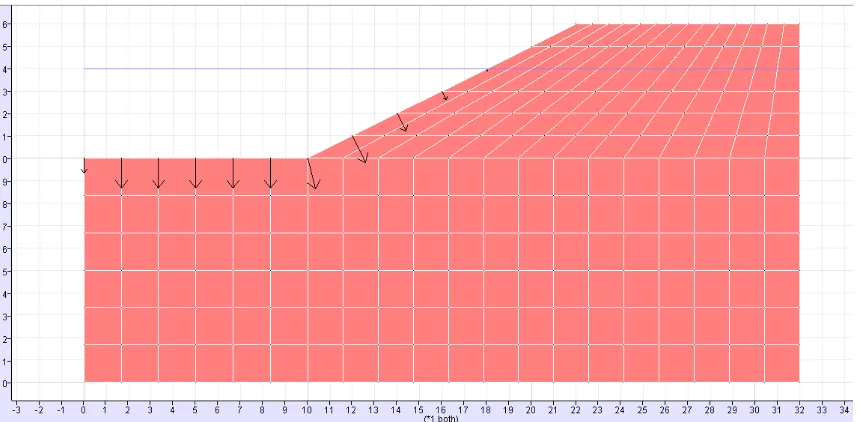
student version of FLAC/Slope (limit on the amount of zones that can be analysed) a coarse mesh is used, presented in Figure 26. This may affect the accuracy of the results.
[image:56.595.163.520.502.729.2]vi) The embankment is cloned and each Case’s friction angle updated. Each case is solved giving an estimate for the FOS and a plot of the corresponding critical slip surfaces. Figure 27 to Figure 29 illustrate these critical slip surfaces.
Figure 25 FLAC/Slope: Material Properties for Case 1 - Simple Reservoir Embankment
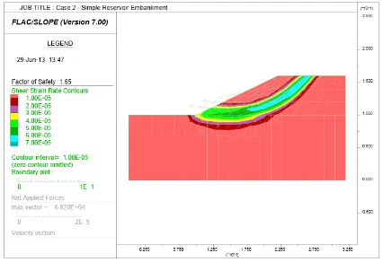
[image:57.595.117.548.448.659.2]5.2.2 Results
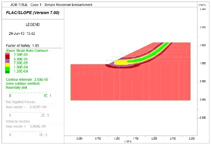
[image:58.595.114.537.233.524.2]Figure 27 to Figure 29 illustrate the critical slip surfaces for Cases 1 to 3 respectively using FLAC/Slope. Table 14 summarises the FOS results using FLAC/Slope. Note that due to the restrictions of a coarse mesh the shear-strain contour plot is not very accurate.
Figure 28 FLAC/Slope Critical Slip Surface for Case 2 - Simple Reservoir Embankment
Table 14 outlines the FOS results from the FLAC/Slope analysis using a coarse mesh. Note if a medium/fine mesh is chosen an error occurs as they create more zones than allowed in the student version.
Table 14 FLAC/Slope FOS Results - Simple Reservoir Embankment
5.3
SLOPE/W Analysis
5.3.1 Methodology
i) Upon starting SLOPE/W the first step is to set the units and scale for the model, then axes can be drawn.
ii) The model must be drawn using the inbuilt CAD interface. As this is a simple slope with one region the model can be sketched with the region function.
iii) The material properties need to be created and assigned. Figure 30 presents the material properties for Case 1. The material is then assigned to the reservoir.
iv) The water table is drawn in using the Pore-Water Pressure function. v) The slip surface must then be selected, and the model can be solved. vi) This process is done for each case. Figure 31 to Figure 33 illustrate the
critical slip surfaces for the 3 cases.
Case FOS
Case 1 1.85
Case 2 1.65
5.3.2 Results
[image:61.595.154.486.71.308.2]Figure 31 to Figure 33 illustrate the critical slip surfaces for Cases 1 to 3 respectively using SLOPE/W. Table 15 summarises the FOS results using SLOPE/W.
[image:61.595.116.546.470.736.2]Figure 30 SLOPE/W Material Properties for case 1 - Simple Reservoir Embankment Figure 9 SLOPE/W Critical Slip Surface for Case 1 - Simple Homogeneous Soil Slope
Figure 32 SLOPE/W Critical Slip Surface for Case 2 - Simple Reservoir Embankment
Table 15 outlines the FOS results from the SLOPE/W analysis.
Table 15 SLOPE/W FOS Results - Simple Reservoir Embankment
5.4
PLAXIS Analysis
5.4.1 Methodology
i) Upon starting PLAXIS the projects title and the models units and dimensions need to be set.
ii) The model is drawn using the inbuilt CAD interface.
iii) The material properties need to be created and assigned. PLAXIS requires the advanced properties of E and ν of the soil as well as the stand Mohr-Coulomb.
iv) The restraints are set as standard fixities.
v) Then the mesh is generated. A medium mesh is being used to help improve accuracy. The mesh is presented in Figure 34.
vi) In the calculation phase, the stability of the reservoir and the water table need to be simulated, Table 16 summarises each phase modelled in the PLAXIS assessment.
vii) The results are then viewed showing the deformation, total displacement, FOS etc.
viii) This process is done for each case. Figure 35 to Figure 37 illustrate the critical slip surfaces for the 3 cases.
Case FOS
Case 1 1.812
Case 2 1.629
Table 16 PLAXIS Finite Element Modelling Construction Stages
3.4.2 Results
Figure 35 to Figure 37 illustrate the critical slip surfaces for Cases 1 to 3 respectively using PLAXIS. Table 17 summarises the FOS results using PLAXIS.
Phase Description Analysis
Type Loading Input
Time Period
(day)
0 Set up initial
ground model Initial - -
1 Reservoir
Construction Plastic
Staged
Construction 1
2 FOS Analysis Phi-c
Reduction
Incremental
[image:64.595.116.525.335.624.2]Multipliers -
(a)
(b)
[image:65.595.114.536.98.377.2](a)
(b)
[image:66.595.117.533.69.345.2](a)
(b)
[image:67.595.117.538.70.352.2]Table 17 outlines the FOS results from the PLAXIS analysis.
Table 17 PLAXIS FOS Results - Simple Reservoir Embankment
5.5 Summary of Simple Homogeneous Soil Slope Results
The slope stability analysis has been conducted using FLAC/Slope, SLOPE/W and PLAXIS. Table 18 outlines the calculated FOS values from the proposed analysis methods. It can be seen that throughout the analysis the largest and smallest FOS values are calculated using FLAC/Slope and PLAXIS respectively. This shows that the size of the mesh used in calculations has a significant impact on the results.
Analysis Method FOS
Case 1 Case 2 Case 3
FLAC/Slope 1.85 1.65 1.49
SLOPE/W 1.812 1.629 1.481
PLAXIS 1.74 1.548 1.409
Table 18Summary of FOS Results - Simple Reservoir Embankment
Case FOS
Case 1 1.74
Case 2 1.548
Chapter 6: Scenario 3 – Earth Dam Suffering
Rapid Drawdown
6.1 Geotechnical Model
The geotechnical model adopted in this analysis is an Earth Dam suffering Rapid Drawdown, illustrated in Figure 38 and Figure 39. The soil is classified as sand and comprises of the properties in Table 19, kept constant in all analyses.
Figure 38 Earth Dam before Rapid Drawdown.
3
2
10m 10m 4m
75m
75m 10m
14m
Figure 39 Earth Dam after Rapid Drawdown.
3
The dam considered has an embankment batter of 2:3, producing a slope angle equal to 33.7˚. The dam height is kept constant at 14m, with the water table initially at 10m on the left side of the dam and ground level on the right; then drawing down to ground level on both sides.
Figure 40 Image of an Earth Dam (U.S. Army Corps of Engineers 2013).
6.1.1 Material Properties
The properties of the sand are presented in Table 19. All properties are kept constant throughout all analyses. These properties are adequate for the Mohr-Coulomb approach.
Material
Unsaturated Unit Weight
(kN/m3)
Saturated Unit Weight (kN/m3)
Elastic Modulus (MPa) Poisson’ s Ratio Cohesion (kPa) Friction Angle (˚) Unsaturated Sand
[image:70.595.184.483.174.395.2]20 26 20 0.33 5 40
6.1.2 Units
All units used are Metric, the same as in Scenario 1 and 2. Gravity is taken as 9.18m/s-2.
6.2
FLAC/Slope Analysis
6.2.1 Methodology
i) Upon starting FLAC/Slope a model name and embankment form needs to be chosen. This model is a simple dam.
ii) The slope parameters need to be entered. The slope parameters are kept constant in both cases, presented in Figure 41.
iii) The material properties need to be created and assigned similar to in Scenario 1 and 2. All properties are kept constant for both case; these properties are presented in Figure 42. The material is then assigned to the dam.
iv) For the Earth Dam before drawdown, the water table is assigned 10 meter above ground level on the left side of the embankment and ground level on the right side.
v) A mesh is assigned to the dam. Similar limitations regarding the amount of zones occurs, however for this model a medium mesh can be used, presented in Figure 43. This may affect the accuracy of the results.
Figure 41 FLAC/Slope Slope Parameters for all Cases – Earth Dam
6.2.2 Results
Figure 44 to Figure 45 illustrate the critical slip surfaces for Cases 1 to 3 respectively using FLAC/Slope. Table 20 summarises the FOS results using FLAC/Slope.
[image:73.595.118.530.446.731.2]Figure 43 FLAC/Slope Finite Element Mesh for Case 1 – Earth Dam
Table 20 outlines the FOS results from the FLAC/Slope analysis using a medium mesh. Note if a fine mesh is chosen an error occurs as they create more zones than allowed in the student package.
Table 20FLAC/Slope FOS Results – Earth Dam
6.3 SLOPE/W Analysis
6.3.1 Methodology
i) Upon starting SLOPE/W the first step is to set the units and scale for the model, then axes can be drawn.
Case FOS
Before drawdown 1.66
After drawdown 0.99
ii) The model is then drawn using the inbuilt CAD interface. As this is a simple dam with one region the model can be sketched with the region function.
iii) The material properties need to be created and assigned. Figure 46 presents the material properties. The material is assigned to the dam. iv) The water table is drawn in using the Pore-Water Pressure function. v) The slip surface is selected, and then the model can be solved. It must
be noted that the correct direction of the slip surface must be determined in order to achieve the correct factor of safety, presented in Figure 47.
[image:75.595.117.522.423.713.2]vi) The model is re analysed with the water relocated to replicate Figure 39 - after drawdown. Figure 48 presents the critical slip Note the opposite direction of the critical slip surfaces before and after drawdown.
6.3.2 Results
Figure 47 to Figure 48 illustrate the critical slip surfaces for before and after drawdown respectively using SLOPE/W. Table 21 summarises the FOS results using SLOPE/W.
Figure 47 SLOPE/W Critical Slip Surface before drawdown – Earth Dam
Table 21 outlines the FOS results from the SLOPE/W analysis.
Table 21 SLOPE/W FOS Results – Earth Dam
6.4 PLAXIS Analysis
6.4.1 Methodology
i) Upon starting PLAXIS the projects title and models units and dimensions need to be set.
ii) The model is drawn using the inbuilt CAD interface.
iii) The material properties need to be created and assigned. PLAXIS requires the advanced properties of E and ν of the soil as well as the stand Mohr-Coulomb.
iv) The restraints are set as standard fixities.
v) The mesh is generated. A fine mesh is being used to help improve accuracy. The mesh is presented in Figure 49
vi) In the calculation phase, the stability of the dam and the water table before drawdown needs to simulated, the FOS is calculated for this stage. The stability of the dam and the water table after drawdown is simulated and the corresponding FOS is calculated. Table 22 summarises each phase modelled in the PLAXIS assessment.
vii) The results are then viewed showing deformation, total displacement, FOS etc. Note that after drawdown the dam soil fails, PLAXIS does not continue calculations of the FOS value once the model fails. viii) Figure 50 and Figure 51 illustrate the critical slip surfaces for the
Earth Dam before and after drawdown.
Case FOS
Before drawdown 1.610
Table 22 PLAXIS Finite Element Modelling Construction Stages
Phase Description Analysis
Type Loading Input
Time Period
(day)
0 Set up initial
ground model Initial - -
1 Dam Construction
before drawdown Plastic
Staged
Construction 1
2 FOS Analysis Phi-c
Reduction
Incremental
Multipliers -
3 Dam Construction
after drawdown Plastic
Staged
Construction 1
4 FOS Analysis Phi-c
Reduction
Incremental
[image:78.595.124.514.96.349.2]Multipliers -
6.4.2 Results
Figure 50 and Figure 51 illustrate the critical slip surfaces for the Earth Dam before and after drawdown using PLAXIS. Table 23 summarises the FOS results using PLAXIS.
(a)
(b)
[image:79.595.114.525.186.731.2](a)
[image:80.595.117.523.69.335.2](b)
Table 23 outlines the FOS results from the PLAXIS analysis.
Table 23 PLAXIS FOS Results – Earth Dam
6.5
Summary of Earth Dam Results
The slope stability analysis has been conducted using FLAC/Slope, SLOPE/W and PLAXIS. Table 24 outlines the calculated FOS values from the proposed analysis methods. It can be seen that failure occurs after drawdown in all three software packages. PLAXIS is unable to calculate the FOS value once failure occurs.
Analysis Method
FOS
Before drawdown
After drawdown
FLAC/Slope 1.66 0.99
SLOPE/W 1.610 0.862
PLAXIS 1.642
Value not calculated. Soil body collapsed
Table 24Summary of FOS Results – Earth Dam
Case FOS
Before drawdown 1.642
Chapter 7: Results and Discussion
7.1 Results
7.1.1. Simple Homogeneous Soil Slope at Varying Heights
For Scenario 1 the FOS results generated by FLAC/Slope are higher than those generated using PLAXIS and SLOPE/W. Table 25 presents the average percentage difference between the corresponding software packages. It can be seen that on average FLAC/Slope generates an FOS value that is 8.33% higher than the other two packages. Statistically this is a significant difference and can result in-appropriate design and possible instability (failure) of the design.
FOS Difference (%) FLAC/Slope SLOPE/W PLAXIS
FLAC/Slope - 7.90% 8.77%
SLOPE/W 7.90% - 0.18%
PLAXIS 8.77% 0.18% -
Table 25FOS Differences (%) - Simple Homogeneous Soil Slope
1 1.05 1.1 1.15 1.2 1.25 1.3 1.35 1.4
Case 1 Case 2 Case 3
FOS
Scenario 1 – Simple Homogeneous Soil Slope at
Varying Heights Factor of Safety
[image:83.595.117.531.80.336.2]FLAC/SLOPE SLOPE/W PLAXIS
Figure 52 Results Comparison - Simple Homogeneous Soil Slope
From the results of Scenario 1 it can be concluded that an increase in height of an embankment decreases the calculated FOS value and consequently its stability. The limitation of the student version of FLAC/Slope only allowing the use of a coarse mesh in analysis has a significant impact on the FOS value that can result in in-accurate design. However this impact seems to reduce with the increase in embankment height. The advanced properties of Elastic Modulus (E) and Poisson’s Ratio (ν) shows no evidence of impacting on the FOS value with FOS values calculated through PLAXIS analysis and SLOPE/W analysis being similar.
7.1.2. Simple Reservoir Embankment with a Clayey Soil of Varying Plasticity Factor of Safety
conservative and consequently more expensive slope stabilisation methods may be unnecessarily utilised due to the smaller calculated FOS value.
FOS Difference (%) FLAC/Slope SLOPE/W PLAXIS
FLAC/Slope - 1.36% 6.24%
SLOPE/W 1.36% - 4.57%
PLAXIS 6.24% 4.57% -
Table 26FOS Differences (%) - Simple Reservoir Embankment
Figure 53 presents a graphical representation of the comparison between each