Effects of transformer inrush current

(1)

University of Southern Queensland

Faculty of Health, Engineering & Sciences

A dissertation submitted by

Kunal J Patel

in fulfilment of the requirements of

Courses ENG4111 and ENG4112 Research Project

Towards the degree of

Bachelor of Engineering (Power System)

(2)

Page I

Abstract

Inrush current in transformer is often gets less importance compared to other effects/faults. Though the magnitude of inrush current may be in some cases less than compared to short circuit current, the frequency and duration of inrush current is generally more frequent, hence it will likely have more adverse effect compared to other faults. Inrush current may flow when transformer is energised. The amount of inrush current depends on when in the voltage cycle the transformer is energised and residual flux in the transformer. The other type of inrush current is sympathetic inrush current which flows in already energised transformer when another transformer is energised in parallel connected line.

(3)

Page II

University of Southern Queensland

Faculty of Health, Engineering & Sciences

ENG4111 & ENG4112 Research Project

Limitation of Use

The Council of the University of Southern Queensland, its Faculty of Health, Engineering & Sciences, and the staff of the University of Southern Queensland, do not accept any responsibility of the truth, accuracy or completeness of material contained within or associated with this dissertation.

Persons using all or any part of this material do so at their own risk, and not at the risk of the Council of the University of Southern Queensland, its Faculty of Health, Engineering & Sciences of the staff of the University of Southern Queensland.

This dissertation reports an educational exercise and has no purpose or validity beyond this exercise. The sole purpose of the course pair entitled “Research Project” is to contribute to the overall education within the student’s chosen degree program. This document, the associated hardware, software, drawings, and other material set out in the associated appendices should not be used for any other purpose: it they are so used, it is entirely at the risk of the user.

Executive Dean

(4)

Page III

Certification

I certify that the ideas, design and experimental work, results, analysis and conclusions set out in this dissertation are entirely my own effort, except where otherwise indicated and acknowledged.

I further certify that the work is original and has not been previously submitted for assessment in any other course or institution, except where specifically stated.

Kunal J Patel

Student Number: 0061040223

________________________________ Signature

(5)

Page IV

Acknowledgements

DR NOLAN CALIAO

For supervising the project and much appreciated continuous guidance.

DR TONY AHFOCK

For granting access to this project and support.

DR CHRIS SNOOK

For his much appreciated assistance and guidance throughout.

MY FAMILY

For being patient and their support during this project.

ERGON ENERGY

(6)

Page V

Abbreviations

AC: Alternating Current

AVR: Automatic Voltage Regulator CB: Circuit Breaker

CT: Current Transformer CB: Circuit breaker DC: Direct Current

GCB: Generator Circuit Breaker

IEEE: The Institute of Electrical and Electronic Engineers kA: kiloampere = 1000 amps

MVA: Mega volt-ampere A = Area of coil in m2

B = magnetic flux density in tesla or wb-m2,

m

B

= maximum value of flux density in the core in weber/meter2 = normal rated flux density

= residual flux density = saturation flux density F = mmf,

H = magnetic field strength in oersteds or A/m2, I = current in amperes

J = current density

= constant for 3 phase winding connection = constant for short circuit power of network L = air core inductance

₌ _{magnetic path length in meter.} N = number of turns

P = permeance. R= total dc resistance

= Neutral earthing resister R= reluctance in At/Wb, t= time

= core saturation point Vmax = Maximum voltage

=open circuit positive sequence reactance of the transformer

= total impedance under inrush 0



= permeability of air in H/m,

r

 _{= permeability of material in H/m,}

₌ _flux

m



= maximum value of flux produced in the core in weber



₌ _{Angle between coil and lines of field in degree}

(7)

Page VI

List of Figures

Figure 2.1 :Equitation of flux

Figure 2.2: Transformer at no-load condition

Figure 2.3: Phaser diagram of transformer at no load

Figure 2.4: Transformer on load

Figure 2.5: Phaser diagram of transformer on load

Figure 2.6: equivalent circuit diagram of a transformer

Figure 2.7: Transformer phaser diagram for lagging and unity power factor

Figure 2.8: Core and shell type transformers winding and core arrangements

Figure 2.9: Three single phase(left) and three phase transformer (right)

Figure 2.10: Three phase transformer

Figure 2.11: Eddy current and current induced by the external magnetic field

Figure 2.12: Circulating current in thick, medium and thin laminations

Figure 2.13: Induced Eddie current density of solid to sliced (1,2 &4)

Figure 2.14: Hysteresis loop/ B-H curve

Figure 2.15: B-H curve for selected material

Figure 3.1: Inrush current for twice flux

Figure 3.2: Inrush current for twice + residual flux

Figure 3.3: The optimum switching time for single phase transformers

Figure 3.4: Inrush current (p.u) in first cycle v/s switching angle and residual flux

Figure 3.5.1: Saturation flux v/s inrush current

Figure 3.5.2: Effect of core saturation on secondary voltage

(11)

Page X Figure 3.7: Field intensity v/s change in the domain orientations.

Figure 3.8: B-H curves of various material

Figure 3.9: Field intesity v/s Permeability and Flux density

Figure 3.10: Example of core section length

Figure 3.11: Spectrum of harmonics in inrush current

Figure 3.12: Harmonics contents of the idealised inrush current

Figure 3.13: Simulated RMS Voltage in kV v/s time in seconds

Figure 3.14: Inrush currents v/s sympathetic inrush currents

Figure 3.15: The effect of system strength on sympathetic reaction

Figure 3.16: Radial forces during inrush and short-circuit conditions

Figure 3.17: Axial forces during inrush and short-circuit conditions

Figure 3.18: Sample inrush current

Figure 3.19: Ratio of second harmonics to fundamental

Figure 3.20 : Flow chart to differentiate the inrush current and internal fault

Figure 3.21: The difference in fault current and inrush current waveform

Figure 3.22 : Idealised inrush current

Figure 4.1 : Three phase V, I and IFFT scope

Figure 4.2 : Simplified one diagram of actual system arrangement

Figure 4.3 : Circuit breaker timing circuit

Figure 4.4: Transformer output system

Figure 4.5: VI_Meter subsystem

Figure 4.6: Transformer hysteresis model

(12)

Page XI Figure 5.1: Three phase transformer model

Figure 5.2: Three phase transformer model Iabc

Figure 5.3: Three phase transformer model FFT of Iabc

Figure 5.4: Three single phase transformers model

Figure 5.5: Three single phase transformers model Iabc

Figure 5.6: Three single phase transformers model FFT of Iabc

Figure 5.7: Three single phase transformers with NER model

Figure 5.8: Three single phase transformers with NER model Iabc

Figure 5.9: Three single phase transformers with NER model FFT of Iabc

Figure 5.10: Three single phase transformers with sequential switch

Figure 5.11: Three single phase transformers with sequential switch Iabc

Figure 5.12: Three single phase transformers with sequential switch FFT of Iabc

Figure 5.13: Three phase transformer with sequential switch

Figure 5.14: Three phase transformer with sequential switch Iabc

Figure 5.15: Three phase transformer with sequential switch FFT of Iabc

Figure 5.16: Three single phase transformers with NER at HV and sequential switch

Figure 5.17: Three single phase transformers with NER at HV and sequential switch Iabc

(13)

Page XII

List of Tables

Table 2.1 Comparison between magnetic circuits and electrical circuits

Table 2.2: Differences between core and shell type transformers

Table 2.3: Voltage and current ratings of common transformer winding configuration

Table 3.1: Comparison of outcome of various methods

Table 4.0. Simulation parameter

Table 4.1. Data Type Conversion Block Properties

Table 4.2. From Block Properties

Table 4.3. On/Off Delay Block Properties

Table 4.4. PSB option menu block Properties

Table 4.5. Relay Block Properties

Table 4.6. Step Block Properties

Table 4.7. Three-Phase Breaker Block Properties

Table 4.8. Three-Phase Parallel RLC Load Block Properties

Table 4.9. Three-Phase Source Block Properties

Table 4.10. Three-Phase Transformer (Two Windings) Block Properties

Table 4.11. Three-Phase VI Measurement Block Properties

(14)

Page XIII

List of Appendices

Appendix A Project Specification

Appendix B Extended Abstract

(15)

Page 1

1.

Introduction

Transformers transform electric energy. There are varieties of transformer and used for many different purposes. They are nearly inbuilt into every electric/electronic device around us. Power transformers are essential components in power systems. The large power transformers are considered to be important and very expensive asset of electric power systems. The knowledge of their performance is fundamental in determining system reliability and longevity. Potentially disruptive transient condition may occur when an unloaded transformer is connected to the power system. Transient inrush current is often considered less important compared to other effects/faults in the transformers. (Rahman et al 2012) The objective of this report is to understand the factor affecting the inrush current and effects of inrush current.

There are five key parts of this report. The second and third part comprehends the background and relevant literature review. The background contains fundamental principle, basic theory and relevant laws. The construction of transformer including winding configuration, hysteresis effect and circulating current are also described in the background. Literature review is the third part, it mainly contains the theory of inrush current, factor affecting inrush current and their effect. The methodology describes methods of how the key practicals will be performed. The list of key selected simulation scenarios are described here. The technical specification of same sized actual transformer and their data is presented for comparison with simulation results. Sim-power-system of Matlab Simulink was be used for the simulation.

The result and discussion of model building and simulation are listed in section five. Here, the six selected scenarios are described with brief description of key difference of the models and results. Finally in section six the conclusion with a practical low cost solution to inrush current is recommended.

(16)

Page 2

2.

Background

Transformers are passive devices for transforming voltage and current. A transformer is a static electrical device. The energy is transferred by means of winding’s inductive coupling via core. They are among the most efficient machines, 95 % efficiency being common and 99% being achievable.

Transformer are available and being manufactured in varieties of sizes and configurations. They are found in tiny microphone to large step up/step down power system distribution. They are found in most of electrical/electronic devices around us. Transformers are vital part of electric power system.

The alternating current flowing through a winding produces alternating flux in the core. This alternating flux links with other winding of same transformer and produces electromotive force(emf) or voltage in these windings

It is important to understand the basic principles and common laws in beginning. In this section in beginning common characteristic and their formulas are described. Equivalent circuit, transformer types and their winding configuration, Eddie current and hysteresis effect etc. are briefed in short explanations.

2.1 Flux

Flux is defined as a rate of property per unit area. It is a vector quantity. Fluxes are like lines in space. These flux lines or lines of force, show the direction and intensity of the field at all points. In magnets the field is strongest at the pole, it’s direction is from N to S (externally) and flux lines never cross. (Georgolakis 2009)The symbol for magnetic flux is. The equation of flux can be expressed as,

 BAcos

Where =Flux in weber or Tesla-meter2,

B=Magnetic flux density in Tesla,

A = Area of coil in m2, and

(17)

Page 3

Figure 2.1 :Equitation of flux (Hsu NDT)

2.2 Magnetic field intensity

An object in presence of external magnetic field produces force. As a result it lines up in the direction of field. The magnetic forced produced in the object is called induced magnetisation. The strength of magnetic field is called magnetising field(H)(Flanagan 1992). Magnetic field intensity is also known as magnetising force, is denoted by H and measured in A/m2. The equitation of magnetic field intensity is,

 

mmf NI

H  

Where H = magnetic field strength in oersteds or A/m2,

N = number of tutns,

I = current in amperes, and

= magnetic path length in meter.

2.3 Magnetic flux density

(18)

Page 4



NI B₀_r

Where B = magnetic flux density in tesla or wb-m2,

0



= permeability of air in H/m,

r

N = number of conductor,

I = current in ampere, and

= length of conductor in meter.

2.4 Reluctances

Reluctance in magnetic circuit is same as resistance in electric circuit. Reluctance varies depending on material of core. Reluctance is opposition force that opposes the flux flow in the magnetic circuit. It is inversely proportional to the permeance (Gardner & Stevenson 2003). In equation form,

P A R r 1 0     

Where R= reluctance in At/Wb,

 = length of conductor in meter,

0



= permeability of air H/m,

r

A = cross section area in m2, and

(19)

Page 5

2.5 Magneto motive force (MMF)

Magneto motive force is magnetic potential. It is analogous to electromotive force or voltage. It is a motive force that produces flux. Ampere-turn is a standard unit of magneto motive force. (Georgolakis 2009) The MMF creates a magnetic field in the core having an intensity of H ampere-turns/meter alone the length of the magnetic path. Hence,



   H Ni

mmf 

Where mmf = Magneto motive force,



/

NI

H  ,

= Length of conductor,

N = Number of coil turns, and

i = Current in the coil.

2.6 Ampere’s law

This is Ampere’s law which sate that the mmf proportional to the flux , is proportional to the inductor coil current and to its number of turns. Hence, according to Hopkinson’s law, Georgolakis 2009

F = R or F = / P

Where F = mmf,

R = reluctance,

=flux, and

P = permeance.

Mathematically it can also be proven as below,

BA



(20)

Page 6

HA



 ₍BH)

A NI







(HNI/)

A NI  /   A mmf  /  

(mmf NI)

R mmf



(R/A)

2.7

Faraday’s law

Whenever there is change in the fluc linking with a coil, electro motive force is induced in the coil. Change in flux linkage can be obtained by two ways, Coil is stationary and there is change in flux. (Gardner & Stevenson 2003)This will produce the statically induced emf.

Flux is constant and the coil rotates. This will produce dynamically induced emf.

The statically induced emf is convers electrical energy to electrical energy only. The first applies to transformer where no moving parts are present however, the continuous change of flux produces the emf. The send applies to generator where coils are stationary and flux remains constant. Note that in AC generator, even though field winging are rotating the actual flux is constant as supply on of the field is DC. The rotation of constant flux which links with stationary stator winding causes emf.

The faraday’s law can be expressed by following equitation,

dt d N

e 

(21)

Page 7 N = number of turns

dt d

= change in flux with respect to time

The emf produced is proportional to the linkage of coil turns and also rate of change of flux linkage. The statically induced emf is convers electrical energy to electrical energy only.

2.8 Magnetic/electric circuit equitation

Flux density is line right angle flux in given unit area. The SI unit is weber/meter2 or tesla. The equation of maximum flux density is,

i m m

A B 

Where Bm_{= maximum value of flux density in the core in weber/meter}2 m

 _{= maximum value of flux produced in the core in weber}

i

A

= area of cross section of core in meter2

The value of flux becomes zero to

m

 when time is

f T

4 1 4 

In terms of transformer the average value of emf induced in a turn of conductor is

(Kulkarni & Khaparde 2004)

(22)

Page 8 Now form factor

value Average

value RMS

 = 1.11

value Average emf

RMS  

 1.11

f emf

RMS 1.114_m



f emf

RMS  4.44_m



For N conductor,

fN E4.44_m



fN A B E4.44 _m _i



(_m  B_mA_i)

Magnetic Symbol Unit Electrical Symbol Unit

Magnetic flux  Wb Electric current I A

Magneto-motive

force (mmf) F 



H dl A.t

Electro-Motive

force (emf)  



Edl V

Reluctance R 1/H Resistance R 

Hopkinson’s law FR Ohm’s law



IR

Permeance _P₁_/_R H Conductance _G₁_/_R -1

Permeability  H/m Conductivity  /m

Magnetic field H A/m Electric Field E V/m

Flux density B H/m Current density _J A/m2

Relation between B&H

H

B H/m Microscopic Ohm’s

law

E

J 



 A/m2

Table 2.1 Comparison between magnetic and electrical circuits (Physical process modelling NDT)

2.9 Equivalent circuit

(23)

Page 9 Transformer works on the principle of electromagnetic induction. Figure 2.2 shows a single phase transformer with two coils with no load on any of its winding. The winding are wound on core which becomes magnetic with alternating current flowing in the winding. The primary winding is connected to source of which alternating voltage V1 supplied. In beginning small excitation current flows i0 flows through this winding. As this current is alternating mutual flux is induced in core (Gardner & Stevenson 2003). The primary and secondary winding contains N1 and N2 turns respectively. The instantaneous emf in primary winding caused by mutual flux is,

dt d N e₁ ₁ 

With assumption of zero resistance of winding,

1

1 e

[image:23.595.256.385.356.482.2]

v 

Figure 2.2: Transformer at no-load condition (Kulkarni & Khaparde 2004)

Since the voltage of primary winding v1 is,v_msint, sinusoidal varying, the flux  must also vary with at the rate of



t.

t

m     sin



Where = mutual flux

m



= pick value of mutual flux

f

 2

(24)

Page 10 t N t N dt t d N e m m m         cos ) cos ( ) sin ( 1 1 1 1    m N e₁_max  ₁

 m m rms fN N e     1 1 1 2 2 2    m rms f N

e₁ 4.44 ₁



This equitation is known as emf equitation of a transformer (Kulkarni & Khaparde 2004). The amount of flux and its density is determined by supplied voltage where number of turn and frequency are considered as constant. Because _mmaximum value of flux is flux density times the area which is constant hence,

i m mB A



Where _m= maximum value of flux produced in the core in weber

m

B = maximum value of flux density in the core in weber/meter2

i

A= area of cross section of core in meter2

Also the voltage induced in the secondary winding due to mutual flux linkage is,

dt d N e₂  ₂ 

Similarly the induced voltage in secondary winding is,

m rms f N

e₂ 4.44 ₂



Therefor the ratio of induced voltages, e1 and e2, is,

(25)

Page 11 At this instance, no load condition as there is no load on secondary winding, the current in primary wining is i0. There are two components of no load primary current i0,

1) i_ i₀cos₀

This part is called active component. It consists of iron loss (hysteresis & eddy current loss) and primary winding copper loss.

2) i_ i₀sin₀

This part is called the reactive component or the magnetising component. The alternating flux in the core is produced by this component.

Here 2 2

0 i i

i  

Figure 2.3: Phaser diagram of transformer at no load (Gardner & Stevenson 2003)

When secondary winding of the transformer is connected to the load, secondary current I2 flows. This current (I2) lags the secondary voltage V2 by 2 .The cos2is the power factor of the load. (Gardner & Stevenson 2003) According to Len’z law due to this current I2, flux 2is produced in the core, which opposes the flux  produced by primary winding.

(26)

[image:26.595.112.528.111.401.2]

Page 12 I0. The vector sum of both the currents is called the primary current I1. This is shown in figure 2.4 and 2.5 as below.

Figure 2.4: Transformer on load

Figure 2.5: Phaser diagram of transformer on load

In actual transformer the primary winding has resistance, which is denoted by R1. Similarly, the secondary winding resistance is denoted by R2. (Flanagan 1992) Actually, both these resistances are the distributed in nature but for simplicity, these are shown as lumped resistance in following figure.

(27)

[image:27.595.191.444.324.555.2]

Page 13 indicated by the secondary leakage reactance X_L₂. The figure 2.6 shows the resistance and reactance of the primary and secondary windings and figure 2.7 vector diagram.

Figure 2.6: equivalent circuit diagram of a transformer

Figure 2.7: Transformer phaser diagram for lagging and unity power factor

2.10 Types of transformers

The transformers are classified mainly depending upon the geometry of the winding and core. There are two main types of this classification. (i) core-type transformer and (ii) shell-type transformer. (Devki Energy Consultancy 2006)

(28)

Page 14 structure. Such design improves leakage flux (Farzadfar 1997). Generally the low voltage winding are first wound and high voltage winding are wound on the top of LV winding. This ensures the HV winding away from core as core is earthed. Visually core are sounded by the coils. Such design has single magnetic/flux paths.

Figure 2.8: Core and shell type transformers winding and core arrangements (Storr 2013)

(ii) Shell-type transformer. The shell type transformer design are as sown in figure 2.8. The winding configuration is same as core type. They contains five limb/legs. The visually coils are surrounded by the cores. In this design there are double magnetic/flux paths and hence it acts as low-reluctance (Li et al 2010).

# Core type Shell type

1 The winding encircles the core The core encircles most part of the winging

2 The cylindrical type of coils are used Generally, multilayer disc type or sandwich coils are used

3 As windings are distributed, the natural cooling is more effective

As winding are surrounded by the core, the natural cooling does not exist.

4 The coil can be easily removed for maintenance For removing any winding for the maintenance, large numbers of laminations are required to be removed.

5 The construction is preferred for low voltage transformers

The construction is used for very high voltage transformers

6 It has a single magnetic circuit It has a double magnetic circuit

7 In a single phase type, the core has two limbs In a single phase type, the core has three limbs

Table 2.2: Differences between core and shell type transformers (Your electrical home, 2011)

(29)

Page 15

2.11 Three-Phase Transformer

A three phase power transformer are mostly used in transmission and distribution of electric power. The three phase transformer can be built by building a three phase transformer or using bank or three single phase transformers. The primary and secondary winding are connected according to circuit requirement however, generally in

2.11.1BANK OF THREE 1 TRANSFORMERS

The three single phase transformer if connected in any of the three phase winding configuration works as three phase transformer. The widely used connections are

The figure 2.9 illustrates on left three single phase transformer and on right a three phase transformer. The primary windings of both of this arrangements are in star and secondary are in delta. This makes then ideal for use in their place.

Figure 2.9: Three single phase(left) and three phase transformer (right)

The primary and secondary windings shown parallel to each other belong to the same single-phase transformer (on left). The ratio of secondary phase voltage to primary phase voltage is the phase transformation ratio K. Phase transformation ratio, K = Primary phase voltage / Secondary phase voltage. As discussed earlier in emf equation the phase transformation ratio is K (= N2/N1).

2.11.2 3 TRANSFORMER

(30)

Page 16 arrangement is shown in figure 2.9. The figure 2.10 contains a three phase core type transformer. This transformer has windings on each individual limbs but the magnetic circuits end in common magnetic limb. The centre limb completes the return flux path of each phase. The primaries as well as secondaries may be connected in star or delta. If the primary is energized from a 3-phase supply, the central limb (i.e., unwound limb) carries the fluxes produced by the 3-phase primary windings (Sainz et al 2004). The instatineous vector summation in ideal condition is always zero therefore the vector summation of flux should also be zero. Hence no flux exists in the central limb and it may, therefore, be eliminated. This modification gives a three leg core type 3-phase transformer. In this case, any two legs will act as a return path for the flux in the third leg. For example, if flux is in one leg at some instant, then flux is /2 in the opposite direction through the other two legs at the same instant. All the connections of a 3-phase transformer are made inside the case and for delta-connected winding three leads are brought out while for star connected winding four leads are brought out.

Figure 2.10: Three phase transformer

(31)

Page 17

2.12 Three-Phase Transformer Connections

[image:31.595.261.374.643.709.2]

As describer in previous two sections, three phase circuit can be built using a single three phase transformer of three single phase transformers. The connection in any case of its primary and secondary will be same for same arrangement. The most widely used connection arrangements are as shown in table 2.3

Table 2.3: Voltage and current ratings of common transformer winding configuration

The primary and secondary voltages and currents are also shown. The primary line voltage is V and the primary line current is I. The phase transformation ratio K is given by;

K=Vs/Vp=Ns/Np

2.13 Eddie current

The alternating flow of magnetic flux in core generates circulating current(by Faraday’s law) in the core. This happens as core material behaves like short circuited single loop of wire. This circulating current is known as Eddie current. (Flanagan 2004) Generally any magnetic core material is made of iron material due to its good permeability. Iron is a good electric conductor and hence large circulating current will be induced.

(32)

Page 18 The magnetic field generated by circulating current counter acts the main alternating flux. The magnitude of circulating current depends on how strong the alternating magnetic flux is and the conductivity of the core material. Eddie current generates loss and acts as a counter efficient effect. It opposes the induced current which generates loses and causes the resistance in flux path. It generates heats in the core and reduces the efficiency.

Figure 2.12: Circulating current in thick, medium and thin laminations (Elliott 2012)

Figure 2.13: Induced Eddie current density of solid to sliced (1,2 &4) (Infolytica NDT)

It is not possible to completely remove the Eddie current in transformer, however, its magnitude can be reduced significantly. The circulating current is proportional to the thickness of the core material (magnetic path) hence if the thickness of the core material is reduced (reduction of magnetic path) then the Eddie current is reduced. Therefore transformer core are made of lamination instead of solid core.

(33)

Page 19 However, for transformer that works on high frequency requires special core design and material to reduce loss considerably (Brauer et al 2000).

2.14 Hysteresis effect

The hysteresis in magnetic material is generated by the resistance of grains against the alternating flux required to magnetise the core. (Flanagan 1992) Heat in the form of I2R generates due to grain resistance. This heat contributes to energy loss in the magnetic material/ transformer. (Faiz & Saffari 2010) The rate of heat generation depends on the resistance and excessive heat in core is harmful to winding insulation we well as core lamination insulation. The hysteresis effect is inversely proportional the frequency, meaning decrease in frequency will cause increase in hysteresis losses. The transformer rated 60Hz, if operated at 50Hz will cause higher hysteresis losses and decreases the VA capacity of the transformer.

Hysteresis loop (B-H curve) describes the characteristic of magnetic material. The figure 2.14 presents the B-H curve,

Figure 2.14: Hysteresis loop/ B-H curve (NPTEL, NDT)

(34)

Page 20 saturation point. At this point onwards any increase in magnetic force will cause very small amount of increase in flux density. Now if the curve is reduced zero current, it is apparent that the material still retains some magnetism, called residual magnetism. (Bronzeado 1995) On reversing the current, the flux reverses and the bottom part of the curve can be traced. By reversing the current again from bottom saturation point, the curve can be traced back to top saturation point. The result is called a hysteresis loop. (Flanagan 1992) A major source of uncertainty in magnetic circuit behaviour is apparent: Flux density depends not just on current, it also depends on which arm of the curve the sample is magnetized on, i.e., it depends on the circuit’s past history. For this reason, B-H curves are the average of the two arms of the hysteresis loop.

(35)

Page 21

3.

Literature Review

This section contains the relevant theory to inrush current, factor contributing to inrush current and finally the effect of inrush current. A number of possible controllable factors are included in the contributing factors. Following is the summary of the factor and effect associated with inrush current.

FACTOR AFFECTING INRUSH CURRENT

- Starting/switching phase angle of Voltage - Residual flux in core

- Magnitude of Voltage - Saturation flux

- Core material

- Supply/Source impedance - Loading on secondary winding - Size of transformer

EFFECT OF INRUSH CURRENT

- High starting current

- Voltage distortion (harmonics) - Sympatric inrush

- Vibration/geometric movement of winding

-

Life of transformer

-

Protection complexity - Actual fault v/s Inrush current

INRUSH CURRENT MITIGATION TECHNIQUES

(36)

Page 22

3.1 Inrush current theory

When a transformer is energised from a standard power source it draws high starting current which can be as high as 10 – 100 times of transformer’s rated current. This current will starts to decay at the rate of effective winding resistance and will settle down to steady state condition. The time to decay can be as long as few seconds. This current is known as magnetising inrush current (Naghizadeh et al 2012).

Decay of this transient current is proportional to the series resistance of the transformer winding. If resistance of winding is ignored, the flux offset will never fall back to zero and inrush will continue. (Chiesa et al 2010) In a real transformer, winding resistance will damp out the inrush. The decay time can range from a few cycles up to a minute depending on the transformer size and relevant design parameters.

Inrush current can be divided in to three categories (Vaddebonia et al 2012):

3.1.1ENERGIZATION INRUSH

Energisation inrush current results from the re-energisation of the transformer. The residual flux in this case can be zero or depending on de-energisation timing.

3.1.2RECOVERY INRUSH

Recovery inrush current flows when transformer voltage is restored after having been reduced by system disturbance.

3.1.3SYMPATHETIC INRUSH

Sympathetic inrush current flows when multiple transformers are connected in same line and one of them is energised. Offsets inrush currents can circulate in transformers already energised, which in turn causes a inrush.

(37)

Page 23 ideal condition should be near zero. This will be like ideal normal condition and hence the normal current will flow in the primary. (Kulkarni & Khaparde 2004)

…3.1

Where v = Applied voltage at primary

Vmax = Maximum voltage

t=time

The moment ac voltage is applied to winding, emf is produced in it and it is opposite direction to supply voltage V. (Chen et al 2005)

Also,

...3.2

Now, comparing equitation 3.1 and 3.2 we can write,

Integrating above equitation we get,

∫

...3.3

(38)

Page 24 The core contains some residual magnetic flux in it denoted by

The asymmetrical component of flux

Now putting value of C in equitation 3.3 we get,

...3.4

Now consider the switching instant when =0 or ,

( ) i.e the voltage is at its peak value. The flux is residual flux in the core at this instant. The operation of transformer is normal at this instant.

Now consider the switching instant when = or . In this case equitation is,

Therefor the flux density is almost double. This is often referred as double fluxing,

. To generate flux more than normal current tends to increase exponentially

(39)

Page 25

3.2 Factor affecting inrush current

3.2.1 Starting phase angle of voltage

The starting phase angle of voltage depends on when the transformer was switched. As per the equitation of inrush current,

it is clear that inrush current depends on two variables, the remnant flux

and switching angle of voltage. If the residual flux in the transformer is zero and switching angle is , than final flux is,

This means normal flux will be produced and that mean normal current will be drawn during starting condition (no inrush current). However, if the voltage is switched on when and taking residual flux to zero, the equitation of flux is,

(40)

Page 26 3.2.2 Residual flux in core

In reality transformers are made of ferromagnetic material and hence they have hysteresis effect. This means they always have residual flux present. The figure 3.1 shows the inrush current with respect to twice of the flux and figure 3.2 shows the inrush current for flux with twice and residual flux.

Figure 3.2: Inrush current for twice + residual flux (Gladstone 2004, p.16)

This means the optimum closing time so that no inrush can occur when residual flux is zero is when . However, optimum switching time with residual flux is when the corresponding voltage angle of flux riches to the residual flux level in the core. According to (Ebner 2007) the equitation of optimum switching time

ignoring CB restrike is,

(

) [ (

) ].

(41)

[image:41.595.162.465.75.722.2]

Page 27

(42)

Page 28 3.2.4 Saturation Flux

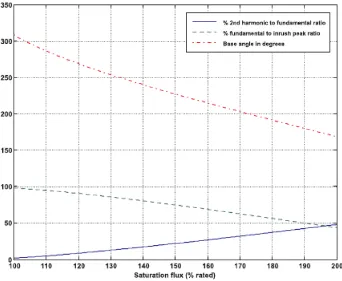
As explained in background that saturation flux plays important part in inrush current magnitude. The B-H curve of the core material and design shows the saturation level. “The base angle of the inrush current is a monotonically decreasing function of the residual flux.” (Wang & Hamilton 2004). Therefore with decrease in saturation flux causes fundamental where increase in saturation flux causes the increase in DC offset and hence increase in second harmonics.

[image:42.595.146.488.241.522.2]

Figure 3.5.1: Saturation flux v/s inrush current (Wang & Hamilton 2004)

Figure 3.5.2: Effect of core saturation on secondary voltage (ElectronicsTeacher.com)

(43)

Page 29 3.2.5 Core material

[image:43.595.231.408.328.457.2]

Magnetic properties are related to atomic structure. Each atom of a substance, for example, produces a tiny atomic-level magnetic field because its moving (i.e., orbiting) electrons constitute an atomic-level current and currents create magnetic fields. For nonmagnetic materials, these fields are randomly oriented and cancel. However, for ferromagnetic materials, the fields in small regions, called domains (as shown below), do not cancel. (Domains are of microscopic size, but are large enough to hold from 1017 to 1021 atoms.) If the domain fields in a ferromagnetic material line up, the material is magnetized; if they are randomly oriented, the material is not magnetized.

Figure 3.6: Random orientation of microscopic fields in a non magnetized ferromagnetic material

(44)

Page 30

Figure 3.7: Field intensity v/s change in the domain orientations. H I

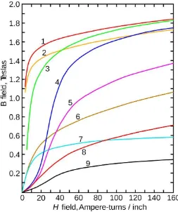
[image:44.595.191.444.421.723.2]

For ferromagnetic materials, is not constant but varies with flux density and there is no easy way to compute it. In reality, however, it isn’t  that we are interested in: What we really want to know is, given B, what is H, and vice versa. A set of curves, called B-H or magnetization curves discussed in earlier section, provides this information. (These curves are obtained experimentally and are available in various handbooks. A separate curve is required for each material.) The figure 3.8 shows typical curves for various materials.

(45)

Page 31

Figure 3.9: Field intesity v/s Permeability and Flux density

[image:45.595.187.449.73.284.2]

In core type transfors the windings are wound around each limbs. The general arrangement is as shown in figure 3.10.

Figure 3.10: Example of core section length

It is clear from the above figure that the lib of centre phase is shorter then remaining two phases. The reluctance of the core is directly proportional to the length of the material. Hence for the given flux density the limb of centre phase will have less reluctance compared to the other two limbs.

3.2.6 Supply/Source impedance

(46)

Page 32 smaller impedance than that of transformer causes the inrush current to be limited. This will also cause system voltage drop which is harmful to house/office hold electrical and electronics equipment’s. (Seo & Kim 2008) The distance between supply source and transformer is also indication of longer busbars/transmission lines. This indicates additional resistance which contributes to damping of the current. The transformer away from the supply with higher line/busbar resistance has shorter inrush currents in duration compared to the ones which are closer to the generating units (Al-Khalifah & Saadany 2006)

3.2.7 Loading on secondary winding

The load on the transformer secondary side has no effect on the inrush of primary current. There are number of authors who claim that this is not the case. The testing done by [34] shows that the load (resistive or inductive) on secondary winding of the transformer has no influence on the inrush current of primary. “The reason for this feature is that when the transformer is saturated, the current peak mainly depends on the slope in the nonlinear zone of the saturation curve.” (Moses eta al 2010)

3.2.8 Size of transformer

(47)

Page 33

3.3 Effect of inrush current

3.3.1 High starting current

When a transformer is energised from a standard power source it draws high starting current which can be as high as 10 – 100 times of transformer’s rated current. This current will starts to decay at the rate of effective winding resistance and will settle down to steady state condition. The time to decay can be as long as few seconds. This current is known as magnetising inrush current (Naghizadeh et al 2012). This effect is described in section 3.1 and section 3.2.

3.3.2 Voltage distortion (harmonics)

Transformers power quality performance in distribution system is the key performance indicator. Switching due to alteration or load is continuously required and due to this it invites problems like inrush current which is rich of harmonics (Seo & Kim 2008). The figure 3.11 shows a spectrum of harmonics and their magnitude derived by Ashrami and others (2012).

Figure 3.11: Spectrum of harmonics in inrush current (Ashrami et al 2012, p.537)

(48)

[image:48.595.221.421.73.193.2]

Page 34

Figure 3.12: Harmonics contents of the idealised inrush current (Kulidjian et al 2001)

When a transformer is energised, due to large inrush current, it also caused the voltage drop especially when transformer impedance is smaller than that of source impedance (Seo & Kim 2008). Such effect can be very sensitive to the some industrial customers and house hole/office electrical equipment. For this reason the calculation of inrush current, voltage drop and harmonics is important. The balanced three phase system the equitation of voltage drop is given by Vaddeboina et al (2012),

Where Vd =voltage drop

m = change in load in kVA

S = short circuit level in MVA

(49)

Page 35

Figure 3.13: Simulated RMS Voltage in kV v/s time in seconds (Vaddeboina et al 2012)

3.3.3 Sympathetic inrush

(50)

Page 36

[image:50.595.225.409.381.533.2]

Figure 3.14: Inrush currents v/s sympathetic inrush currents (Vaddeboina et al 2012)

Sympathetic inrush current can be as high as normal inrush. Due to this effect the importance of transformer differential protection and other protection study for nuisance tripping becomes vital. T

Figure 3.15: System strength v/s sympathetic reaction (Bronzeado & Yacamini 1995)

3.3.5 Vibration/geometric movement of winding

(51)

Page 37 problems transformer manufacturers accounts for strong structure which holds the winding and core tightly (Steurer & Frohlich 2002).

In a number of discussions it was argued that what (inrush or short circuit) is the worst in terms of electromechanical forces. During the discussion it was pointed that the short circuit last for only few milliseconds as protection system isolates the faulty circuit, where the inrush current last for 10s of seconds. The frequency of occurrences of inrush is far more than short circuit faults too. It was also discussed that the magnitude of current are near similar to each other when transformers are energised at no loads. (Steurer & Frohlich 2002)

Transformer energised during no load exhibits large inrush current which causes unbalanced magneto motive forces and transformer core saturation. (Steurer & Frohlich 2002) This leads to large axial forces on windings. Such forces are much higher in the range of two - ten times compared to the forces generated during short circuit conditions. The key difference between the inrush current and short circuit current however, is the forces on secondary side of the transformer. During inrush condition no or very small amount of current and hence forces being generated, where, in short circuit condition the both sides of the windings are equally(or according to % ratio) loaded and affected due to electro-mechanical forces.

The equitation of the local force density in a coil is given by

Where J = current density

B = flux density

During the inrush of current and short circuit of a transformer generates two main types of forces acts on the winding. These forces are square of current.

RADIAL FORCE

(52)

Page 38 while outer winding, like inrush current, gets stretched. The radial forces during short-circuit are more harmful than that of inrush current. (Neves et al 2011). Please referrer to the figure 3.16 for clarification.

Figure 3.16: Radial forces during inrush and short-circuit conditions (Neves et al 2011)

AXIAL FORCE

The axial force compresses the winding towards the ground means the forces pushes the winding downwards. The force during inrush current is higher than short-circuits as flux during transformer energization is higher. (Neves et al 2011) The inrush current generates axial force only on the winding being energised however the short-circuit, as current flows through both windings, generates axial force on both primary and secondary windings. Please refer to the figure 3.17.

(53)

Page 39 3.3.6 Protection complexity - Actual fault v/s Inrush current

As discussed in earlier chapter, in B-H curve, to generate any flux higher than knee point a large amount of current is requires as core trends to saturate exponentially.

The general equitation of inrush current that provides amplitudes of current over a function of time is as shown below, .(Apolonio et al 2004)

√ ( )

Where =maximum applied voltage

=total impedance under inrush

=constant for 3 phase winding connection

=constant for short circuit power of network

=energization angle

=core saturation point

=time

=time constant of transformer winding under inrush conditions

However, for the purpose of protection system design the most important factor remains the peak magnitude of inrush current.(Apolonio et al 2004) The much simplified version of equitation for peak value calculation is derived as shown below, √ √ ( )

Where =maximum applied voltage

L =air core inductance

R=total dc resistance

(54)

Page 40 =residual flux density

=saturation flux density

It is clear from above two equitation that the inrush current depends on mainly residual flux and switching angle. (Apolonio et al 2004)

Figure 3.18: Sample inrush current (Kulidjian & Kasztenny 2001)

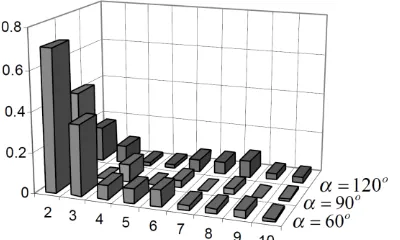
Figure 3.19: Ratio of second harmonics to fundamental (Kulidjian & Kasztenny 2001)

(55)

[image:55.595.125.533.171.734.2]

Page 41 The algorithm (figure 3.20) developed by Hooshyar (2012) has same principle however, instead of calculating direct harmonics contents, the waveform correction scheme and odd and even part extraction methods are used to differentiate the inrush current in actual internal fault.

(56)

Page 42 The wave form of fault current is full wave but of higher magnitude. This waveform will be close to sine wave. However, the waveform of inrush current is not sine wave. It has DC components and it is half and peaky wave. The difference is as shown in figure 3.21 and figure 3.22. A paper presented by Rehmati and Sanaye-Pasand (2008) shows that transformer fault and inrush can be distinguished by wavelet transform.

[image:56.595.180.458.208.422.2]

Figure 3.21: The fault current v/s inrush current waveform (Rehmati & Sanaye-Pasand 2008)

Figure 3.22 : Idealised inrush current (Kulidjian & Kasztenny 2001)

3.4 Inrush current mitigation techniques

3.4.1 Asynchronous switching v/s Inrush Current

(57)

1/-Page 43 1pu. However, this exercise can create other problems depending on the connected at downstream of the transformers. It was also noted that the operation can be expensive as exchange of line breakers were necessary.

Asynchronous switching is turning each phase circuit breaker at separate time instead of same time. In start connected primary of transformer, when asynchronous switching takes place, during the first phase switch all current goes from first phase winding to neutral. (Cui 2005)This current is negative sequence current. During second phase switching the neutral current can be even greater than that of second phase as first phase also contributes to the neutral current. However, then third phase is energised the negative sequence current comes to zero instantly.

3.4.2 Neutral Earthing Resister v/s Inrush Current

[image:57.595.122.518.496.713.2]

A practical done by (Cui 2005) on transformer reveals that the optimal neutral resister can be derived from simulation and is as effective as series resistance/voltage divider method and can significantly reduce the inrush current magnitude and duration. The figure 3.23 and 3.24 shows the optimum value of NER is 50ohm based on calculations and analysis done on 225kVA, 2400/600V, 50Hz 3ph, YY transformer.

(58)

[image:58.595.174.462.67.562.2]

Page 44

Figure 3.24: Inrush current v/s value of neutral earthing resistors (Hajivar 2010)

The equitation derived by Xu et al (2005) for the optimum value of the resister is,

Where, =Neutral earthing resister and

(59)

Page 45 (Xu et al 2005) suggests that about 1 quarter of circuit breaker contact voltage and up to 90% reduction of inrush current can be achieved by switching the pole sequence as A, B & then C.

The neutral earthing resister limits the current going to neutral which limits the inrush of current during first and second phase energisation.

Figure 3.25: The value of neutral earthing resister and effect on inrush current (Cui et al 2005)

3.4.3 Comparison of various methods

(60)

Page 46 the main primary circuit breaker. This method is derived from so called reduced initial primary voltage.

(61)

Page 47

4.

Methodology

This chapter contains information about the number of inrush current effects and the construction of the model. It describes the list of simulation scenarios and, the specification of an actual transformer and running data history, modelling software, brief on model, parameter used in model, the sketch of model and finally measurement techniques. The chapter basically presents the methodology of constructed models and simulated scenarios.

When a transformer is energised from a standard power source it draws high starting current which can be as high as 10 – 100 times of transformer’s rated current. This current will starts to decay at the rate of effective winding resistance and will settle down to steady state condition. The time to decay can be as long as few seconds. This current is known as magnetising inrush current (Naghizadeh et al 2012). This effect is described in section 3.1 and section 3.2. The inrush current results in nusence trip of protection system, it generates second harmonics creating power quality issue, and added mechanical stress due to high magnetic forces generated due to such events and due to all of above it negatively affects the life of a transformer.

The listed following simulation effects are based on above principle.

4.1 List of scenarios

- Inrush current compared to actual transformer

(62)

Page 48 - Inrush current in 3 single phase and a 3-phase transformer

After comparing above model with actual transformer a 3 single phase transformer model will be created that matches all relevant power parameters of 3-phase transformer model. The results of 3-single phase transformer model simulation will be compared with 3 phase transformer model. The discussion and conclusion will be derived according to the findings.

- Sympathetic inrush current

This inrush current flows when two or more transformers are connected together in parallel. Sympathetic inrush flows to the transformer which is already energised when another new transformer on same parallel line is energised. Due to inrush on new transformer the remaining connected transformer will feed the necessary current (as impedance goes down). This effect will be simulated by connecting a number of transformers in the system and switching a new transformer on the system. The magnitude and duration will be a key focus in this simulation result.

- Sequential phase energisation (with/without NER)

(63)

Page 49

4.2 Modelling package

SimPowerSystem is specially designed Simulink block library that has all necessary power system components. This system was developed by Hydro-Quebec of Montreal. “SimPowerSystem models are assembled as a physical system. Models are connected by physical connections that represent ideal conduction paths. This method of modelling being physical and schematic it is easier to understand while at backend the system automatically constructs the differential algebraic equations (DAEs) that characterize the behaviour of the system and integrates with the rest of the model”. (Mathworks NDT)

4.3 Measurement techniques

The three phase voltage and current is measured using a VI meter as modelled below. The Fast Fourier Transformation reveals the harmonics contents and magnitude. The time of inrush current decay is also noted.

Figure 4.1 : Three phase V, I and IFFT scope

4.4 Existing arrangement

(64)

Page 50 terminal via an AVR and three single phase

√ transformer rated 2.2MVA.

[image:64.595.180.460.150.634.2]

Generator is star connected and neutral is grounded via a neutral earthing transformer and 5.6Ohm resister.

(65)

Page 51

4.5 Actual data sourcing

High speed data is be sourced from the IDM-Hathaway unit. The device has already captured varieties of different data from various system disturbances to new start and shutdown event etc. This data from the date file will be converted to appropriate file format to import in to Matlab simulation program.

IDM(HATHAWAY)

IDM-Hathaway is electrical fault recorder. It is a well-known brand in large electric power stations. This recorder in the event of any system disturbances captures the high speed data triggered according to user defined settings. “The product, when coupled with the Qualitrol Hathaway Replayplus software package, provides a powerful platform for the acquisition, analysis and reporting of data from power systems.” (Hathaway, NDT)

SAMPLE DURATION AND RATE

The existing IDM unit is set to capture 128 samples per cycle for fast data capture. This high speed recorder captures the data for 6 seconds. The settings are done so that it starts recording 1 second pre event and 5 second post event. The second inbuilt recording function is slow speed type. This recorder captures the data at 10 samples per cycle. This data is continuously being recorded however, due to memory issues the data after 3 months gets over written.

4.6 Model subsystems & parameters

(66)

Page 52 curve however the curves were unavailable due to confidentiality issue. Therefore instead of using user defined curves, here a standard more widely referred in Matlab’s curve is used by selecting the transformer as saturable transformer.

The following are the key components of the models that can be used in a subsystem however, for simplification they are left on the main system.

Circuit Breaker Timer

The circuit breaker timer was created to simulate the circuit breaker turning on times. The low voltage side of the transformer was switched on at half second interval and the high voltage side of the circuit breaker was switched on at two seconds interval.

Figure 4.3 : Circuit breaker timing circuit

(67)

Page 53 Transformer Input model

The input model described in figure 4.4 provides the energy to low voltage side of the transformer. This model consists of a three phase generator, V/I sensor, excitation transformer, three phase isolated circuit breaker and a unit transformer.

The three phase synchronous generator generates 20kV voltage and is connected to three phase isolated circuit breaker via a V/I_Meter block. The isolated circuit breaker resembles the actual plants isolated air circuit breaker. They all get the relay signal at the same time however, since they are physically/mechanically isolated from each other the actual contact time varies in order of up to 10 milliseconds in its healthy state.

Figure 4.5: VI_Meter subsystem

(68)

Page 54 transformer is only partially loaded. The unit transformer provides the energy to station’s local load. For actual simulation here the unit transformer is represented as RLC load with active power of 30MW, the inductive reactive power of 6MVARs and capacitive power of 2MVARs.

Main Transformer model

The main transformer is 600MVA, 20kV to 500kV step up transformer. It gets power from synchronous generator, steps up the voltage to 500kV and sends full output to transmission line. The transformer is delta-star grounded with saturable core. All units are described in per unit quantity.

Winding 1; V1: 20,000V, R1: 0.002pu, L1: 0.08pu Winding 2; V2: 500,000V, R1: 0.002pu, L1: 0.08pu Saturation Characteristic: 0,0 ; 0,1.2 ; 1.0,1.2

[image:68.595.116.533.504.730.2]

The details of inrush current model that matlab sim-power system has used is as shown below. The model consist of mainly a s function, couple of lookup tables and switches.

(69)

Page 56 Transformer output model

[image:69.595.135.500.192.407.2]

The output model described in figure 4.7 provides the energy to load from high voltage side of the generator transformer. This part of model consist of a HV circuit breaker and load that is represented by a similar size step down transformer and load as RLC load at both LV and HV side of the transformer.

(70)

Page 57

5.

Result & Discussion

This chapter contains details about each model, the results and discussion. As described in methodology here mainly five models are built and simulated for analysis of inrush current effect. The conclusion and outcome will be listed in the next chapter.

The computer used here has 64bit i7-2620 CPU with 2.70GHz speed and 8GB RAM that runs on Windows 7 operating system. The Matlab version 7.10 (R2010a) with Simulink 7.5 and SimPowerSystem 5.2.1 is used. The model takes significant amount of processing power and time to simulate each scenario.

The first model described in section 5.1 is a base model. It basically consist of a three phase generator, three phase isolated circuit breaker, the 600MVA generator transformer, a load breaker at output side and grid consist of another transformer and load. The model is simulated at 50Hz and the three phase voltage, current and harmonics are measured and presented on scope. The harmonics content of current for each second is also presented on a separate live figure. This figure automatically runs and updates when model is run.

There are three stages of the switching in each model described in section 5.1 to 5.6. In the beginning of simulation for first 500mS only excitation transformer is in circuit. This transformer is represented by RLC load and hence only small steady state current is seen in the results. At the 500mS interval the generator 3 phase isolated circuit breaker is energised. Here all phases are switched at same time and considered no lag in stitching time. Switching this circuit breaker energises the generator transformer and also unit transformer. Unit transformer is represented as RLC load and hence it has only a small steady state component in power sharing. The output