Practical application of random vibration signal analysis on structural dynamics

Rochester Institute of Technology

RIT Scholar Works

Theses

Thesis/Dissertation Collections

1994

Practical application of random vibration signal

analysis on structural dynamics

Yu-Chin L. Allen

Follow this and additional works at:

http://scholarworks.rit.edu/theses

This Thesis is brought to you for free and open access by the Thesis/Dissertation Collections at RIT Scholar Works. It has been accepted for inclusion

Recommended Citation

PRACTICAL APPLICATION OF RANDOM

VIBRATION SIGNAL ANALYSIS IN

STRUCTURAL DYNAMICS

Yu-Chin L. Allen

A Thesis Submitted in Partial Fulfillment

of the Requirements for 'the Degree of

Master of Science

in Mechanical Engineering

Approved

by:

Professor

J. S.

Torok (Thesis Advisor)

Professor N. Berzak

Advisor D. S. Aldridge (AC Rochester)

Professor

C.

W. Haines (Dept. Head)

Department of Mechanical Engineering

College of Engineering

Rochester Institute of Technology

Rochester, New York

PERMISSION GRANTED:

I, Yu-Chin Allen hereby grant permission to the Wallace Memorial Library of the

Rochester Institute of Technology to reproduce my thesis entitled Practical

Application of Random Vibration Signal Analysis in Structural Dynamics in

whole or in part. Any reproduction will not be for commercial use or profit.

May 17, 1994

Acknowledgements

I

would

like

to

thank

my

family,

my

husband

Stu

for

all

his

patienceand

understanding

over

the

past six years as we endeavored

to

juggle

our work,

school,

and

family.

Our

children,

Russell

and

Susan,

for

behaving

so

I

could work and

encouraging

me

to

finish

so we can play.

I

would also

like

to thank

Dr. Torok for

all

his

support,

countless

Abstract

The

use of random signal analysis

in

vibration and structural analysis

is

discussed

and

documented.

The

need

to

minimize product performance and

durability

risks

due

to

competitive pressure

in the

marketplace

has forced

industry

to

streamline methods of product

design,

processing,

and evaluation.

Engineers

need

to

be

experienced

in

much more advanced

techniques than

they

did

even a

decade

ago.

Random

vibration signals are used

to

simulate real

world environments and are another

tool

in

structural analysis.

This

investigation

outlines

the

basics

of random

vibrations,

frequency

analyzers,

data

analysis,

along

with associated noise and errors problems.

A

case

study

using

an aluminum

beam

is

used

to demonstrate the

concepts presented

in

this

Table

of

Contents

Paae

List

of

Symbols

vii

List

of

Tables

ix

List

of

Figures

X

1.

Introduction

1

2.

Background

4

2.1

Fourier

Analysis

5

2.2

Modern

Frequency

Analyzers

9

2.3

Noise

and

Error

9

3.0

Random Vibration

10

3.1

Basic

Probability

and

Statistics

in Random

Vibration

10

3.2

Correlation

16

3.3

Random Environment

Definitions

17

4.0 Data Analysis

22

4.1

Frequency

Analyzers

22

4.2

Measurement Functions

23

4.2.1

Time Domain Analysis

23

4.2.2

Amplitude Domain Analysis

23

4.2.3

Frequency

Domain

Analysis

24

5.0 Noise

and

Error

27

5.2

Fourier

Transform Algorithm

Error

28

5.3

Error

Classification

32

5.4

Noise

33

5.5

Frequency

Response Errors

40

5.5.1

Random Errors

in

Frequency

Response

40

5.5.2

Bias Errors

in

Frequency

Response

41

6.0

Theoretical

Analysis

43

6.1

Exact

Solution

of

Free

Vibration

43

6.2

Approximation Method

56

7.0

Experimental Analysis

66

7.1

Equipment

66

7.2

Damping

Analysis

67

7.3

Spectral Analysis

and

Correlation

70

7.4

Mode

Shapes

77

8.0

Conclusion

80

8.1

Theoretical Analysis Application

80

8.2

Conclusions

and

Recommendations

88

List

of

Symbols

F(t)

Fourier Transform

Frequency

CO

T

Time Period

p(x)

Probability Density

Function

Standard

Deviation

E

[ ]

Expected Value

RxxCO

:

Autocorrelation Function

Rxy(T):

Cross

Correlation Function

Gxx(T):

Autospectral

or

Power

Spectral

Density

(one sided)

Gxy(T):

Cross

spectral

Density

(one sided)

Sxx(T):

Autospectral

or

Power

Spectral

Density

(two sided)

Sxx(T):

Cross

spectral

Density

(two sided)

H(f)

Frequency

Response Function

2

Yxv(f)

J

Coherence

Function

Be

Filter

Bandwidth

u(t)

True

Input Signal

n(t)

:

Output Noise

M

Moment

V

Shear Force

P

Mass

Density

A

Area

H

Mass

per

Unit

Length

KE

Kinetic

Energy

U

Potential

Energy

D

Dissipation Function

Qi

Generalized Force

[M]

:

Mass

Matrix

[C]

:

Damping

Matrix

[K]

:

Stiffness

Matrix

1>i

Normal

Mode

qi

Generalized Coordinate

nd

Number

of

Averages

?

i

List

of

Tables

Table

Page

Table

1

:

Typical Values

of

S(f)

and

G(f)

21

Table

2:

Determination

of

Log

Decrement

67

Table

3:

Determination

of

Damping,

C

68

Table

4:

Comparison

of

Natural Frequencies

80

Table 5:

Frequency

Response Estimates for Mode

2

84

Table

6:

Frequency

Response Estimates

for Mode 3

84

Table

7:

Frequency

Response Estimates for Mode

4

84

Table

8:

Frequency

Response Estimates for Mode 5

85

Table

9:

Frequency

Response Estimates for Mode 6

85

Table

10:

Frequency

Response

Gains

from Experimentation

85

Table

1 1

.

Frequency

Response

of

First

Mode

Approximation

with

Six

Functions

at

Ten

times the

Damping

Constant

88

Table

12:

Frequency

Response

of

First

Mode

Approximation

with

Six

List

of

Figures

Figure

Page

1

Periodic

Signal for Fourier Transform

Example

6

2

Fourier Transform Example

8

3

Random Signal

1 1

4

Probability Density

Curve

1

2

5

Random Signals

Time Aligned

16

6

Typical Random Vibration Spectrum

20

7

Analyzer Block Diagram

22

8

Waterfall

Analysis Example

26

9

Sine

Wave for Fourier Transform Example

28

10

Sine Wave

Used in

Discrete

Fourier Transform

30

1 1

Ideal

Single

Input/Single Output System

33

12

System

with

Noise

at

Input

and

Output

35

13

System

Model

with

Noise

at

Output

Only

38

14

Beam

Model for

Continuous

System

42

1

5

Mode

Shape

1

with

Exact Solution

52

1 6

Mode

Shape

2

with

Exact Solution

52

1 7

Mode Shape 3

with

Exact

Solution

53

1

8

Mode

Shape

4

with

Exact

Solution

53

1

9

Mode

Shape

5

with

Exact Solution

54

20

Mode Shape

6

with

Exact Solution

54

1.0

Introduction

Fierce

competition

in

the

worldwide marketplace

has forced

industries to

revolutionize

their

processes.

From

concept selection

to

design,

prototype

fabrication

to

mass

production,

every

phaseof a product

has

been

scrutinized and waste of

any

form

(material,

process,

overhead)

eliminated.

No longer

does

industry

have

the

luxury

of

long

lead

times,

oligopolies,

and product

recalls.

Consumers

are

better

educated,

have

more

choices,

and will not

accept a second rate product.

Industry

relies on engineers

to

be

able

to

produce

functional,

durable,

esthetically pleasing

products which perform

better

than the

competition

in

order

to

stay in business.

To stay

ahead of

competition,

the

engineer must make use of

many

tools

available

to

streamline

the job.

The

invention

of

the

integrated

circuit

(IC)

has

given

today's

engineer

important

tools.

Made

available

to

the

masses are reliable and affordable

analyzers,

data

loggers,

sensors,

and computers as a result of

the

IC

revolution.

No

longer

does computing

power reside

in the

halls

of universities and government research

labs.

Powerful

computing

is

available even

to

the

smallest contract

engineering firms

and

engineering

students.

Now

we are able

to

redesign and

improve

product without

hundreds

of

costly

hardware iterations.

One

role engineers must

play in

today's

marketplace

is

that

of

the

appropriately

in the

field

to

guarantee success.

Products

must withstand

their

everyday

use without

cracking,

buckling,

or

failing

their

performance.

There

are

many

tools

available

to the

analyst

today.

Theoretical

analysis and

modeling

are enhanced

by

computers armed with sophisticated software packages which are able

to

solve systemsof complex equations

in

seconds.

Traditional

transducers for

force,

acceleration, pressure,

temperature,

etc. are

complimented with computers and various

analyzers,

which aid

in

defining

the

product and

its

field

of operation.

The

structural

dynamics

analyst

is

responsible

for characterizing

a product's

dynamic behavior in every

appropriate environment.

This

makes

today's

product

better

suited

for fierce

competition.

Random

vibration analysis

is

used

by

the

structural analyst

in

many

ways.

Many

environments products are subjected

to

are considered

random,

such as

the

beating

of waves on oil

rigs, to the

noise

emanating from

automobiles.

A

random environment simulation

in

product evaluation

is

instrumental in predicting

and

assuring durability.

Random

vibration

is

also

used

in

excitation of products

to

determine

dynamic

characteristics,

such as

the

natural

frequency,

mode shapes and

damping

factor.

A thorough

understanding

of random vibration

is invaluable

to the

analyst.

The study

of random vibration

is

not

trivial.

This type

of environment

is

not

simply

described

with

just

one or

two words,

but

through

the

definition

of

varying

frequency

spectra.

To describe the

environment

acceleration,

frequency,

and statisticsmust all

be

utilized.

This

is

usually

done

with

dynamic

characterization of

the environment,

_{and simulation are all possible with}

sophisticated computer systems which

involve

analog- to-

digital

_conversions

(A/D),

signal

processing,

and

Fast Fourier Transforms (FFT). The

terms

correlation and spectral analysis are used used

to

describe

the

randomness of

the

data

and

the

environment.

All

of

this

is necessary

to

understand

the

random vibration environment.

As

with

any

measurements

taken

with sophisticated

equipment, the

question arises as

to the

validity

of

the

data. The

popular adage "garbage in-garbage

out"

has haunted every data

taking

engineer.

Especially

with random

vibration where noise can

look just

as viable as

the

environment

itself,

care must

be

taken

in the

winnowing

process

to

separate

the

data

from

the

noise.

Much

work

has

been

done

in

the

field

of random vibration

to

mentor

the

inexperienced.

The

goal of

this thesis

is

threefold.

First,

random vibration

basics

are

detailed,

and

their

use

in

structural

dynamics

analysis

demonstrated.

Second,

noise and error when related

to

random vibration and signal

processing is

detailed.

Third,

the

concepts are all

tied

together

and

demonstrated

in

an

example

involving

a

beam.

An

aluminum

beam is

presented,

which

is

evaluated

using

several

different modeling

techniques.

The beam is

then

subjected

to

a rigorous

dynamic

evaluation,

and

the

resultscompared

to the

various models.

Recommendations

to

aid

in further

work with

both

random vibration and signal

2.0 Background

The

powerful

Integrated

Circuit

(IC)

revolution

has

changed

the

job

of

engineers.

No longer bogged

down to

solve complicated

third

and

forth

order

equations and

systems,

computer programs are available

to determine the

behavior

of components

through

modeling

only theorized

twenty

years ago.

Finite

element analysis

is widely

used

by industry

to

model complex systems

and

improve designs

without

wasting

valuable

time

physically

evaluating

hardware iterations.

This has

spawned

the

branch

of

engineering

called

computer aided

engineering

(CAE).

The

area of

test

and measurement

has

also prospered with

the

IC

revolution with

the

introduction

of affordable signal

processing

and analyzers.

1

970

marked

the

year of

the first commercially

available

FFT

analyzer

by

Time Data Corporation.

General Radio Corporation

was

instrumental in

developing

the

algorithms used

today

to

create random vibration

in

the

laboratory.

Virtually

any

type

of vibration environment can

be

recreated

in the lab from

mixed mode vibration

to

triaxial

shaker excitation.

Today

the

market

is

supplied

by

many

manufacturers of analysis and

test

equipment who compete

for the business

of structural

dynamics

analysts.

The

IC has

replaced

the

once expensive

analog

computer and

filter

equipment

available

to

the

engineer with affordable

high

speed

digital

ones.

Random

vibration

is extensively

used

in engineering

to

describe

environments.

With

random

vibration,

the

exact values cannot

be precisely

determined for

a given

instant

of

time.

Instead,

a

statistically

valid estimate of

random vibration

involves probability

as well as

its

application

to

measurements.

Many

events are

described

by

random

signals,

such as

jet

noise and earthquake

intensity,

since

there

is

no

deterministic

model

that

can

describe

the

unpredictable nature of

the

events.

Random

vibration can also

be

used when

studying

the

dynamics

of a system.

Using

random

vibration,

all

frequencies

in

a predetermined

frequency

bandwidth

can

be simultaneously

_excited.

This

_{can provide a quick method of}

identifying

natural

frequencies

of

the

system

by

examining

the

system

input

and output.

All

natural

frequencies

are excited at

once,

which allows

the

interactions between

them to

be

examined.

To

the

structural

dynamics

analyst,

this

can

be

of vital

importance

when resonances

have destructive

interference

in

a random vibration environment.

2.1

Fourier

Analysis

A

random signal appears as a complex waveform

in the time domain.

It

is

not a

trivial task to

characterize.

Fourier

Analysis

is

used

to

interpret

random

data

since

the

frequency

domain

is

better

suited

to

describe

random

environments.

The

assumption

is

made

that

all motion can

be described

in

terms

of sines and cosines of

varying frequencies

which are

harmonically

related.

This

was

discovered first

by

J. Fourier

(1768-1830).

Functions

are

described

by

the

period and associated

amplitude,

which are combined

to

create

the

Fourier

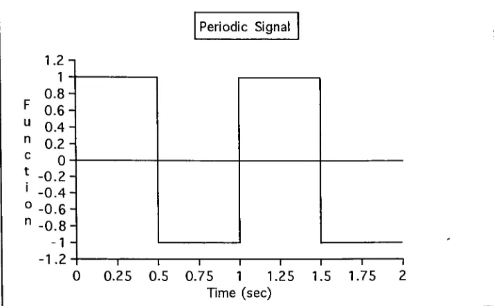
series.

For

an

example,

consider

the

periodic waveform

in

Figure 1.

The

Fourier

series used

to describe the

signal consists of

the

Periodic Signal 0 n c * -0. 1 -0.

-0.

n-0

.2 1 |.4-0

z-\

4 6- 8-1

-1.2 1 1 1 1 1 1 1 1

0 0.25 0.5 0.75 1 1.25 1.5 1.75 2 Time

(sec)

Figure

1.

Periodic Signal Example

for Fourier Transform

Example

F(

l)

:= a

0

+

X!

(a

COS

("'

W 0'

*)

+

b

n sin

(n"

_< 0'

l))

where:

2-_jr.

co

q

:=

T

=

fundamental

frequency

[image:17.548.95.452.44.265.2]

T

F(

t)-sinfn-co0-t)

dt

For the

example presented

in

Figure

1

:

ao

=

an

=

0

n

"

T

~2

F

q-sin

in

(

n-co

q-t)

dt

bn

:- _-F0-(i

-cos(n-co0--T-n-co

0

b

n

'=

F

q-

(l

cos

(n-

k)J

n-n

n 'r

0

n^

jt

^0

F(t)

:=4-31

g(l-sin(nco0T))

F(t)

=4-ji

sin

(

co

q-tj

+ sin(3-co

q-t)

+

-sin(5-co

q-t]

+

1 -I

0.9-F

0.8-u

0.7-n

0.6-c 0.5-*

0.4-1

0.3-0.1

-

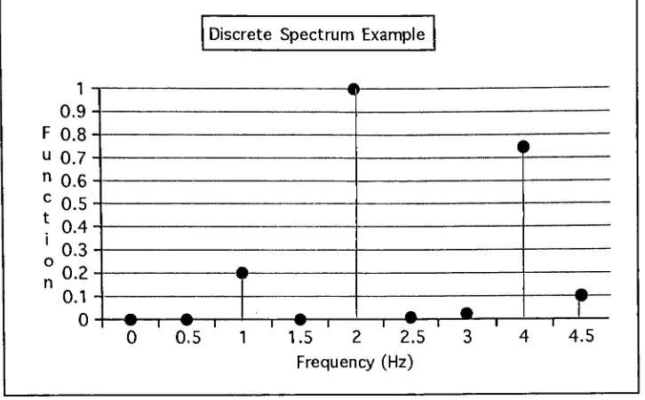
0-Discrete Spectrum Example

* t

%t

m

A

T

0 0.5 1 1.5 2 2.5

Frequency (Hz)

1 1

3 \ 4.5

Figure

2:

Fourier

Transform Example

The

operation

itself is

quite

laborious

and prohibitive when performed

by

hand

on a complex

signal,

but

has

been

assimilated

to the

modern computer age

through the

use of

Discrete Fourier Transforms

(DFT)

where

large

sets of

data

can

be

manipulated

using

this

algorithm on computers.

The Discrete Fourier

Transform

is

an approximation of

the

continuous

Fourier

transform:

X(f)

:= 00

-00

x(t)-e"j23tftdt

[image:19.548.101.464.24.249.2]

x

1 -j2scf( ndt)

In

1965

J. W.

Cooley

and

J. W.

Tukey

introduced

a new method

for

determining

coefficients,

involved

with

Fourier

transform

algorithm,

which

greatly

reduced

the

number of

data

points needed.

This is

the

Fast Fourier Transform

(FFT)

which

forms

the

basics

for

much of

the

computations

in

equipment

today

.

For

more

information

on

DFT

and

FFT

see references

2

and

7.

2.2

Modern

Frequency

Analyzers

Today,

the

dynamic

signal analyzer

is

a

basic

tool

used

by

anyone

studying

structural

dynamics.

Analyzers

can

be

multichannel,

allowing for the

investigation

of multiple

inputs

simultaneously.

Not only

can

the

motion of a

single point

be

determined,

but

the

interactions between

points can

be found.

Time

and

frequency

domain

measurements are made

in

a matter of seconds.

Analyzers

are

flexible;

parameters are manipulated

to

suit

the

data

under

investigation.

If

peaks value are

the

main

interest

of

the user, then

averaging

techniques

and

windowing

are

easily

manipulated

to

reflect peak

hold

data

and

flat

top

windowing.

Data

is

stored

in basic formats for

transfer

into

spreadsheets

for

more complex mathematical manipulation

through

standardization of

file

formats

such as

the

Universal

File

Format

(UFF)

or

Standard File

Format (SDF).

Manipulation

of

data

is

not aroadblock

for

today's

engineer.

Armed

with

the

appropriate

transducer,

signal

conditioning,

and

analyzer,

engineers can make

2.3

Noise

and

Error

Noise

and error plague

engineering

data.

Sophisticated

equipment

is

haunted

by

ubiquitous power

line

noise

(usually

60-Hz).

The

most meticulous of measurements can

be

destroyed

by

a

noisy

environmentor errors.

The

recognition of errors and noise and methods

to

affect

them

are

necessary to

assure viable

data.

Simple

techniques

exist,

such as

increasing

statistical

accuracy

by

increasing

the

number of measurements used

in

averages,

which must

be

weighted against

the

cost of

doing

so

in

the

competitive marketplace.

It

is

difficult

to

obtain several samples of a one

time event,

such as

the

launching

of a satellite.

Engineering

judgment

must

be

relied on

to

make a

"good

enough"

3.0 Random Vibration

Random

vibration

is

a vital part of

the

analysisof

dynamic

systems.

A few

applications of

the

concept of random vibration are: resonance

identification,

modeling

of complex

systems,

description

of realistic environments.

Definition

of

basic

terms

used

to

describe

random events

is

needed

before proceeding

further

into

correlation and spectral analysis.

Random

signal analysis

is

used

to

identify

situations

in

which precise values

cannot

be determined

to

identify

the

system,

so

best

estimation

is

used.

Probability

and statistics are needed

to

describe

the

properties of

the

environment .

The study

of random vibrations

deals

with

determining

the

statistical characteristics of a system and

how

the

output

depends

on

the

dynamic

properties of

the

system under

investigation. Several terms

are

needed

to describe

a random

signal,

such as

average,

mean

square, variance,

and correlation.

To

understand

them,

a

brief introduction to

a

few

concepts

in

statistics will

be

presented.

3.1

Basic

Probability

and

Statistics in

Random

Vibration

A

fundamental term

in

statistics

relating

to

random signal analysis

is probability

density

function

(PDF),

which

is

given

the

symbol p(x).

PDF

is defined

as

the

length

of

time

an event occurs

between

two

given

limits

divided

by

the total

length

of

the

event under observation.

PDF

defines

the

probability

an event wil

p(xo)

= _prob

(

x0

<x<

x0

+

dx)

=

dt/T

where:

dt=

the time

xo<x<xrj

_-i-dx

T

=

the total

_{period of}

investigation.

rx

Prob

(x

i<x<x2)

:= p( x)

dx

To

help

understand

the

conceptsof random

vibration,

a random sample can

be

used

to

identify

basic

terms.

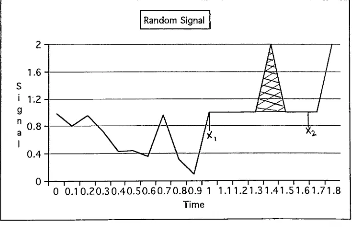
Figure

3

displays

a

typical

random event recorded

over a period of

time.

The probability

that

the

x value will

be

in

the

range of

xi

and

X2

during

the

time

period

T

identified is indicated

by

the

shaded area.

1.6 s

i _1.2 g n

I 0.8

0.4

Random Signal

i i i i i i i i i i i i i i i i i i 0 0.10.20.30.40.50.60.70.80.9 1 1.11.21.31.41.51.61.71.8

Time

[image:23.548.101.462.379.614.2]

For

the

example

if the

period

is between

1

and

1

.6

for the time

period,

and

the

probability

that the

signal

is

greater

than

1

for

the

identified

time,

then:

T

= 1.6-

1

_=0.6

dt

=

0.2

(shaded area)

then

:

p(x)

=

.2

/

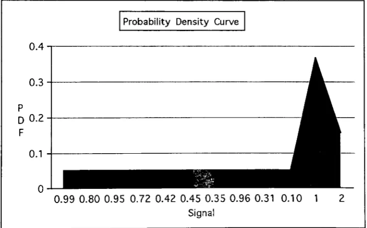
.6 = .33.

A

Probability Density

Curve

is

a plot of

PDF

vs.

the

event .

See

Figure

4

for

an example.

The

area under

the

probability

density

curve gives

the

probability.

Referring

to the

example set

in

Figure

3,

the

probability

the

x value

being

between x-|

and

X2

during

the time

period

T

is

shown

by

the

shaded

region

in

Figure

4.

The

probability

density

curve portrays

the

probability

of x

without

the

time dependence.

Probability Density

Curve

0.4

0.99 0.80 0.95 0.72 0.42 0.45 0.35 0.96 0.310.10 1 2

Signal

[image:24.548.102.463.352.576.2]

Measurements

of

probability

density

and

the probability

density

curve can

be

made with a

probability

analyzer.

The

event under

investigation

is

sampled

quickly

over a period of

time,

then

displayed.

The

values

for the limits

are

then

entered and

the

probabilities

determined.

Many

naturally

occurring

events,

when sampled over a

long

period of

time,

will

display

a

bell

shaped

curve which

has been been termed

the

Gaussian Distribution.

The

formula

for

the

Gaussian

Distribution is:

-,_(x N2

m)

p(x):=-Lr.e

where:

m = _{mean value of x}

a = standard

deviation

The

Gaussian

distribution is

also referred

to

as

the

normal

distribution.

In

random vibration

theory,

the

characteristics of

many

systems are approximated

by

this distribution.

Random

Environments

are

described

by

a

few

key

formulas,

such as mean value and standard

deviation

which will

be defined

next.

The

mean value

is

a

fundamental

characteristic of

the

environment.

When p(x)

can

be

determined for

a random

process, then

a

variety

of characteristics can

be

defined for the

process

defined

as x(t).

Allowing

the

expression

E

[ ]

to

signify

the

expected value of

the term

in

the

brackets,

the

following

definitions

are

defined:

E[x]

=m=i:-

x(t) dt

Relating

the

p(x)

to the

mean,

since

dt

Zt:=p(x)-

dx

Then

:

E[x]

= 00

-00

x-p( x)

dx

The

mean value gives

the

central

tendency

of a

function

or signal.

Similarly,

the

mean square value of x=

E

[

x

2

]

: average value of x

2

E

[

xA2

]

= x(t)2dl

00

x -p(x)

dx

Standard

Deviation

of

x,

a , and

variance,

a can

then

be defined:

The

variance

is

the

square of

the

deviation

of

the

x

from

the

mean

level

E

[

x

]

.

It

can also

be

shown

that

the

variance

is

equal

to the

mean square

minus

the

mean squares or:

2

a=E[x2]-(E[x])2

Variance

provides an

indication

of

the

dispersion

of

the

variable about

the

mean value.

Now

that the

basic terms

used

to

describe

random processes

have been

defined, they

can

be

used

to

describe

environments.

A

sample

function

is

a

single

time

history

used

to

describe

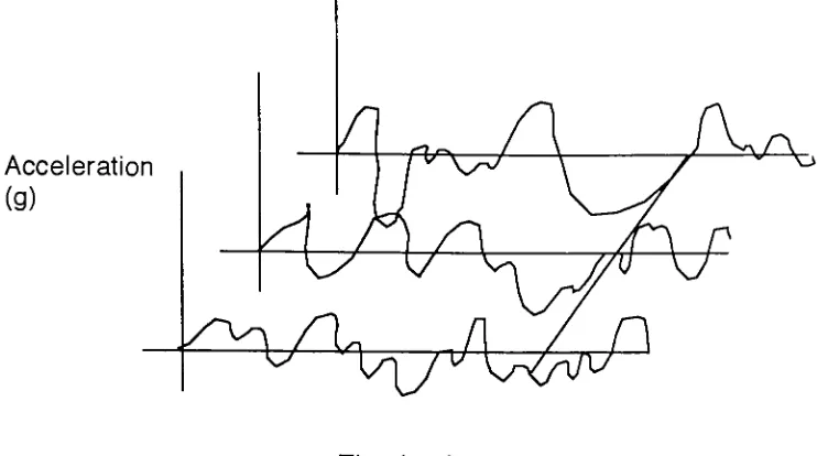
a random process.

A

collection of sample

functions is commonly

referred

to

as an ensemble.

The

mean value of a

sample

function

can

be

found

through

summing the

instantaneous

values of

each sample

function

at

the

same

time point, then

dividing by

the

number of

functions(See Figure

5).

The

term

stationary

random process refers

to

a

process

in

which

the

characteristics

(mean

value and

variance)

of

the

ensemble

do

not

depend

on absolute

time.

Stationary

also means ensemble average

is

Acceleration

(g)

Time(sec)

Figure

4:

Random

Signals

Time Aligned

3.2

Correlation

Correlation is

used

to

determine how

a

function

relates

to

another

function

at a

later

point

in

time.

Two

types

of correlation are

instrumental

to the

study

of random

vibration,

autocorrelation and cross correlation.

Autocorrelation

relates a

function

to

itself

at a

later

fixed

instant

of

time.

The

formula for

Autocorrelation

is:

Rxx(T)

=

E[x(t)x(t

+

T)]

or

RxxW

=lim

1

rT

T_?oo

T

x(

t)-x(t +

x)

dt

[image:28.548.92.463.43.250.2]

1

.

if

the

process

x(t) is stationary,

then the

mean and standard

deviation

are

independent

of

t

2.

it

is

an even

function

For Cross

correlation relates

two

different functions

at a

fixed

later

time:

Rxy(T)

=

E

[

x(t) y(t+T)]

and

Ryx(T)

=

E

[

y(t) x(t+T)]

or

rT

RXy(x)

=

lim

j_.

T-^-oo

T

x(t)-y(t +

x)

dt

In

general,

cross correlation

if

not even.

It

the

time

separation

T is very

large,

no correlation

is

expected.

Correlation is commonly

used

to

detect periodicity

in

functions,

predict signals

in

noise,

and aid

in

the

measurement of

time

delays.

3.3

Random

Environment

Definitions

With

the

definition

of

correlation,

other

terms

used

to

describe

random

vibration can

be

introduced.

A

nonstationary

random process

is

one

in

which

the

mean and autocorrelation

vary

with

time.

The terms weakly

stationary

or

stationary

in the

wide sense

describe

a special case

in

random vibration where

the

mean

is

constant,

but

the

autocorrelation

depends

on

the time

separation

(T)

only

and not

time

(t).

Strongly

stationary

or

stationary

in the

strict sense

implies

that

the

correlation

is

time invariant.

A

nonstationary

random process

has

characteristics which

depend

on

time;

to

characterize

it,

an

instantaneous

where

the

mean and autocorrelation computed

for

asample are

the

same

for

the

entire

function

of a

stationary

random process.

Autospectral

or

Power Spectral

Density

(PSD) (Gxx (0)

for

a

stationary

record represents

the

rate of change of

the

mean square value with respect

to

the

frequency. This

term

is

used

extensively in

describing

random vibration

processes,

as

it

relates

the

vibration amplitude with

probability,

hence it is

instrumental

to

random processes.

The

values are estimated

by

computing

the

mean square value

in

a narrow

frequency

bandwidth

at central

frequencies,

then

dividing

the

value

by

the

frequency

bandwidth.

The

total

of all mean

square values

divided

by

frequency

gives

the

total

area of

the

function

and

is

the

total

mean square value of

the function.

Spectral

density

functions

are

commonly

used

for: determination

of

system properties when random vibration

is

involved,

specification of random vibration

test profiles,

and

identification

of

energy

and noise sources.

Fourier

analysis

ties

together

the time

and

frequency

domains

of a

signal.

The

coefficients of

the

Fourier

series can

be

plotted against

frequency

producing

the Fourier

spectrum.

Computers

are

instrumental in

performing

Fourier

transforms

utilizing

the

fast Fourier Transform

(FFT)

algorithm which

minimizes

the time to

compute values.

X(f)

:= 00

x(t)-e~i2ltftdt

with

the

inverse

transform:

x(t)

:=

00

-00

X(f)-ei2jlftdt

where

the

integral

can

be

considered as a summation of

the

continuous

spectrum of sinusoids.

Spectral

Density

is defined

as

the

Fourier

transform

of

the

correlation

function.

There is

autospectral

density

defined

as:

S(f)

:=

XX Rxx(x)e

l2*fTdx

with

the

inverse:

RxxG)

:=

and cross spectral

density

defined

as:

S

xx(

f)-e

5tT

dx

Sxy(f)

:= 00

R

xy

(x)

e 1 % x

dx

R

xy

(,):=

00

Sxy(f)-ei2:ifTdx

The

units

for

spectral

density

are

the (mean

square value)/

(unit

of

frequency).

Used commonly in

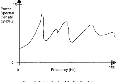
vibration

is

acceleration spectral

density

or power spectral

density

described

as gA2/Hz.

A

graph of a

typical

random environment of

this

type

is

shown

in Figure

6.

The

mean square value of a

stationary

random

process

is

the

area under

this

graph which

is

also

Rxx(O).

Power

Spectral

Density

(gA2/Hz)

0

Frequency

(Hz)

Figure

6: Typical

Random Vibration

Spectrum

Two

common

terms

used

to describe

processes are narrow

band

and

broad band.

As

the

names

imply,

a narrow

band

process

has

spectral

density

which occupies

only

a narrow

band

of

frequencies.

A

broad band

process

consists of a wide

frequency

band

of excitation.

These

types

of processes can [image:32.548.82.476.217.495.2]

range

is known

then

narrow

band

excitation can

be

used

to

excite a small

range.

If there

is

no

indication

of

frequency

range

to

use, then

a

broad band

is

typically

selected

to

provide an

indication

of

further

excitation needs.

If

the

frequency

range of

interest is limited

to

positive

frequencies

only

(

from

0

to

positive

infinity)

then

one sided spectral

densities

are of

interest.

These

are

defined

as

Gxx(

f

)

and

Gyy(

f ):

Gxx(f)

=

2Sxx(f)

andGyy(f)

=

2Syy(f).

in

which

f

>

0.

This is

feasible,

since

S(f)

is

even.

Typical

valuesof

S(f)

and

G(f)

are presented

in Table 1.

Table

1

:

Typical

values of

S(f)

and

G(f)

Frequency(Hz)

S(f)

(gA2/H;_z) G(f)(gA

0 0.002 0.004

5 0.0052 0.0104

10 0.036 0.072

15 0.009 0.018

20 0.6 1.2

25 0.003 0.006

30 0.0025 0.005

35 0.058 0.116

40 0.006 0.012

45 0.0063 0.0126

4.0

Data Analysis

Data

analysis

for the

structural

dynamics

analyst

typically

involves the

frequency

responseof a structure

instrumented

with

transducers.

Basic

terms

and applications are presented

in this

section.

Examples

are

displayed in

Chapter

7

with

the

aluminum

beam

example.

4.1

Frequency

Analyzer

Frequency

analyzers are used

throughout

industry

as a

tool

in

understanding

system

behavior. Whether

the

system

is

a

vibrating

mass or a

production

line

a

dynamic

signal analyzer will make a physical measurement

then

present

it in

a

format

the

user requires.

A

frequency

analyzer consists of a

bank

of variable

frequency

narrow

band filters

with an rms meter

to

display

the

filter

output.

The

first

analyzers

were

analog,

which could

be very

cumbersome and

large

depending

on

the

functions it had

to

perform.

Many

analyzers

today

accomplish

the

filtering

through

digital

signal

processing

(dsp)

chips,

so analyzers can

be

portable

hand held

units.

See Figure

7

for

a

block diagram

of a

typical

frequency

analyzer setup.

Input x(t)

Narrow Bandpass filterw/

bandwidth=dfandcenter frequency=

to.

Square

and

Average

Divide

by

df

Gxx(fQ)

Obtain

x(fo,

df,

t)

4.2

Measurements Functions

Analyzers

are

flexible

instrumentation.

With

the

appropriate

hardware

configuration,

structures as

large

as

buildings

and as small as electronic

boards have

their

dynamic

characteristics

identified.

Three

common

measurement

domains

are

the

time,

amplitude,

and

frequency.

Other

measurements are available as special

features

of equipment _{manufacturers,}

such as

Bruel

and

Kjaer's Cepstrum

analysis.

4.2.1

Time

Domain

Analysis

Time

domain

analysis

usually

consists of a

time

record and

the

autocorrelation and cross correlation

functions

associated with

the

signals.

This

is

the type

of

trace

which can

be

found from

an

ordinary

oscilloscope.

Time

domain

analysis can

be

used as a quick method of

monitoring

signal

integrity.

When starting any

analysis,

a quick view of

the transducer

prior

to

measurement

can

indicate

problems with

instrumentation

setup.

Time domain

analysis

(sometime

a referred

to

as

running mode)

and

operating

mode

deflection

are

two

analysis

types

which

takes

a structure

operating in its

normal condition and

displays

the

dynamics

as a

function

of

time.

It

is distinguished from

modal

analysis,

in

that

it is

time

based

instead

of

frequency

based.

It has

the

ability

to

show product

interactions

during

operation.

Analyzers

start with

data from the

time

domain

to

form

frequency

and amplitude

domain

measurements.

4.2.2

Amplitude Domain

Analysis

Amplitude

domain

analysis consist of

histogram,

probability

density

details).

It

can providean

indication

of

data

nature

(

is it Gaussian

or not

?)

or

give minimum and maximum

data

values over

the

data

record.

This involves

general statistical analysis.

4.2.3

Frequency

Domain Analysis

Frequency

domain

analysesare

important

to

the

structural

dynamics

analyst

in understanding

the

dynamic

characteristics of

the

structure.

Power

spectrum

(both

cross and

auto),

linear

spectrum,

frequency

response,

coherence,

and spectral maps are all

typical

measurements.

Power

spectra

(for

details

see chapter

3)

are

one-sided,

versus

linear

spectra which are

two

sided.

Linear

spectra are

the

result of

direct FFT

of a

time

signal.

Spectral

measurements are useful

in

identifying

frequencies

of

interest

(

resonances,

operating

frequencies,

cutoff

frequencies,

etc.

).

Frequency

response

is

a

two

or more channel measurement.

One

channel

is

typically

designated

the

input,

and all others

the

outputs.

The

frequency

response

function

of a

system,

H(f),

is

defined

as:

H(f)

:=

00

h

(x)

e J

T

dx

where:

h

(

x

)

=

the

unit

impulse

function

describing

the

system

Using

complex polar notation

to

describe

frequency

response:

H(f)

:= |H(f)|-e~j*(f)

I

H(

f

)

|

=gain

factor

of a system

<K

f

)= phase

factor

of a system

H(

f

)

is

the

Fourier

tranform

of

h(x ).

Many

engineers use

the terms

"frequency

response"

and

"transfer

function"

interchangeably. This

should not

be

practiced,

since a

transfer

function

more

accurately describes

the

Laplace

transform

of

the

unit

impulse

response

function.

The

coherence

function

is

also used quite

commonly in the study

of

system

dynamics. Coherence is

the

_{ratio of}

the

absolutevalue of

the

cross-spectral

density

function

squared, to the

product of

the two

comprising

autospectral

density

functions:

^

GXX(f)-Gyy(f)

Coherence is

a measure of

the

accuracy

of

the

linear input/output

model

assumed

for

the

system under

investigation.

Coherence

is

used

successfully

in

identifying

errors,

as will

be discussed in

chapter

5.

Spectral

maps,

or waterfall analyses are a

three

dimensional

displays

of

data.

Typically

anotherparameter, such as revolutions per minute

(rpm)

for

a

rotating

piece of machinery,

is

used

to

align

the typical

power spectrum while

conditions are varied.

This

type

of analysis

is

useful

in

distinguishing

between

system natural

frequency

and

forced

vibration.

A

natural

frequency

will

be

vibration will

vary

following

the third parameter

(rpm).

See

Figure

8

for

a

spectral

map

example.

6320 RPM Spectrum from spectral map

I

13

SpectralMap Chan 9 6.32kRPM

Mag

Peak!

gA2fflz

JL

A A

JUma

_JL<&

iffli

6.48k

0 Functn Lin Hz

g^larkerg

RCLD

Spectral_Map Chan 9

RPM

1.064k

Vibration Level

g'2/hz

Frequency [hz]

ilA.

[image:38.548.117.453.135.584.2]

3.2k

Figure 8:

Waterfall

Analysis Example

5.0

Noise

and

Error

The

accuracy

of measurements made

concerning

random vibration

signals must

be

examined

to

understand

the

nature of

the

environment.

When

dealing

with random

data

sampling, this type

of

investigation is

extremely

important,

due

to the

unpredictable nature of

the

subject.

The

common scenario

of

"garbage

in /

garbage

out"

can

be

the

pitfall of an

inexperienced

engineer.

Error is

inherent

to

random

measurements,

_{since measurements are}

only

_a

sample of

the

environment.

The sampling

technique

also produces error

in the

data.

5.1

Accuracy

of

Measurements

Errors

are a

fundamental

problem

in any type

of experimentation.

Repeatability

and

reproducibility

is

a problem with random

data.

How

much

variation can

be

allowed

to

characterize

the

process must

be determined.

When analyzing

data,

only

a sample of

the

infinite

ensemble

is

used.

With the

constraints of

the

analysis

hardware

(

memory, speed,

timing,

etc),

only

a

limited

length

of a given sample can

be

analyzed.

When measuring

spectral

density,

a

basic dilemma

must

be

resolved

with each measurement.

In

order

to

achieve

high

resolution,

the filter

bandwidth

of

the

analyzer,

Be,

must

be

small.

Filter

bandwidth

refers

to the

frequency

span a

filter

in

the

frequency

analyzer

is

made

to

measure.

If

a

filter

is

set

to

measure

between

20 to 25

Hz,

the

Be

would

be 25-20

=

5

Hz.

But

,

to

frequency. To

compensate

for

this

dilemma,

averaging

time

must

be

set

to

a

large

value,

so

the

sample

function

must

last for

a

long

time.

With many

functions

this

is

possible,

but for

some

events,

such as rocket

launches,

long

samples and repetition can

be impossible.

Frequency

analyzers are also susceptible

to

a

steady

state or

bias

error

when

the

filter bandwidth

covers a rangeof

frequencies

where

the

spectral

density

is changing rapidly

over

the

frequency

band.

Again the

solution

to this

is

to

use an analyzer with narrow enough

frequency

band

and

take

data

over a

long

period of

time.

The

speed of

digital techniques

have

made

them

very

popular

in the field

of

frequency

analysis.

Digital

speed compared

to

analog

filtering

becomes

a major

factor

since

it

allows

for

longer time

records

to

be

made

reducing

error.

Taking

longer

samples with more averages can answer

some error

problems,

but there

is

much more

to understanding

frequency

analysis

techniques.

5.2

Fourier Transform

Algorithm Error

To

understand

how

a

frequency

analyzer calculates

the

Fourier

A

m

P ₁

1

Sine Wave

x,o

11

XJ2

.

If...

1

i

t

XfJtJt

(- ₁' ^

u

d

e

i 0^

<o3

Xj

Kit-*

U "1 w _i

n 0 15 30 45 60 75 90 105120135150165180195

G

Time

(msec)

Xr

=

X(t

=

r*dt)

Discrete Time Series

{ Xr

},

r=

.... -1.0,

1.2,

...

Figure

9.

Sine Wave

for Fourier

Transform

Example.

The

analyzer will

determine

the

statistical characteristics of

the

function

by

manipulating

discrete

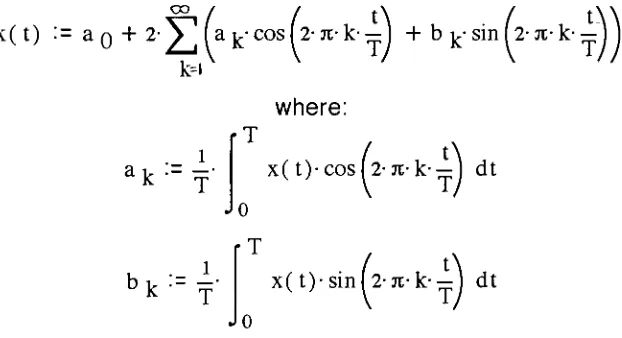
values of Xf.

Given

the

equation

for

discrete

Fourier

transforms:

x(t) :=

ag

+

2-Vj

[a

jc-cos(2-jfk-j

+

b

j,-sin

f

2-%

k-]]

k=i

where:

ak-

x(

t)-cos[2-ji-

k-]

dt

0

bk:=T

x(t)-sin(2-3i-k--J

dt

If

the

continuous

time

series

is

unknown, and

only equally

spaced samples are

known;

we

have

asequence of samples

(xr),

where r=

0,1,2,...

(n-1)

where and

t

=

r*

[image:41.548.122.433.385.554.2]

Replace

the

above

integral

with a summation:

1

^

-i(2,.|).(r.dt)

Xk'=

T

2-.Xr'C

dt

The

Xk

represents

the

wholearea under

the

curve

(See Figure

10).

If T=N*dt is

substituted

then:

A

m

P i -,

i

t

u

d

e

n

G

Sine Wave

x(

t)-cos

xio *"

x:2

0 15 30 45 60 75 90 105120135150165180195 Time

(msec)

Figure

10:

Sine

Wave

used

in DFT

H-l "i-2-jtk-r

Xk:=^

SXre

N

r=o

The

discrete Fourier

transform

(DFT)

of

the

series

{

xr},

r=

0, 1, 2,

...,

(N-1)

is:

Hi)

M-/

Xk:=^X>fe

k-o

withk=0,

1,2, 3,...,

(N-1).

[image:42.548.95.470.163.354.2]

xr

:=X!Xke

Hi)

with r=

0, 1, 2,

3,... (N-1). With

using

the

DFT

method,

the

smaller

the

sampling

interval,

the

closer

the

approximation.

Problems

arise when

trying

to

calculatevalues

for x|<

greater

than

(N-1).

If

k=N+L,

then:

.

i-Xn

+ L:=

N"EXre

2jtl(N+

L)

N

Simplifying,

Xn

+

L:=irZXr

.P

\

N

/.

-i-2-KT

but,

i 1 Jt-r ._

no matter

the

value of

r,

so x_{n+[_}= _{x |_.}

Thus

the

_{coefficientsof x k}

just

_repeat

themselves

for

k>(N-1)

causing

distortion,

which

is

called aliasing.

The Nyquist

frequency

is

defined

as:

At

_=sampling

time

Sampling

Frequency^ _=Sampling

Rate

At

This

is

the

maximum

frequency

that

can

be

detected

from

data

sampled at

time

spacing

dt. The

physical result of

sampling

at a

frequency

too low for

a system

is

that

higher frequencies

are missed

in

measurements.

The

DFT

method of

Fourier transform

was replaced when

J. W.

Cooley

and

J.

W.

Tukey

introduced

the Fast

Fourier

Transform

(FFT)

in

1965.

This

algorithm streamlined

the

computation of

the Fourier Transform

by

changing

the

method used

to

interpolate

constants

in

the trigonometric

polynomial.

This in

combination with

the

integrated

circuit revolution

have

made

frequency

analyzers available

to industry.

The

FFT

equation computes

the

complex

coefficients

Ck

instead

of

ak

and

bk

with

the formula:

2m-₁

F(x)

:=l-Vck-eikx

k=o

where:

jiijk

c^:=yi-em

k

k

for

each

k

=

0, 1,

2

2m

-1.

Time

and

frequency

domains

are

usually

related

through

FFT

and

IFFT

in

the

frequency

analyzers

today

instead

of

DFT

and

I

DFT.

An

outline of

the

process

frequency

analyzers use

for

spectral estimates

is:

1

.

A

discrete time

series

is

created

by

the

results of

sampling the

for

r=

0, 1, 2, 3,...,

(N-1)

_{at a}

time

interval

dt=T/N.

2.

The

Fourier

Transforms for

{Xr}

and

{Yr}

are calculated.

3.

Discrete

series

for

spectral

densities

are

determined from

{Xr}

and

{Yr>.

Appropriate

spectraare

then

derived.

4.

IFFT is

then

used

to

determine

the

corresponding

correlation

functions.

5.3

Error

Classification

There

are

two

classes of error when

dealing

with random

vibration,

bias

error and random error.

Random

error

is

the

result of

the

nature of

the

data,

the

unpredictability

from

one

sampling

to the

next.

The

incident

of random error

is

high

when

sampling is limited.

Bias

errors are consistent errors

in

data

which

are

due

to the

processing

of

the

data

to the

appropriate

format for

the

user.

This

can

be due to

calculation

inefficiencies.

Combined

these

errors pollute

measurements

being

made.

This

is

one reason

why

they

must

be

identified

and

an

understanding

of

how

to

workwith

them

must

be

attained

by

the

user of

spectral analysis and correlation

5.4

Noise

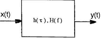
To

understand noise

in

a

system,

use a

ideal

single

input/

single output

x(t)

h(x),H(f)

y(t)

Figure

11:

Ideal Single Input/ Single Output

System

Under ideal

conditions:

y(t)

:= 00

h

(x)

x

(t

-x)

dx

where

h(x)

is

the transfer

function for

the

linear

system

Evaluation

of a system

frequency

response

function

can

be

performed

from

measurement of

x(t)

and

y(t) using

the

equation:

H(f)=

Gxy(f)/Gxx(f)

H(f)

is

acomplex numberwhich can

be

represented

by:

H(f)

=

HR (f)

-

i H

i

(f)

[image:46.548.194.365.27.93.2]

H(f)

:=

|H(f)|-e

i*(f)

|H(f)|

:=

(HR(f)2

₊

H!(f)2)

(|)(f) := atan

:the gain

factor

Hi(0\

HR(f)j

'

:

the

phase

factor

If

the

assumption

is

that

the

input x(t) is

from

a

stationary

random

process,

and

data is

accumulated over sufficient

time

so

that the transients

die

out, the

input/

output auto spectrum relation

is:

Syy(f)

=

I

H(f)

1

2

Sxx

(f)

:

two

sided

Gyy(f)

=

I

H(f)

1 2

Gxx

(f)

:one sided

And the

input/output

cross spectrum relation

is:

SXy(f)

=

H(f) Sxx (f)

:

two

sided

Gyy(f)

=

H(f)

Gxx (f)

:one sided

These

are

true

when

there

is

no extraneous

noise, the

system

is

not

time

varying,

and

there

are no nonlinear characteristics.

n(t)

u(t)

h(T),H(f)

V(t)

^

y(t)

m(Wlux(t)

where:

u(t)

and

v(t)

are

the

true

signals

m(t)

and

n(t)

are noise

terms.

Figure

12:

System

with

Noise

at

Input

and

Output.

Now the terms

x(t)

and

y(t)

consist of:

x(t)

=

u(t)

+

m(t)

and

y(t)

=

v(t) +n(t)

With

noise,

Gum(f)

=

GVn(f)=Gmn(f)=0.

The

system spectral relation

is:

Gw(f)= IH(f)|2

Guu(f)

[image:48.548.163.448.37.146.2]

GUv<f)

=

H(f)

Guu(f).

The

original system spectral

density

functions

are now:

Gxx(f)

=

Guu(f)+Gmm(f)>Guu(f)

Gyy(f)

=

Gvv(f)

₊

Gnn(f)>Gw(f)

Gxy(f)=Guv(f)

The

coherence

is

defined

by

the following:

2._

(|Guv(f)[):

Yuv(f) !=

Gmi(f)-Gvv(f)

uuvw _~vw

-=s

true

coherence

v m*._

QGxy(nD

XV

-("^|f|

is

measured coherence.

In

an

ideal case,

coherence

is

unity.

In

actual

experimentation,

coherence

varies

from

zero

to

one

due

to:

1

.

Noise

in the

measurement.

2.

Bias

errors

in the

spectral estimate.

3.

Nonlinearity

in the

relationship between x(t)

and y(t).

4.

The

output

y(t)

affected

by

inputs

other

than

x(t)

Relating

the two:

IGxy(f)l2=

IGuv(f)l

2

= IH(f)|2 Guu2(f)=

Gw(f)Guu(f)

IH(f)|2

=

Gw(f)/Guu(f)

2

.

Ouu(f)-Gyv(f)

Yxy(0 "=

(Guu(f)+Gmm(f))-(Gvv(f)+Gnn(f))

which

is less

than

or equal

to 1

.

If input

noise exists

in

a

system, then

there

are

two

cases:

1

.

The

noise will pass

through the

system and:

-Hxy(f) will

be

a

biased

estimate of

H(f)

in

gain and phase.

-If

Gxm(f)

is

zero,

Hxy(f)

is

unbiased.

2.

The input

noise

does

not pass

through the

system

then:

- _{gain will}

be

_a

biased

estimate of

H(f),

but

phase will not

be

biased.

- _{phase will}

however

depend

on

the

ratio

Gmm(f)/Guu(f)

known

as

asignal

to

noise ratio.

-GXy(f)

will not

be

influenced,

and

hence

will give a

true

estimate

Guv(f)-If

the

system

has

noise

in

the

output

only (See Figure

13):

n(t)

x(t)

h(T),H(f)

v(t)

"*- y(t)

Figure

13:

System Model

with

Output Noise

only.

For the

model:

input is virtually

noise

free

the

output

is

composed of

v(t)

which

is

due

to

x(t)

and other

deviations

present.

From

the

coherence of

the

noise

in the

system,

eliminating

input

noise,

the

relationships:

Gyy(f)

:=

Gvv(f)

+Gnn(f)

Gvv(f)

:=

Yxy(f) -Gyy(f)

Gnn(f)

:=

(i-Yxy(f)2)-Gyy(f)

Thus

coherence when

there

is

noise at

the

output

is

between

zero and

one,

it

5.5

Frequency

Response

Errors

Estimation

for

frequency

response

in

single

input/

single output systems

involves

both

random and

bias

errors.

It

is extremely

important

that

these

errors

are

understood,

and

if

possible

minimized, for

data

analysis

to

be

credible.

Coherence functions

will aid

in

the

detection

and classification of

errors,

so

it

is

good practice

to

analyze coherence whenever

making

frequency

response

measurements.

5.5.1

Random Errors

in

Frequency

Response

Random

error

in

frequency

response

is

due

to these

common sources:

measurement noise

in

transducers,

computational noise

in data

processing,

other unwanted

inputs,

and

nonlinearity

between

the

input

and

the

output.

Random

error

is

related

to

the

coherence and number of averages used

in

spectral

density

calculation.

To

minimize random error

these

steps should

be

utilized:

1.

Minimize

noise

in instrumentation

by

using

appropriate equipment

(high quality

transducers

when

available,

watch

grounding

loops,

etc.)

2.

If the

coherence

falls

broadly

over a

frequency

range and

the

frequency

response

is relatively

low,

extraneous noise at

the

output

should

be

suspected.

This

can

be

due

to

uncorrelated

inputs

as well.

3.

If

the

coherence

falls

broadly

over a

frequency

range, the

frequency

response

is

not

relatively low

, and

the input

power spectral

Bias

errors could also

be

caused

by

this

scenario.

4.

If the

gain

is sharply

peaked,

as

in

the

case of asystem with slight

damping,

coherence will peak at

corresponding

frequencies.

This

is

due

to

high

signal

to

noise ratios at

these frequencies.

If

the

coherence

does

not peak or even worse

notches, then

n