Rochester Institute of Technology
RIT Scholar Works
Theses Thesis/Dissertation Collections
7-22-2010
Relating Multimodal Imagery Data in 3D
Karl C. Walli
Follow this and additional works at:http://scholarworks.rit.edu/theses
This Dissertation is brought to you for free and open access by the Thesis/Dissertation Collections at RIT Scholar Works. It has been accepted for inclusion in Theses by an authorized administrator of RIT Scholar Works. For more information, please [email protected]. Recommended Citation
Relating Multimodal Imagery Data in 3D
By
Karl C. Walli
B.S., Michigan Technological University, 1991
M.S., Joint Military Intelligence College, 1995
M.S., Rochester Institute of Technology, 2003
A dissertation submitted in partial fulfillment of the
requirements for the degree of Doctor of Philosophy.
Chester F. Carlson Center for Imaging Science
College of Science
Rochester Institute of Technology
July 22, 2010
Signature of the Author ___________________________________________________
CHESTER F. CARLSON CENTER FOR IMAGING SCIENCE
ROCHESTER INSTITUTE OF TECHNOLOGY
ROCHESTER, NEW YORK
CERTIFICATE OF APPROVAL
Ph.D. DEGREE DISSERTATION
The Ph.D. Degree Dissertation of Karl C. Walli has been examined and approved
by the dissertation committee as satisfactory for the dissertation
required for the Ph.D. Degree in Imaging Science
Dissertation Advisor: _______________________________________
Dr. John Schott
Committee Member: _______________________________________
Dr. Harvey Rhody
Committee Member: _______________________________________
Dr. Carl Salvaggio
External Chair: _______________________________________
v
DISSERTATION RELEASE PERMISSION
CHESTER F. CARLSON CENTER FOR IMAGING SCIENCE ROCHESTER INSTITUTE OF TECHNOLOGY
Title of Dissertation:
Relating Multimodal Imagery Data in 3D
I, Karl C. Walli, hereby grant permission to Wallace Memorial Library of R.I.T. to reproduce my dissertation in whole or in part. Any reproduction will not be for commercial use or profit.
vii
Disclaimer
The views expressed in this dissertation are those of the author and do not reflect the official policy or position of the United States Air Force, Department of Defense, or the
ix
Relating Multimodal Imagery Data in 3D
By
Karl C. Walli
Chester F. Carlson Center for Imaging Science
College of Science
Rochester Institute of Technology
ABSTRACT
This research develops and improves the fundamental mathematical approaches and
techniques required to relate imagery and imagery derived multimodal products in 3D. Image
registration, in a 2D sense, will always be limited by the 3D effects of viewing geometry on the
target. Therefore, effects such as occlusion, parallax, shadowing, and terrain/building elevation
can often be mitigated with even a modest amounts of 3D target modeling. Additionally, the
imaged scene may appear radically different based on the sensed modality of interest; this is
evident from the differences in visible, infrared, polarimetric, and radar imagery of the same
site.
This thesis develops a ‘model-centric’ approach to relating multimodal imagery in a 3D
environment. By correctly modeling a site of interest, both geometrically and physically, it is
possible to remove/mitigate some of the most difficult challenges associated with multimodal
image registration. In order to accomplish this feat, the mathematical framework necessary to
x
to be generated to apply this ‘model-centric’ approach, this research develops methods to
derive 3D models from imagery and LIDAR data. Of critical note, is the implementation of
complimentary techniques for relating multimodal imagery that utilize the geometric model in
concert with physics based modeling to simulate scene appearance under diverse imaging
scenarios. Finally, the often neglected final phase of mapping localized image registration
results back to the world coordinate system model for final data archival are addressed.
In short, once a target site is properly modeled, both geometrically and physically, it is possible
to orient the 3D model to the same viewing perspective as a captured image to enable proper
registration. If done accurately, the synthetic model’s physical appearance can simulate the
imaged modality of interest while simultaneously removing the 3-D ambiguity between the
model and the captured image. Once registered, the captured image can then be archived as a
texture map on the geometric site model. In this way, the 3D information that was lost when
the image was acquired can be regained and properly related with other datasets for data
xi
Table of Contents
Page
1 Introduction ... 1-1 1.1 Use of Imagery Data is now Mainstream ... 1-1 1.2 The Problem ... 1-2 1.3 The Solution ... 1-3 1.4 The Advanced ANalyst Exploitation Environment (AANEE) ... 1-5 1.5 The 3D Model as an Archival Database ... 1-7 1.6 Summary ... 1-8
2 Image Registration ... 2-1 2.1 Invariant Feature Extraction ... 2-2 2.1.1 Laplacian of Gaussian (LoG) Filter ... 2-2 2.1.2 Difference of Gaussian Filter ... 2-6 2.2 Matching Invariant Features ... 2-8 2.2.1 Point Matching using Distance Similarity ... 2-9 2.2.2 Point Matching using Localized Gradient Similarity ... 2-12 2.3 Transform Development ... 2-16 2.4 Constraining the Transform Results – 2D Conformal and Affine ... 2-20 2.5 Outlier Removal and Error Analysis ... 2-21 2.5.1 RMSDE Analysis ... 2-22 2.5.2 Random Sample Consensus (RANSAC) Analysis ... 2-23
xii
3.2.3 Case Study - Estimating Model Pose from unknown Imagery ... 3-17 3.3 SWIR Imagery to SWIR Attributed LIDAR Models ... 3-19
4 Deriving Sparse Structure from Images ... 4-1 4.1 Feature Extraction and Matching ... 4-3 4.2 Modern Photogrammetric Techniques ... 4-5 4.2.1 Approach – Depth Recovery from Overlapping Images ... 4-6 4.3 Case Study – Creating Sparse Structure using Airborne Data ... 4-14 4.3.1 AeroSynth Introduction ... 4-14 4.3.2 Recovering Sparse Structure from Images ... 4-15 4.3.3 Recovering Dense Structure from Images ... 4-28 4.3.4 AeroSynth Summary ... 4-33 4.4 Sparse Bundle Adjustment (SBA) ... 4-34
5 Relating Rigid 3D Bodies ... 5-1 5.1 Sparse to Dense Point Clouds ... 5-2 5.1.2 Approach ... 5-4 5.1.3 Case Study ... 5-5 5.2 Point Cloud to Faceted Model (FM) ... 5-8 5.2.1 Approach ... 5-9 5.2.2 Case Study ... 5-9 5.3 Future Research ... 5-11 5.4 Faceted Model to Faceted Model ... 5-14 5.4.3 Approach ... 5-14 5.4.4 Case Study ... 5-15 5.5 Constraining the Transform – 3D Conformal and Affine ... 5-17 5.5.1 Conformal 3D Transform ... 5-18 5.5.2 Affine 3D Transform ... 5-22 5.5.3 Homogeneous 15 Parameter Linear Estimate ... 5-24 5.5.4 Nonlinear Minimization and Weighting... 5-25
xiii
6.2.3 LIDAR Direct – Developing LIDAR models in DIRSIG ... 6-16 6.2.4 Imagery Direct - Developing Multiview Imagery models in DIRSIG ... 6-21 6.3 Simulate – Physically (DIRSIG) ... 6-24 6.3.1 Simulating WASP Imagery with DIRSIG ... 6-26 6.3.2 Simulating Materials and their associated Emissivity Curves in DIRSIG ... 6-27 6.3.3 Example DIRSIG Simulations of the Hybrid Model ... 6-31 6.3.4 Example DIRSIG Simulations of the LIDAR Direct Model ... 6-35 6.4 Relate - Mathematically ... 6-37 6.4.1 Error Analysis ... 6-39 6.4.2 Image Registration to the Hybrid DIRSIG Model ... 6-42 6.4.3 Image Registration to the LIDAR Direct DIRSIG Model ... 6-48 6.4.4 Reorient the Model to Incorporate the Registration Results ... 6-51 6.5 Archive – Texturally (Map the Real Image to the Model) ... 6-53 6.5.1 Model Pose from Matched Features ... 6-53 6.5.2 Projective Texture – Image to Model ... 6-54 6.6 Results Summary – DIRSIG as a Multimodal Rosetta Stone ... 6-60
7 Relating Results in the World Coordinate System ... 7-1
8 Research Contributions ... 8-1 8.1 Photogrammetric and Epipolar Geometry based Terrain Recovery ... 8-1 8.2 Constrained Conformal and Affine 3D Transformation ... 8-2 8.3 DIRSIG 3D Multimodal Registration ... 8-2 8.4 Comprehensive Breadth – Multi-Dimensional/Modal Research ... 8-3 8.5 Suite of MATLAB Software Tools ... 8-3
9 Summary ... 9-1
10 References... 10-1
11 APPENDIX A - Camera Calibration ... 11-1 11.1 The Camera External Orientation Parameters (EOPs) ... 11-1 11.2 The Camera Interior Orientation Parameters (IOPs) ... 11-2 11.3 Radial Lens Distortion Parameters ... 11-3
12 APPENDIX B - Linear Estimation ... 12-1 12.1 The Projection Matrix Revisited ... 12-1 12.2 The Direct Linear Transform (DLT) ... 12-2
xiv
13.1 The Levenberg-Marquardt Algorithm ... 13-1
14 APPENDIX D - Epipolar Techniques for Recovering Sparse Models ... 14-1 14.1 Approach ... 14-1 14.2 Develop a Linear Estimate of the Camera Parameters ... 14-2 14.3 Develop a Linear Estimate of the 3D Points ... 14-3 14.4 The Essential Matrix ... 14-6 14.5 Case Study – Creating Sparse Structure using Epipolar Geometry ... 14-10
15 APPENDIX E - Model Texture ... 15-1 15.1 Image Draping ... 15-2 15.2 Facet Texturing and Model Unwrapping ... 15-3 15.3 Projective Texturing ... 15-5 15.4 Volumetric Pixel (Voxel) Texturing ... 15-5
16 APPENDIX F – DIRSIG Simulation Setup Primer ... 16-1 16.1 DIRSIG’s Scene File Setup ... 16-1 16.2 DIRSIG’s Sensor File Setup... 16-5 16.3 DIRSIG’s Platform File Setup ... 16-8 16.4 DIRSIG’s Atmospheric Conditions Setup ... 16-11 16.5 DIRSIG’s Data Collection Setup ... 16-11
xv
List of Figures
Page
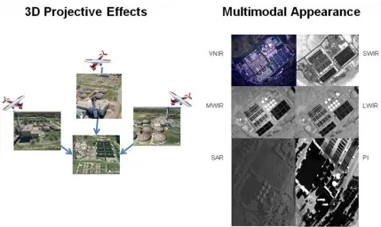
Figure 1-1 – This Google Earth (Google Earth 2010) view of the VanLare Site contains a hi-fidelity model courtesy Pictometry Int. (Pictometry 2010) and is representative of the realistic representations possible within today’s GIS environments. ... 1-1
Figure 1-2 The registration challenges resulting from viewing geometry including parallax, occlusion, & shadowing (left) and spectral diversity (right) are visible above (synthetic SAR and PI images of VanLare courtesy Dr Mike Gartley). ... 1-3
Figure 1-3 This graphic shows the result of registering two images of San Diego, where ~75% of the correctly matched features (red squares) were discarded in a vain attempt to obtain subpixel registration accuracy to a 2D model. ... 1-4
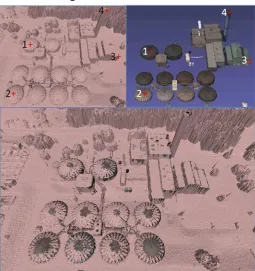
Figure 1-4 – The scenes above show the same model of the VanLare Plant from within the AANEE software program. Note the accurate casting of shadows and the ability to predict occlusions due to the 3D modeled site and landscape. ... 1-6
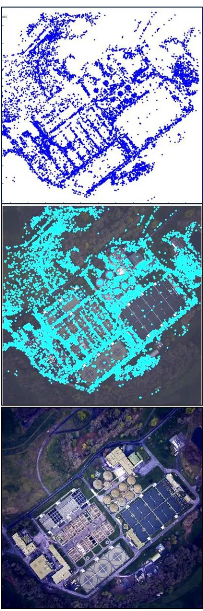
Figure 1-5 - This view of the VanLare site from the AANEE software program contains
projections of additional RGB and LWIR data from RIT’s WASP sensor over the site and terrain model, before registration; using only sensor IMU/GPS data. ... 1-7
Figure 1-6 The five primary areas of research contained in this dissertation are covered in Chapters 2-6. ... 1-9
Figure 2-1 The basic process for automatically relating images. ... 2-1
Figure 2-2 Demonstration of the LoG filter effects on synthetic edge data... 2-3
Figure 2-3 Edge-exaggeration resulting from convolution with a 1D LoG filter ... 2-3
Figure 2-4 Visual effect of the Laplacian of Gaussian Filters in succession. ... 2-5
Figure 2-5 A 1-D representation of the LoG function and the composite 5x5 approximated filter. ... 2-5
Figure 2-6 The results of the LoG filter and thresholding of maxima to create Control Points. 2-6
Figure 2-7 The 1D visualization of the inverted DoG as the result of subtracting two Gaussian kernels of different widths (Drakos and Moore 2007). The inset graphic shows little if any perceivable difference between the LoG and DoG convolution kernels (Gonzalez and Woods 2007). ... 2-7
Figure 2-8 Matching points to determine the Image Transform. ... 2-8
xvi
Figure 2-10 Each set of points has the same cross ratio and are related via line-to-line
projectivity ... 2-11
Figure 2-11 For every octave of scale space the initial image is convolved with Gaussians of varying standard deviations and subtracted from their neighbors producing a DoG pyramid ... 2-12
Figure 2-12 Maxima and Minima of the DoG pyramid stacks are detected by comparing each pixel with its 26 neighbors in 3x3 regions at the current and adjacent scales (D. G. Lowe 2004). ... 2-13
Figure 2-13 Keypoint descriptors are created by computing the gradient magnitude and
orientation, Gaussian weighted by the pixels location, surrounding a keypoint. These samples are then accumulated into 8 bin orientation histograms, which summarize a 4x4 subregion (D. G. Lowe 2004). ... 2-14
Figure 2-14 Thousands of invariant keypoints generated and matched using the SIFT algorithm. ... 2-15
Figure 2-15 Utilizing RMSDE as a Metric to cull Outliers; note the distinctive “knee” in the error curve. ... 2-23
Figure 2-16 A) A dataset with outliers; B) Shows how a line can be determined with the minimal number of two points and how the inliers are tallied; C) Shows how two close points can provide poor extrapolation and low inlier count; D) Shows the “correct” solution for culling the outliers. ... 2-24
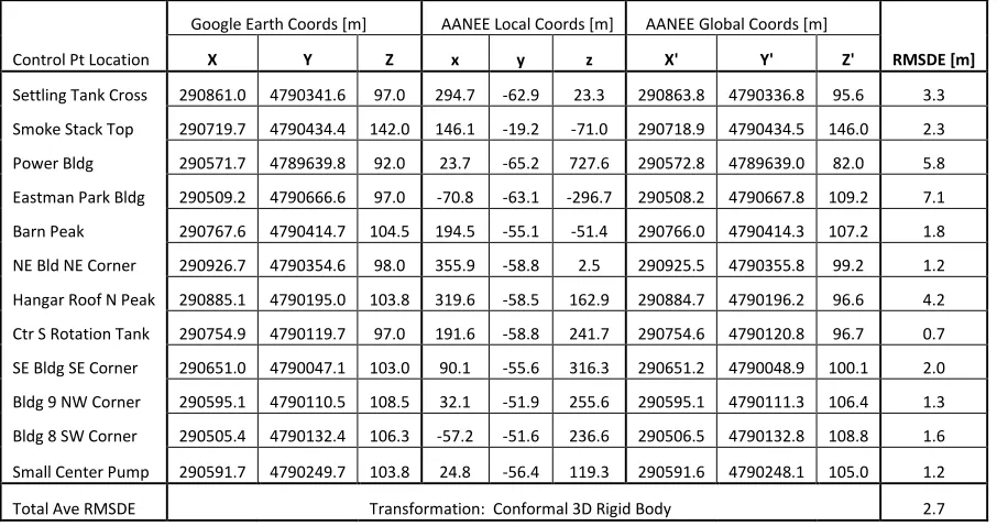
Figure 3-1 In this Pseudo-Color composite of the WASP SWIR/MWIR/LWIR composed as an RGB image stack, the Northern Bldg at the VanLare Plant (Red Circle) was recently built and is evidently made of a different material than its neighbors. ... 3-2
Figure 3-2 The process for relating an image to a model when the camera pose is known starts with changing the orientation of the model to mimic the known sensor view. Then the extraction and matching of similar features from the image and model can occur in similar 2D construct. These matches are then used to refine the model pose (due to IMU/GPS precision error) for final projective texturing of the image on the model. ... 3-3
Figure 3-3 Even rudimentary models textured with images (top) can be used to simulate the 3D effects of scene projection, shadowing, and occlusion evident within real images (bottom) and can thus allow for precise 2D registration. ... 3-4
Figure 3-4 The general process utilized to register images to GIS modeled scenes. ... 3-5
Figure 3-5 The top image with initial IMU/GPS pose and the bottom after affine correction. Both images are displayed in Google Earth with 30m accuracy terrain and detailed Pictometry model of the VanLare Site. ... 3-7
xvii
Figure 3-7 The basic process for relating images to a model when the camera pose is unknown. The main difference here is that the initial camera pose must be solved for using correspondences or user manipulation of the model pose. At this point the process then mimics the one described earlier in Section 3.1. ... 3-10 Figure 3-8 Algorithm 7.1 – The Gold Standard Algorithm for estimating P from world to image
point correspondences in the case that the world points are very accurately known. 3-11
Figure 3-9 This simple graphic displays how a linear estimate of a nonlinear function can provide a rough estimate of the local/global minimum location, within some margin of error. ... 3-15
Figure 3-10 On the left is the working image with the same 12 locations selected as on the model; these locations are twice the number required for resectioning with a model (6 GCPs). ... 3-17
Figure 3-11 On the left, the DLT provides a good starting point for LMA to optimize a solution. ... 3-18
Figure 3-12 The figure above show a 2D SWIR image (A) and an image projection of a 3D model that was textured/attributed using the same LIDAR SWIR intensity returns that were utilized to create the facetized 3D model. ... 3-19
Figure 3-13 The results of automated registration (using SIFT & RANSAC), between the 2D SWIR image and the 3D LIDAR model are apparent. ... 3-20
Figure 4-1 This graphic depicts the six basic steps required for relating multiple images to recover sparse structure via the Bundle Adjustment process. Once invariant features are extracted and matched, a linear estimate of the 3D point set is fed into a Bundle Adjustment process to simultaneously optimize the model points and camera
parameters. ... 4-2
Figure 4-2 The epipolar relationships of the cameras, image points, and model points. ... 4-4
Figure 4-3 Hartley & Zisserman’s 7-Point Fundamental Matrix using RANSAC. ... 4-5
Figure 4-4 Process for tiling images larger than 2kx2k for SIFT feature extraction and matching. ... 4-7
Figure 5 Displays the utility of RANSAC plane fitting to SPC terrain data for outlier removal.. 4-8
Figure 4-6 Rectification of the matches must be performed for accurate 3D estimation of the SPC. ... 4-9
xviii
Figure 4-8 The overlapping images above (red & yellow) are registered and have matches that are common to all (cyan). These common locations can then be utilized for 3D
registration or as seeds for the DPC extraction process (Section 4.3.3). ... 4-11
Figure 4-9 Once the image bundle is optimized using SBA, it is possible to relate the images, cameras and 3D point cloud into a 3D mathematical framework to determine the region of overlap for DPC interrogation and additional processing. ... 4-12
Figure 4-10 The basic process for developing Dense Point Clouds using Epipolar relationships between images. ... 4-13
Figure 4-11 Example showing the angular diversity required to recover 3D Terrain from
Airborne Imagery. ... 4-15
Figure 4-12 Thousands of invariant keypoints generated and matched using the SIFT algorithm. ... 4-17
Figure 4-13 Depiction of the Fundamental Matrix constraint between images which is used for outlier removal. ... 4-18
Figure 4-14 Graphic showing two collection stations of an airborne sensor utilized to recover 3D Structure. ... 4-20
Figure 4-15 Corrections are required to compensate for aircraft pitch, yaw, and roll and flight line orientation as discussed earlier in Section 4.2.1.3. These are done by projecting the matches onto a virtual focal plane and then transforming them to a coordinate system aligning the x-axis to the flight line connecting the two image centers. ... 4-21
Figure 4-16 The interim estimates of the four individual SPC’s can be seen compared to the camera locations. ... 4-23
Figure 4-17 Example results of the Sparse Bundle Adjustment process on the Sparse Point Cloud. Here the absolute global coordinates (A) can be compared to the facetized surface (B), visualized in Google Earth (C), or re-projected back into any of the images contained within the bundle (D). ... 4-26
Figure 4-18 The image derived SPC mesh fidelity can be directly compared to both hi-fidelity ~1 [m] LIDAR terrain and a lo-fidelity ~30 [m] Digital Elevation Map. ... 4-27
Figure 4-19 Left: Image with single point chosen. Middle/Right: Corresponding epipolar lines in other images. ... 4-29
Figure 4-20 Left: Initial estimate of the structure of the dense point cloud from three images. Right: Result after SBA, world coordinate mapping and projective image texturing. .. 4-30
xix
Figure 4-22 Matching between a nadir and oblique images using ASIFT and then RANSAC with the Fundamental Matrix as the fitting model (Images courtesy Pictometry Int.
(Pictometry 2010)). ... 4-32
Figure 4-23 Growing 3D depth maps based on the initial SPC results and epipolar relationships. In the upper left inset, the 3D SPC is projected back onto the base image. For these locations the depth information is already known (upper right) and can be used to constrain the matching locations in the other images (lower left) to follow a general surface function. ... 4-33
Figure 4-24 The structure and composition of a Bundle Adjustment Jacobian matrix. ... 4-35
Figure 4-25 The structure and composition of the normal equations (~Hessian matrix). ... 4-35
Figure 4-26 A sparse matrix obtained when solving a modestly sized bundle adjustment
problem. This sparsity pattern is of a 992x992 normal equation (i.e. approx. Hessian) matrix, where black regions are nonzero blocks. (Lourakis and Argyros 2009) ... 4-36
Figure 5-1 The basic process for relating 3D models and structure using a 3d Conformal transform. As in the previous sections, the key here is to relate similar features within the two datasets in order develop a mathematical relationship. The only added complexity is in the additional dimensionality and possible feature disparity of the datasets. ... 5-2
Figure 5-2 The Midland Site SPC (top) resulting from BA of tens of thousands of 3D points compared to the millions of 3D points embedded within a LIDAR DPC (Bottom). .... 5-3
Figure 5-3 Relating the SPC pts to DPC points via an iterative nearest neighbor approach. ... 5-5
Figure 5-4 The image derived SPC mesh above is compared to a LIDAR derived DPC mesh below for comparison in Meshlab. The absolute coordinates of the image derived results are only as accurate as the projected location of the base image, so a final
translation, acquired from the matched locations (right), may be necessary. ... 5-7
Figure 5-5 The results of the linear 3D Translation and Meshlab (Pisa 2010) implemented ICP nonlinear refinement can be visualized above. Note the general agreement between LIDAR and SPC surfaces as they fight for visibility across the scene. ... 5-8
Figure 5-6 This illustrations shows the initial LIDAR DPC with grayscale intensity attributed points on the left. This can be utilized to produce a clean facetized model utilizing the author’s MATLAB code as shown in the graphic on the right. ... 5-9
Figure 5-7 This graphic portrays a manual feature correspondence generation that can be used to relate a Faceted Model to a LIDAR DPC that has been facetized. Once
accomplished, the initial relationship is improved through nonlinear ICP analysis. 5-10
xx
Figure 5-9 The Bundle Adjusted VanLare Site SPC (top), was projected back into the base image (Middle) and can then be compared directly with the FM where the base image is used as a UV texture on the terrain (Bottom). ... 5-13
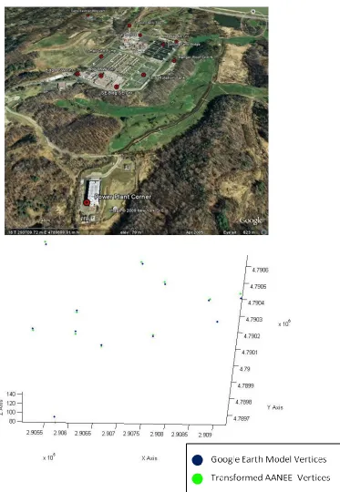
Figure 5-10 The Control Points used to related the GE and AANEE models (top) and the resulting transformation of the local points into Global UTM coordinates when
compared to their matching Google Earth locations (bottom). ... 5-16
Figure 6-1 Multimodal image synthesis using DIRSIG’s physics based modeling *courtesy Dr. Mike Gartley ... 6-1
Figure 6-2 Multimodal imagery registered to GE textured terrain using user assisted GCP selection and overlaid upon the initial sensor derived (IMU/GPS) global coordinate predictions. The inverted contrast of water in VNIR and Infrared is circled. ... 6-2
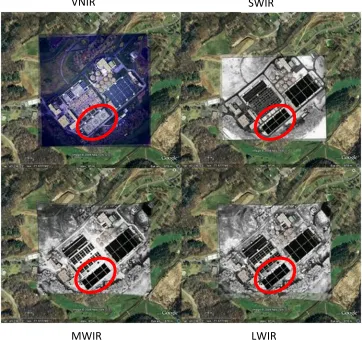
Figure 6-3 This figure illustrates the MSRA Approach to 3D Multimodal Registration, where A) is the modeling phase, B) is the physics based simulation phase, C) is the 2D image registration phase, and D) is the Image archival phase onto a model. ... 6-4
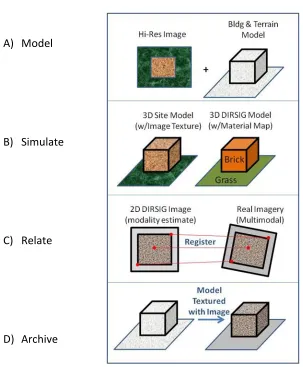
Figure 6-4 This flowchart illustrates three different paths for generating geometric models for DIRSIG simulation. From left-to-right they are Existing/User Created, LIDAR Derived, and Multiview Image Derived models with varying degrees of fidelity. ... 6-5
Figure 6-5 This Hi-Fidelity model of the VanLare Waste Water Processing plant is representative of an existing geometric model placed in Google Earth that utilizes UV mapped image textures for added realism (courtesy Pictometry Int.) ... 6-6
Figure 6-6 This illustration depicts the process of adding spectral reflectance curves to a realistic scene model in DIRSIG using Hyperspectral or Advanced Spectrometer Data (ASD) to properly simulate material appearance in various spectra. ... 6-7
Figure 6-7 Illustrates the UV Texturing process: A) The wireframe model, B) The faceted model, C) The UV textured Model, D) The flattened (unwrapped) model with overlaying image texture, and E) The textured wireframe model. ... 6-8
Figure 6-8 This graphic illustrates the process used to turn a UV Texture map (A), into a material class map LUT (C) by first segmenting the image with a K-Means classifier (B). ... 6-9
Figure 6-9 This flowchart depicts the process utilized for DIRSIG model creation using hybrid models and imagery. ... 6-11
Figure 6-10 This figure illustrates the process utilized to register a site model (A), to a faceted LIDAR dataset (B), to assess model fidelity and to ensure proper building placement and dimensions (C). Finally the model is placed on the bare earth LIDAR terrain (D) to create a hybrid scene using both the LIDAR terrain and Image derived building
models. ... 6-13
xxi
Figure 6-12 The process by which a LIDAR Return Point Cloud (A), can be transformed into model facets textured with real imagery of the forested terrain (B). The results of this process can be viewed above in MATLAB (C) or Meshlab (D). ... 6-15
Figure 6-13 The final model of the VanLare site, as viewed in Blender, using manually derived multiview imagery building models (courtesy Pictometry Int.) and LIDAR derived terrain and tree models. ... 6-16
Figure 6-14 This flowchart depicts the process utilized for DIRSIG model creation using LIDAR data and imagery. ... 6-17
Figure 6-15 This graphics shows the 3 stages in transforming LIDAR data from a Point Cloud (A), to a faceted model (B), and finally texturing that model with the intensity return of the LIDAR itself (C). ... 6-18
Figure 6-16 The LIDAR Direct process involves utilizing Imagery (A), to create a material map in order to physically describe the site. Here, automated segmentation of the terrain (B) is used in concert with user assisted ID of site materials (C). ... 6-19
Figure 6-17 By using the spatial, brightness, and facetized characteristics of the LIDAR returns, aggregate material identification for DIRSIG should be possible. ... 6-20
Figure 6-18 The relative quality of terrain information as derived from LIDAR, Multiview
Imagery, and RADAR respectively. ... 6-22
Figure 6-19 The ability to use Multiview Imagery derived Surface Elevation Maps to
orthorectify an image is shown above. ... 6-23
Figure 6-20 The physics based simulation process that DIRSIG utilizes for synthetic image generation (Digital Imaging and Remote Sensing Laboratory 2006). ... 6-26
Figure 6-21 The general process involved when associating emissivity curves to intensity values from an image texture map. Here a region of interest was extract from the image and compared to the 44 curve emissivity plot (bottom) and the DC Histogram (right). Ideally, a simulation could link every DC value to a specific emissivity curve (i.e. 256 curves needed here). ... 6-28
Figure 6-22 When only one emissivity curve exists in the material file, all of the image texture intensity values will be associated with only the singular curve. This will result in no texture information “coming through” in the DIRSIG simulation. ... 6-29
Figure 6-23 The resulting emissivity expansion of the original gravel roof material from 44 curves to 400. ... 6-30
Figure 6-24 The simulated DIRSIG images above illustrate the need for material files with numerous emissivity curves to allow proper reconstruction of image texture within a scene. ... 6-31
xxii
buildings, but, the tree facets are reduced in size due to the cosine viewing effect. .. 6-32
Figure 6-26 In the figure above, the Southern (left) and Northern (right) sections of the VanLare plant are again visible at an oblique angle, but, now in slightly greater detail. ... 6-32 Figure 6-27 On the left is a contrast enhanced image of the VanLare plant taken by the WASP
imaging system, while on the right, is similarly enhanced DIRSIG simulation of the same site using the WASP view and the Hybrid model of the site. ... 6-33
Figure 6-28 The Northern portion of the VanLare Plant around the Smokestack and storage vats, imaged by WASP (left) and simulated by DIRSIG (right). ... 6-33
Figure 6-29 The Southern portion of the VanLare Plant around the administration buildings, imaged by WASP (left) and simulated by DIRSIG (right). ... 6-34
Figure 6-30 On the left is an image of the VanLare plant taken by the WASP SWIR sensor, while on the right, is a DIRSIG simulation of the site, in the same spectral region, using the WASP view and the Hybrid model of the site. ... 6-35
Figure 6-31 The LIDAR Direct process involves utilizing Imagery Textures and Materials Maps (A), with user assisted identification of dominant site materials (B) for ingestions into DIRSIG to physically simulate the site (C). ... 6-36
Figure 6-32 The LIDAR Direct DIRSIG simulation’s similarity to real imagery is readily apparent. The ability to relate LIDAR derived models, textured with archival imagery, to newly acquired images is key to the model centric approach. ... 6-36
Figure 6-33 DIRSIG simulated image in the SWIR region (A) compared to an actual image from the WASP sensor acquired in the same SWIR region and from a similar camera position and orientation. ... 6-37
Figure 6-34 The basic process for relating multimodal image bundles utilizing DIRSIG. Here the model show various “colored” cubes that represent the 3D physical model which can be projected into an image of various modalities. ... 6-38
Figure 6-35 The images above show the initial WASP SWIR image paired with its DIRSIG
simulation and the initial features matched using SIFT (A), the outliers removed using RANSAC with the F-Matrix (B), which were supported by using RANSAC with the M-Matrix (C), and finally where the largest contributing error match was removed using RMSDE analysis. ... 6-45
Figure 6-36 In the left plot, the initial RMSDE is plotted w.r.t. the number of good matches. After the largest error contributor was removed, the data was used to create a new model with error distributed slightly more linearly. ... 6-47
Figure 6-37 The results of the transformed DIRSIG simulated image (right), when compared to the WASP SWIR image (left)... 6-47
xxiii
Figure 6-39 The Sequence above illustrates the features extracted using SIFT (A), outlier removal using RANSAC (B), and the final transformation using the resulting good matches (C), which resulted in sub-pixel registration accuracy. ... 6-50
Figure 6-40 By ray tracing from the camera to the simulated image correspondence location it is possible to isolate the 3D model location of interest for use in pose estimation. 6-54
Figure 6-41 To obtain “vertex texture” locations for UV mapping a model to an image starts at the camera and then projects the 3D model onto a 2D image. The projected model vertex locations on the image are the texture locations. ... 6-55
Figure 6-42 This series of snapshots show how the matches from the base image can be directly related to the 3D SPC model and then used as the vertex texture locations with the base image to create the model’s UV Texture map. ... 6-57
Figure 6-43 This figure shows the IR Attributed LIDAR model from a NADIR (right) and an
oblique (left) view. ... 6-59
Figure 6-44 A summary of the DIRSIG Rosetta Stone strengths regarding multimodal image registration. ... 6-61
Figure 7-1 Relating the cameras, images, and structure to a World Coordinate System augments the mathematical relationships developed in Chapter 4, by combining it with the 3D Conformal techniques of Chapter 5 within a GIS construct. ... 7-2
Figure 7-2 The relationships between the 2D/3D Homographies (H), Projection Matrix (P), and Colinearity Equations. ... 7-4
Figure 14-1 The Essential Matrix relates the two images using a simple 3D translation and rotation of the cameras. ... 14-8
Figure 14-2 The graphics above show the results of Microsoft’s PhotoSynth BA process. ... 14-11
Figure 14-3 The SPC (top) and resulting mesh (bottom) from the Bundler SBA process (Snavely, Bundler 2010) using VNIR images from the WASP sensor. ... 14-12
Figure 15-1 An illustrative example of IR image fusion in the form of a pseudo-color image stack. Circled in red is a new building that was constructed from different material (green metal) than the surrounding brick buildings with gravel roofs. ... 15-1
Figure 15-2 By using a model (left) and related image (middle) it is possible to produce a realistic scene (right), as visualized using one of the demonstration tutorials within the IDL programming environment (ITT Visual Information Solutions 2008). ... 15-2
Figure 15-3 These multimodal models have been textured with image segments on each facet (visible-left & thermal-right). ... 15-3
xxiv
Figure 15-5 Illustrates the UV Texturing process: A) The wireframe model, B) The faceted model, C) The UV textured Model, D) The flattened (uwrapped) model with
overlaying image texture, and E) The textured wireframe model. ... 15-4
Figure 15-6 Here the same model has been textured using a projection tool in Sketchup (Google Sketchup 2009) and then imported into Google Earth (Google Earth 2010). ... 15-5
Figure 15-7 Volumetric Pixel (Voxel) approach to save data in volumetric space, but attribute as 2D facet. ... 15-6
Figure 16-1 The DIRSIG Simulator Editor provides access to various components of the
program. ... 16-1
Figure 16-2 The Geometry tab (A), in the DIRSIG Scene editor, references the model geospatial and directory location, while the Material tab (B) links to the scene materials
description file and emissivity file directory. ... 16-2
Figure 16-3 Within the Scene “Property Map” tab there are links (left panel) to the Material Map descriptions for the site (C) and Texture Maps (D). These “Property Maps” are tightly coupled within DIRSIG for physical scene description. ... 16-3
Figure 16-4 The Sensor Editor has links to a Mount Editor (A) and the Imaging Camera in the Left Panel. As seen here, the Mount interface was utilized to capture the sensor viewing angles which were retrieved from an Inertial Measurement Unit. ... 16-5
Figure 16-5 Within the Camera Instrument editor, there is an “edit” button for the Focal Plane (B). Pressing this button will bring up the Focal Plan Edit menu with additional
buttons for editing the Detector Array (C) and the Response Curve (D)... 16-6
Figure 16-6 The Focal Plane editor buttons bring up the Detector Array editor (C) and Detector Spectral Response editor (D) windows, which allow a great deal of flexibility in
defining the sensor specific design characteristics. ... 16-7
Figure 16-7 The Platform Editor allows for the designation of geospatial position information, such as Latitude, Longitude, Altitude and the orientation information of the sensors External Orientation Parameters, such as Pitch, Yaw & Roll. ... 16-8
Figure 16-8 In order to properly inject the WASP GPS/IMU data into DIRSIG it is essential to convert for any local coordinate translations, sensor angles and Geoid offsets. For the VanLare site, this offset accounts for 36 [m] higher flying altitude. ... 16-9
Figure 16-9 DIRSIG’s 5 MegaScene Tiles (courtesy Mike Presnar) cover a swath of Northern Rochester and include a variety of environmental settings, including residential, agricultural, industrial, and lake frontage. The VanLare test site is in Tile-4. ... 16-10
xxv
Figure 16-11 The Data Collection Editor allows the user to designate the day and time of collection; this is essential for properly casting shadows onto the scene from the correct solar position. ... 16-12
Figure 17-1 This flowchart provides a snapshot of the tools provided for image registration and the related file structure ... 17-1
Figure 17-2 This flowchart provides a snapshot of the tools provided for SPC Generation and the related file structure ... 17-2
Figure 17-3 This flowchart provides a snapshot of the tools provided for Pose Estimation and the related file structure ... 17-3
Figure 17-4 This flowchart provides a snapshot of the tools provided for Model Registration and the related file structure. ... 17-3
xxvii
Glossary
Bundle Adjustment. A photogrammetric process utilized to relate multiple cameras, images and the resulting sparse structure by solving for the camera’s external and internal parameters w.r.t. corresponding image control points.
Dense Point Cloud (DPC). An array of 3D points, that is often associated with a LIDAR dataset and is described by a global coordinate system.
Discrete Linear Transform (DLT). A linear technique that can provide an initial estimate of a solution space that is often desired to seed a non-linear optimization algorithm.
Exterior Orientation Parameters (EOP). These parameters refer to the location of the camera lens *X, Y, Z+ and the orientation of the camera *ω, φ, κ+ at the time of image capture.
Faceted Models (FM). This refers to the traditional computer graphics models that contain vertices and facets to represent the 3D structure of a scene.
Interior Orientation Parameters (IOP). These parameters refer to the intrinsic properties of the camera and include focal length, principle point, focal plane skew, and radial distortion.
Levenberg-Marquardt Algorithm (LMA). A robust nonlinear optimization technique often used in computer vision problems for estimating the solution to nonlinear least squares problems.
Random Sample Consensus (RANSAC). A technique for robustly removing outliers from a dataset. It does this by minimally sampling the data a statistically significant number of times to create a mathematical model that maximizes the number of inliers within an error region.
Space Resectioning. A photogrammetry term that implies solving for a camera’s pose by relating points in one image to those in another, or to a model.
Sparse Bundle Adjustment (SBA). The term “sparse” here relates to the sparse matrix techniques utilized to solve for extremely large, but, weakly correlated parameters involved when solving for most Bundle Adjustments.
Sparse Point Cloud (SPC). The array of 3D points locally defined within a 3D coordinate system.
Sparse Structure Bundle (SSB). This includes the entire bundle of sparse structure, images and related camera positions within a common and local 3D coordinate system.
UV Texture Map. A standard technique in the graphic modeling community used to realistically texture 3D models. This technique maps a composite texture, mapped in the normalized
‘ , to the vertices of select model facets; thus obtaining the name “UV Texture Map”.
1-1
1
Introduction
1.1 Use of Imagery Data is now Mainstream
Over the course of the last decade, the use of imagery based products from airborne and
satellite platforms have become mainstream. Applications like Google Earth/Maps (Google
Earth 2010) and Bing Maps (Microsoft Corporation 2010) allows a user to plan travel, assess
real-estate, teach their children geography, or visualize where the latest ‘crisis du jour’ is
happening in the world at the click of a mouse button. The ability to seamlessly view hundreds
of integrated image products in visual databases has thrown open the doors on the once “niche
field” of imagery analysis, integration, fusion, and database archival.
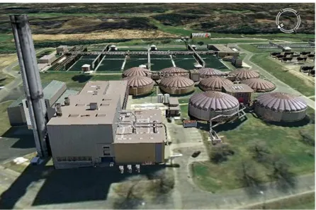
[image:30.612.127.486.395.660.2]The VanLare Water Processing Plant – Google Earth Software View
1-2
Along with this keen new interest by the general population in seeing a “bird’s eye view” of the
world, comes new mathematical advancements from the field of computer vision that are
allowing robots to perceive their surroundings and avoid obstacles. What do these two
observations have in common? They both require the processing of large volumes of imagery
that are captured from a multitude of vantage points, registered together, and provided in local
or global 3D coordinate systems that allow for integration, fusion and archival.
1.2 The Problem
Although great strides have been made in the automated registration of grayscale imagery from
similar viewing geometries, there are still great challenges in developing robust automated
techniques for registering images taken from varying viewing geometries and from different
spectral modalities. The challenges for 3D multimodal registration are many and are directly
linked to the angular and spectral disparity of the datasets themselves (Van Nevel 2001). The
3D influences of the scene-to-sensor viewing geometry creates occlusions and parallax effects,
the changing solar illumination causes varying shadow positions, and the diverse appearance of
the scene due to a sensor’s spectral responsivity ensures the continuing difficulty in
1-3
1.3 The Solution
For decades, imagery analysts (the author included) have tried to register images within a 2D
construct only to find that this solution space is barely adequate to accomplish the task at hand.
It should always be kept in mind that an image is a projection of the 3D world from a certain
vantage point. This 2D projection contains all of the 3D influences of the environment including
the terrain, foliage and the buildings. A 2D solution to relating imagery is only justified when
these images are taken from similar vantage points or if the 3D influences are negligible, such
as when the terrain is flat or if these influences have been removed through ortho-rectification.
It should be no surprise to those that have been frustrated with the limitations of 2D image
[image:32.612.92.521.75.331.2]registration, that this 3D problem necessitates a 3D solution.
1-4
In previous work by the author (Walli, Multisensor Image Registration utilizing the LoG Filter
and FWT 2003), a case study was developed that demonstrated the results of an automated 2D
image registration algorithm over an urban section of San Diego, CA that contained large
amounts of terrain relief and building parallax (Figure 1-3). These images were taken with
enough angular disparity to exhibit significant amount of parallax, thus frustrating automated
registration attempts with low error.
In this example, the 1 meter resolution Ikonos imagery (GeoEye, Inc 2010) was used to obtain
~200 good feature matches. Unfortunately, these correspondences resulted in a rather poor
error analysis result, when attempting to relate them using a 2D transformation. Even after
considerable refinement/culling of ~75% of the matched feature locations, through error
Figure 1-3 This graphic shows the result of registering two images of San Diego, where ~75% of the correctly matched features (red squares) were discarded in a vain attempt to obtain subpixel registration accuracy to a 2D model.
1-5
analysis and removal (covered in Section 2.5), the final registration provided only mediocre
results. This is because the 2D solution space was inadequate in its dimensionality to
encompass the matched features, which were highly nonplanar. This dilemma provided a great
deal of justification for the author to pursue a full 3D solution to the image registration
problem, especially as it pertained to the challenges of accurately fusing multimodal imagery
data for the project described below.
1.4 The Advanced ANalyst Exploitation Environment (AANEE)
The AANEE program was conceived by Dr John Schott as a demonstration of what could be
accomplished if the current “state-of-the-art” in synthetic scene modeling, image registration,
and process modeling were combined in a seamless virtual environment for an intelligence
analyst. The main thrust of this project is to immerse an analyst within an environment where
the datasets are archived in a visual database that is easy to interact with and where the data
can be interrogated in an intuitive fashion.
In the world of AANEE, a user could fly through a scene, stop at a building of interest and click
on a wall. Once this is done, the building wall would verbally tell the user when it was made
along with other historical facts. The user would then have pull-down menu options that would
allow for temporal playback of imagery that might highlight any change to the building over
time. Additionally, the user may request imagery that has been collected in multi-modal
1-6
To enable AANEE to be more than just a game simulation environment, it is necessary to be
able to use the 3D scene model as a “skeleton” from which to project layers of imagery
products for immediate visual inspection and long term archival. Because once an imagery
based product is registered to an accurate 3D model, it is possible to regain the 3D nature of
the scene that was lost when the image was acquired, but only if it is projected back onto the
model from the same vantage point that it was taken. In this manner, a 3D database of
archived imagery can be saved as image textures on the model and can be categorized
temporally, spectrally, and of course spatially as seen in Figure 1-5.
The VanLare Water Processing Plant – AANEE Software View
1-7
1.5 The 3D Model as an Archival Database
Recent advancements in computer vision (epipolar geometry) provide the ability to understand
and model our world in 3D. This allows elegant new solutions to tough old image registration
problems such as understanding and compensating for the effects of scene projection while
relating common features from a database of images. Additionally, a hi-fidelity 3D model of a
scene can help predict and mitigate the effects of occlusion and shadowing if the orientation of
the model (pose) can be determined at the time of image acquisition.
Knowledge of these challenges are critical for understanding the author’s ‘model-centric’
approach to registration and so a significant portion of this document will be spent in
developing techniques (Chapters 2-5) that will be utilized to mitigate these effects. The need
for a 3D Model, for accurate registration of most visible band imagery products, is augmented The VanLare Water Processing Plant – AANEE Software View
1-8
by the need for a physical model when registration of multi-modal imagery is required. The
author will show how physics based modeling of a scene using the Center for Imaging Sciences
(CIS) Digital Imagery and Remote Sensing Image Generation (DIRSIG) program can be utilized to
simulate multimodal imagery that is good enough to automatically register to real data (Section
6.3). This will allow for DIRSIG to act as a physical Rosetta Stone for relating a potentially large
range of disparate imagery products. The ‘model-centric’ approach to relating data and how
DIRSIG is utilized to enable multi-modal image registration is covered in detail in Chapter 6.
1.6 Summary
With the growing interest in integration and fusion of imagery based data, fundamental
research is required in the vital area of mathematical data-relationship development and
database archival. The author has been continually amazed at how often “well registered” data
is taken for granted as an assumption in both fusion applications and change detection
scenarios. Neglecting the essential step of developing a framework to properly relate the data
in a true 3D sense is to ignore the sensor acquisition pose and the structure in a scene and the
effect that they can have on the final registered product. Both image modality fusion and
change detection algorithms should perform at their best when the initial data has been
accurately related in 3D.
The research covered herein develops the fundamental mathematical approaches and
techniques required to relate multimodal imagery and imagery derived products in 3D.
Additionally, it improves upon some well established methods for relating imagery derived
1-9
the author’s physical modeling approach to relating multimodal imagery is a cornerstone of the
value added research contained within this document. The figure below depicts the five major
subcategories that will be covered in this research and their related sections in the document.
2-1
2
Image Registration
Image registration, in a 2D sense, will always be limited by the 3D effects of viewing geometry
on the target. Therefore, effects such as occlusion, parallax, shadowing, and terrain/building
elevation can often be mitigated with even a modest amounts of 3D target modeling. Once a
target is modeled and textured with representative imagery, it is possible to orient the scene
based model to the same viewing perspective as any remotely sensed image to enable proper
registration. If done accurately, the 3-D ambiguity between the model and the image can be
removed and the newly registered image can now be utilized as an additional texture layer on
the model. If this is done with enough precision, the 3D information that was lost when the
image was acquired can be regained and properly related to other imagery and data of the
target scene. The basic process for registering two images is provided below in Figure 2-1.
2-2
2.1 Invariant Feature Extraction
Due to the significant amount of research into automated image registration over the years,
there are several techniques that have been developed that work reasonably well. Currently,
the most robust techniques appear to be multiscale edge based techniques due to their robust
ability to extract repeatable structure from within a scene, even when relating multimodal
imagery. For this reason, the choice of filters to help identify and extract these invariant edge
features from images is a critical design decision for any automated registration process.
In detailed experimentation (K. Mikolajczyk 2002), it was found that the maxima and minima of
a normalized version of the Laplacian of Gaussian (LoG) produce the most stable image features
compared to a range of other possible image functions, including the gradient, Hessian, and
Harris Corner Detector (Harris and Stephens 1988). Due to the proven performance of the LoG
filter and its Difference of Gaussian (DoG) approximation, to robustly extract invariant features
from imagery, these two filters will be explored further.
2.1.1 Laplacian of Gaussian (LoG) Filter
The idea for using edge detection filters for robust feature extraction was sparked while
performing research into automated image registration (Walli, Multisensor Image Registration
utilizing the LoG Filter and FWT 2003). It quickly became apparent that the LoG filter could be
utilized to consistently pinpoint features within an overhead image that might be utilized for
image registration. By applying a threshold to the LoG filtered image, it is possible to isolate
regions that have similar rates-of-variation within a scene and to do so in a repeatable fashion.
2-3
output for well defined edges. Figure 2-2 demonstrates the effect of the LoG filter on a
synthetic dataset that resembles the letter “X” but could represent a crossroads or building in
an overhead image.
Figure 2-2 Demonstration of the LoG filter effects on synthetic edge data.
The effect that the LoG filter has on an image is very similar to the lateral-brightness adaptation
of the human eye (also known as lateral inhibition) that leads to the “Mach band effect”.
Evidence of this is provided by Gonzalez and Woods, when they maintain that certain aspects of
human vision can be modeled mathematically in the basic form of the LoG equation (Gonzalez
and Woods 2007). This phenomenon is demonstrated in Figure 2-3, with an exaggeration of
grayscale edge steps.
2-4
The Laplacian is the second derivative of a function. This equation takes the following forms for
both the 1-D and 2-D versions, as shown in (1) and (2):
(1)
(2)
Additionally, this function can be approximated with the following 1-D & 2-D digital filters as
seen below in (3) and (4):
(3)
(4)
A graphical representation of the effects of this filter when applied to a 1-D step function
(Figure 2-4.a) that has been first convolved with a Gaussian low-pass filter (Figure 2-4.b)
follows. It can be seen why the 2nd Derivative filters are also called “zero-crossing” edge
detectors since the knife edge input (Figure 2-4.a) goes to unity precisely at the zero crossing
between the positive and negative peaks of Figure 2-4.d.
Although the LoG filter can be easily deconstructed into its component parts as seen below, it is
2-5
The 5x5 filter approximation and the “Mexican Hat” (LoG) function are shown below.
The Laplacian is very good at highlighting variation within an image. This result is useful if the
variation is equivalent to information content or edges, but, detrimental if that variation is
represented by noise. On its own, the Laplacian will accentuate all high frequency components,
including noise, along with the edges. For this reason the image is first convolved with a
Gaussian filter, to diminish the effects of noise, before the Laplacian filter is applied.
0 0 -1 0 0 0 -1 -2 -1 0 -1 -2 16 -2 -1 0 -1 -2 -1 0 0 0 -1 0 0
Figure 2-5 A 1-D representation of the LoG function and the composite 5x5 approximated filter.
a) Knife edge input b) Gaus Low Pass c) 1st Derivative d) 2nd Derivative
2-6
The results of the LoG thresholding process provide automated Ground Control Point (GCP)
feature extraction within each image, as seen in Figure 2-6. Once these GCPs have been
identified, a point matching routine (Section 2.2) can be utilized to relate the subset of similar
points from each image. These related points can then be used to develop a transformation
equation, for registration of the two images.
2.1.2 Difference of Gaussian Filter
The Difference of Gaussian (DoG) Filter is an approximation to the Laplacian of Gaussian Filter
(Gonzalez and Woods 2007). Like the LoG, the image is first blurred with a low-pass Gaussian
convolution filter which has an initial , where the Gaussian is mathematically
described by,
Gaussian
Function
(5)
2-7
The image can be smoothed using two different Gaussian widths ( ) as shown below in
Equations (6) and (7).
Image Blurred
w/
(6)
Image Blurred
w/
(7)
Now the Difference of Gaussian can be accomplished by subtracting the two blurred images ,
DoG
Filter (8)
The DoG can be seen as the 1D difference between the two Gaussian kernel widths (Drakos and
Moore 2007) and is then compared to the Log Filter in the inset of Figure 2-7 (Gonzalez and
Figure 2-7 The 1D visualization of the inverted DoG as the result of subtracting two Gaussian kernels of different widths (Drakos and Moore 2007). The inset graphic shows little if any perceivable difference between the LoG and DoG convolution
kernels (Gonzalez and Woods 2007).
Gσ2
Gσ1
-DoG = Gσ1 - Gσ2
2-8
Woods 2007). So at this point, it is possible to extract distinct features from the edge detail
within an image. In fact, by utilizing the LoG and DoG kernels it is possible to accentuate and
identify the best edge detail and from these regions extract robust invariant features from a
scene.
2.2 Matching Invariant Features
The following technique, which is utilized for matching corresponding features, was originally
utilized in astronomy to register images of “star fields” (Chandrasekhar 1999). Since the LoG
filter can be utilized to reduce an image to repeatable point sources, the author was able to
successfully implement the same approach to properly filtered terrestrial images.
The accuracy of registering images utilizing the LoG technique boils down to how well related
areas of both images can be identified, isolated, and matched. Even though the LoG threshold
procedure simplifies the registration process by reducing the images to point sets. It is the
accurate matching of points, from dissimilar point sets, that will determine the utility and
ultimate success of most registration processes.
. . . . . . Filter Images Point Match Routine Compute Transform Base Image s Working Image
2-9
Throughout the next two sections, robust point matching techniques are introduced and
applied to the task of image registration. An important concept to keep in mind is that the
matched points will provide the matrix equation inputs to solve for the geometric relationship
between two images. So, if an image is shifted, rotated, and scaled with respect to (w.r.t.) a
reference image, then we require three sets of matched points (6 equations) to solve for the 5
DOF required to register this image pair. If we have more matched points than required, the
solution is over-determined and it is possible to either select a subset of the “best” point
matches that uniquely determine the solution or utilize a linear regression model to estimate
the best fit to the data and obtain subpixel registration accuracy.
2.2.1 Point Matching using Distance Similarity
This process utilizes a point’s distance from every other point in a scene and creates an array of
distances with this data. This is done with each point in the image, from which a matrix of
distances is created. The point distance matrices, from each image, are then compared
row-to-row for the total number of matching distances. The two row-to-rows that have the greatest number
of distance matches (within some designated error) are considered matched points as shown in
2-10
The distance between any two points is equal to the square root of the sum of the squares:
Distance, . For our reference image points 2 and 3, this
becomes: . In the matrix, each row and column represents
that point’s distance from the other points, which are also related to their equivalent row and
column. In our example above, point-1 from the reference image would match point-2 from
the warp image, since they have the greatest number of matching distances in their equivalent
rows and columns.
Additional similarity metrics can also be imposed to compare the relative relationship of a
feature to its proposed match, in order to cull bad matches. Angle relationships were
introduced by utilizing a 3D matrix comparison of vertex angles. Additionally, the normalized
Base Image Working Image
2-11
LoG maxima and minima are compared to help discriminate features and mitigate the effects of
illumination variation.
Scale invariance can be established by comparing the ratio of point distances to every other
point or through the use of multi-scale techniques, such as image pyramid (Wavelet) analysis
(Walli, Multisensor Image Registration utilizing the LoG Filter and FWT 2003). Additionally,
scale effects can be addressed directly in the filter itself by implementing a scale normalized
version, where (Lindeberg 1994).
Finally, projective invariance can be addressed through the comparison of the cross ratio of
distance ratios. This cross ratio, of four collinear points, is the most fundamental projective
invariant and can be visualized below (Hartley and Zisserman 2004) and (Kraus, Harley and Kyle
2007).
2-12
2.2.2 Point Matching using Localized Gradient Similarity
The Shift Invariant Feature Transform (SIFT) operator (D. G. Lowe 2004), has become a “gold
standard” in 2D image registration due to its ability to robustly identify large quantities of
semi-invariant feature within images. Whereas the author’s LoG and Wavelet Registration (LoGWaR)
technique could produce hundreds of extracted GCPs per image, the SIFT technique can
produce thousands on images of comparable size. This is extremely useful when attempting to
create sparse structure from matched point correspondences. In addition, more recent
independent testing has confirmed that the SIFT feature detector, and its variants, perform
better under varying image conditions than other current feature extraction techniques
(Moreels and Perona 2006) (Mikolajczyk and Schmid 2005).
Figure 2-11 - Figure 2-13, portray the basic approach that the SIFT algorithm uses for feature
Figure 2-11 For every octave of scale space the initial image is convolved with Gaussians of varying standard deviations and subtracted from their neighbors producing a DoG pyramid
2-13
extraction (D. G. Lowe 2004). The process begins by filtering the image with Gaussians of
varying standard deviation across a given image scale, where By varying sigma by
a constant value across an octave, Lowe was able to show mathematically the equivalence of
this filter to the scale normalized LoG. These smoothed images are then subtracted from each
other to extract the edge detail at varying spatial frequencies, thus giving the technique its
name “Difference of Gaussian”. This is then repeated at each image octave (dyadic power),
where the image is decimated (scaled in half) to some arbitrary fraction of the former image
dimension.
The next step is to extract the maxima and minima keypoints from the filtered images. This is
accomplished by comparing each sample point to its neighbors in the same filter image and its
scale neighbors that will have extracted slightly difference spatial frequencies due to the
Gaussian width changes induced by varying sigma.
Each location is selected as a minimum or maxima only if it is the largest or smallest among
2-14
these neighbors, as shown in Figure 2-12. Lowe argues that the cost of checking every location
is acceptable since most sample points will be eliminated after the first few checks.
Figure 2-13, shows how SIFT maps out the gradients of the surface surrounding the keypoint
locations. In this example, each 4x4 subregion is described as an 8 element orientation
histogram, where the individual gradient magnitude is added to the “closest” bin.
While the example above (Figure 2-13) only shows an 8x8 element analysis around a keypoint,
the actual algorithm observes a 16x16 region. This regional mapping is then stored into a 128
element vector (4x4x8) of orientation histograms that can be utilized to compare against the
regional descriptions of keypoints in other images. Lowe refers to the closest histogram vectors
in different images as “nearest neighbors” and assigns them as a potential match. If these
descriptors are then normalized, they can be quite robust against the effects of scene
illumination (D. G. Lowe 2004).
A demonstration of the robust, invariant feature detection possible with the SIFT algorithm is
available in Figure 2-14. In this example, thousands of keypoints were generated on two 1kx1k
images of the VanLare site to create hundreds of good matches for developing a precise
Figure 2-13 Keypoint descriptors are created by computing the gradient magnitude and orientation, Gaussian weighted by the pixels location, surrounding a keypoint. These samples are then accumulated into 8 bin orientation histograms,
2-15
registration transform. It is easy to see the general flow of the correspondences from one
image to the next and to visually detect outliers that deviate from the norm.
Lowe maintains that the best candidate match for each keypoint will be the one that has the
minimum Euclidean distance from the invariant descriptor vector under analysis. A simple way
to compare the minimum Euclidean distance of description vectors is to take the dot product of
two vectors to gauge their similarity as a potential match. This technique is very similar to the
common spectral signature comparison algorithm called Spectral Angle Mapper (SAM).
Since some descriptors will not have any “good” match, because they were not detected in the
other image, it is necessary to devise a technique to cull outliers early in the process. An
effective method is to compare the distance of the closest match, to that of the second closest.
This measure performs well because an actual correspondence will often have their closest
2-16
potential match much closer, relative to the second closest, than an incorrect match. False
matches will often have several other matches that are relatively close due to the high
dimensionality of the feature space. Lowe found that rejecting all matches with a
closest-to-next closest ratio of 0.8 would eliminate ~90% of the bad matches while eliminating only ~5% of
the good matches (D. G. Lowe 2004).
2.3 Transform Development
Once a valid set of correspondences, or matched GCPs have been obtained via automated or
user assisted means, it is possible to utilize these points to develop a transform to warp the
working image into the spatial domain of the base image. This polynomial expression is
covered in several pieces of literature (Schott 2007) and (Schowengerdt 2007), and takes the
following general form of (9) & (10), where [x, y] represents the warp image coordinates and [X,
Y] represents the base image coordinates.
(9)
(10)
This section will utilize a subset of the general polynomial expressions, both 1st order and
affine. The affine coefficients are the linear relationships that allow for shift, scale, rotation and
skew between two images of interest and are represented by the first 3 terms in the
2-17
order polynomial expression with a coefficient which enables a projective transformation from
the warp image to the base image domain.
(11)
(12)
This 1st order polynomial expression can be put into a compact 3x3 matrix notation which is
convenient for mathematical manipulation as is evident in (13),
(13)
where H is the homogeneous 2D image transform (homography), that relates the warp image
to the base image. In order to solve for a projective transformation, the warp image coordinate
would take the following forms (Hartley and Zisserman 2004), shown in (14) and (15).
(14) (15)
The ability to relate images utilizing a matrix transformation approach is extremely useful and is
covered very well in “Digital Image Warping” (Wolberg 1990). By utilizing a homogeneous
coordinate system to represent the points and transformation allows us to linearize the
solution for least squares analysis. To implement a homogeneous coordinate system, we
2-18
accomplished by the following mathematical representations for the reference (base) image
locations and working (warp) image locations (Wolberg 1990).