Forest fire susceptibility and risk mapping using social/infrastructural vulnerability and environmental variables

fire

Article

Forest Fire Susceptibility and Risk Mapping Using

Social

/

Infrastructural Vulnerability and

Environmental Variables

Omid Ghorbanzadeh1,_{* , Thomas Blaschke}1 _{, Khalil Gholamnia}2_{and Jagannath Aryal}3 1 _{Department of Geoinformatics—Z_GIS, University of Salzburg, 5020 Salzburg, Austria}

2 _{Department of Remote Sensing and GIS, University of Tabriz, Tabriz 5166616471, Iran}

3 _{Discipline of Geography and Spatial Sciences, University of Tasmania, Hobart, TAS 7005, Australia}

* Correspondence: omid.ghorbanzadeh@stud.sbg.ac.at

Received: 1 May 2019; Accepted: 30 August 2019; Published: 3 September 2019

Abstract: Forests fires in northern Iran have always been common, but the number of forest fires has been growing over the last decade. It is believed, but not proven, that this growth can be attributed to the increasing temperatures and droughts. In general, the vulnerability to forest fire depends on infrastructural and social factors whereby the latter determine where and to what extent people and their properties are affected. In this paper, a forest fire susceptibility index and a social/infrastructural vulnerability index were developed using a machine learning (ML) method and a geographic information system multi-criteria decision making (GIS-MCDM), respectively. First, a forest fire inventory database was created from an extensive field survey and the moderate resolution imaging spectroradiometer (MODIS) thermal anomalies product for 2012 to 2017. A forest fire susceptibility map was generated using 16 environmental variables and a k-fold cross-validation (CV) approach. The infrastructural vulnerability index was derived with emphasis on different types of construction and land use, such as residential, industrial, and recreation areas. This dataset also incorporated social vulnerability indicators, e.g., population, age, gender, and family information. Then, GIS-MCDM was used to assess risk areas considering the forest fire susceptibility and the social/infrastructural vulnerability maps. As a result, most high fire susceptibility areas exhibit minor social/infrastructural vulnerability. The resulting forest fire risk map reveals that 729.61 ha, which is almost 1.14% of the study areas, is categorized in the high forest fire risk class. The methodology is transferable to other regions by localisation of the input data and the social indicators and contributes to forest fire mitigation and prevention planning.

Keywords: forest fire; social vulnerability; artificial neural network (ANN); k-fold cross-validation (CV); multi-criteria decision making (MCDA)

1. Introduction

Forest fires are a natural hazard that significantly affects Iran’s forest areas due to their widespread environmental, economic, and social impacts. Forest fires are also considered as the leading force damaging forest resources, and they happen periodically in different severities [1]. Additionally, forest fires have increased due to an increase in the global temperature, the population, and human activities in forest areas [2]. In our study area, upward trends in both the number of forest fire events and burned areas are confirmed from 2012 until 2017. Forest fires cause some permanent alterations to forest areas, such as a reduction of plant communities and biodiversity, which can accelerate the deforestation processes [3]. However, there are also some advantages of forest fires, e.g., the elimination of harmful microorganisms, fungi, insects, and herbal disease, and soil enrichment by the nutrients and

Fire2019,2, 50 2 of 27

minerals released from the remaining ash [4]. However, there is no doubt that forest fires are a potential risk with economic and social consequences for the population who live in the forest areas [1]. A forest fire, like any natural hazard, demonstrates the potential threat from a natural process [5]. Northern Iran has approximately 1.2 million hectares and more than 300 hectares have burned annually. Most of these fires happen on the ground surface and affect young trees more often than old ones [6]. Thus, small trees and regeneration are largely affected and consequently, forest fire is considered as one of the main reasons of deforestation and desertification in northern Iran. Despite the high forest fire frequency in this area, there are no comprehensive susceptibility and risk analysis studies. Our study of the forest fire susceptibility in the northern forests of Iran is therefore timely and necessary. The use of the most recent spatial modelling approaches shall improve our knowledge on this problem and the results shall support fire management in this area.

The term risk is applied frequently for predicting uncertain future events of extreme consequences. Risk mapping focuses on low-probability, high-consequence adverse events that are stochastic in space. Risk assessment should be conducted when the predicted results are uncertain, but can be estimated [7]. Forest fire risk is assessed based on a scale of the probability that forest fires will occur and have destructive impacts on the population [8]. In other words, forest fire risk can be defined as the probability of devastating consequences, or likely losses (deaths, injuries, properties), caused by an interplay of forest fires and vulnerable communities in a given area [9]. Moreover, considering the indicators of social vulnerability to natural hazards is a relatively small part of both social and spatial research, especially in administrations worldwide [10]. In the present study, the forest fire risk mapping is used for identifying locations which bear the chance of loss, determined from estimates of forest fire susceptibility and social/infrastructural vulnerability.

The main aim of the present study is the forest fire risk mapping using environmental, social and infrastructure variables. For this goal, we required both socially vulnerable and susceptible areas to forest fires. Thus, a forest fire susceptibility map, or hazard map (in a more general expression), was generated considering sixteen relevant factors (i.e., topographic, meteorological, and human-made factors). In addition to the environmental variables, the human activity is also considered, as the conditioning factor plays a vital role in the forest fire susceptibility. Data from geographic information systems (GIS) and remote sensing (RS) is required for any natural hazard susceptibility mapping [11–15]. In addition to using relevant input data, an appropriate methodology is needed for useful hazard mapping. Vulnerability mapping concerning natural hazards is a multi-faceted procedure. Several aspects of vulnerability, including infrastructural and social indicators, should be considered in the final vulnerability map [16]. Generally, a clear understanding of the social issues of forest fire susceptibility, susceptibility and management are required to evaluate the damages to valued assets and resources and human life losses caused by forest fires [17,18]. Management of forest fire protection and estimating the responding costs is also paramount [19]. Although environmental variables (e.g., topography, temperature, vegetation) help assess the potential occurrence of forest fires, they are not sufficient for predicting where and to which extent forest fires can impact people or damage constructions [20,21]. Therefore, an ideal effort for forest fire prevention and risk mitigation must not only consider environmental variables, but also the different levels of social vulnerability of communities within residential areas in the study area. The social vulnerability can be determined from social systems and census data [22].

Fire2019,2, 50 3 of 27

forest fires. Predicting the susceptible areas of any natural hazard has always been considered as an environmental management need [32]. Researchers attempt to turn this need into a systematic methodology based on well-established models and mathematical theories. They have also been increasingly developing/applying multivariate data analysis methods from both data mining and ML fields for predicting the susceptible areas of natural hazard based on previous distribution patterns and relevant factors [33]. In this study, we used the capabilities of an ANN method for predicting areas which potentially have a higher probability of forest fires. The forest fire inventory dataset includes the location of ignition and also the burned area. Therefore, the susceptibility map can represent a measure of the likelihood of ignition and the probability of spreading of forest fires based on the trained ANN method. At the same time, we generated both social and infrastructural vulnerability maps based on related vulnerabilities’ indexes. Vulnerability is defined as the potential effect of a threat and considers the adaptive and endurance capacity of the affected units over time [7]. A wildfire vulnerability assessment of a forest area considers how populations can respond and adapt to the threat. Generally, the vulnerability of a place depends on various social indicators that have been considered by several studies, such as education level, age, unemployment rate, gender, accessibility to health centres, housing tenancy, and accessibility to government facilities [9,18,34–38]. These social indicators usually describe social inequities among people, which are presumed to increase a society’s vulnerability to natural hazards [8]. Although in some areas in the world people living close to forest areas may be rich, in Iran, and most likely in the majority of cases, this population tends to be poorer. In the latter case, social vulnerability is relatively high since it is more difficult to recover from the impact of a hazard [39]. These people are also more sensitive to the threat of any natural hazards, such as forest fire occurrences, because socially vulnerable residents are generally less able to deal with threats from nature [18]. We used 22 social indicators and 11 infrastructural indicators for mapping both social and infrastructural vulnerabilities.

GIS-based multi-criteria decision analysis (GIS-MCDA) was used for both weighting and data aggregation. GIS-MCDA is a useful modelling methodology in the spatial sciences that can consider data with their spatial information [40]. Capabilities of GIS and MCDA have been well combined to solve a wide range of spatial problems [41]. The integration of MCDAs with the capabilities of GIS provides a smart spatial modelling methodology for identifying the relative significance of indicators [42]. AHP is one of the most commonly used methods in GIS-MCDA approaches [43]. This method supports the weighting process based on experts’ judgments, which are organized in pairwise comparison matrices. The high knowledge of experts plays a crucial role in preparing useful pairwise comparison matrices [44].The resulting vulnerability maps indicate the elements-at-risk. However, the forest fire susceptibility mapping results in a map depicting hazardous areas [9]. A simple map overlay within the GIS environment was used to generate the risk map. Overlaying the social vulnerability map with the hazard map is a common approach for risk map generation that is used in several studies [8,18,45,46]. Our study considered both social vulnerabilities and the map of natural hazards susceptibility, resulting in a more comprehensive risk assessment of forest fire in the study area. Risk analysis provides scientists and managers with a better understanding about the location and potential effects of forest fires on the economy, society and the environment [7]. Risk mapping can transparently address the management of issues, which are existing in the forestry areas and the mitigation of adverse consequences of forest fires.

2. Material and Methods

The workflow of this study for the forest fire risk mapping is as follow:

Preparing the conditioning forest fire factors.

Defining and preparing the social/infrastructural vulnerability factors localised for the case study area.

Fire2019,2, 50 4 of 27

Applying the artificial neural network (ANN) method for the spatial prediction of forest fire susceptibility mapping.

Applying the GIS-MCDA method for the social/infrastructural vulnerability mapping.

Validating the performances of the ANN method using the receiver operating characteristics (ROC) curve and the root mean square error (RMSE).

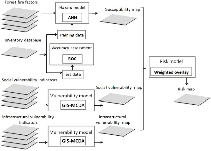
The methodologies (see Figure1) and the experimental results are organized in the following sections. Further descriptions and discussions regarding the resulting maps can be found in the discussions and conclusion section.

Fire 2019, 2, x FOR PEER REVIEW 4 of 26

 Validating the performances of the ANN method using the receiver operating characteristics (ROC) curve and the root mean square error (RMSE).

The methodologies (see Figure 1) and the experimental results are organized in the following sections. Further descriptions and discussions regarding the resulting maps can be found in the discussions and conclusion section.

Figure 1. Methodology scheme and workflow.

2.1. Study Area

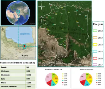
The case study was the forestry area of Amol County in the Mazandaran province of northern Iran (Figure 2). Our study area has an expanse of 646 km2 _{and is essential for its natural forests and}

as one of the common recreational centres of the country. The study area attracts tourists from all over the country. The altitude ranges from 100 m in valleys to approximately 2500 m above mean sea level in mountainous areas in the southern part. Other topographical and environmental characteristics are described in Table 1. The study area is potentially vulnerable to forest fires, which are considered as a common problem in the region. There are more than 20 villages in the study area, mostly in valleys and some located in remote forest areas. The most common activity among the population is animal husbandry. However, there are also orchards, including walnuts and apple gardens, and even some agricultural activities.

Figure 1.Methodology scheme and workflow.

2.1. Study Area

Fire2019,2, 50 5 of 27

Fire 2019, 2, x FOR PEER REVIEW 5 of 26

Figure 2. Study area with polygons indicating the approximate location of regions burned between 2012 and 2017.

2.2. Data Used in the Analysis

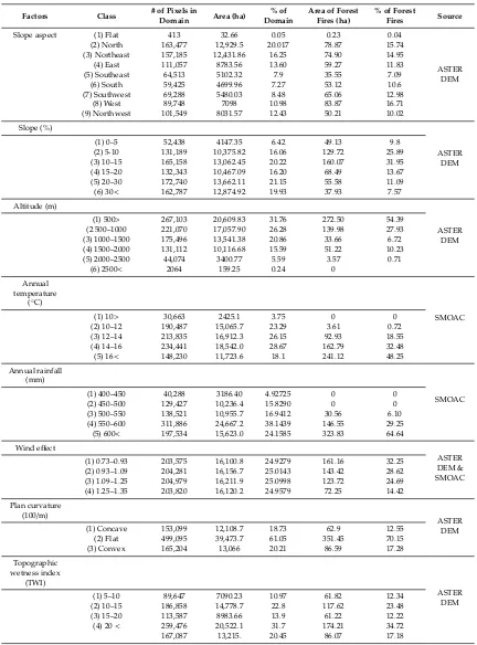
To generate the forest fire susceptibility map of our study area, 16 relevant factors including environmental variables were considered as forest fire occurrence data.

The relevant topographic factors are slope aspect, slope, altitude, plan curvature, landform, and the topographic wetness index (TWI). The meteorological factors are annual temperature, potential solar radiation, and wind effect. The considered vegetation factor was the normalized difference vegetation index (NDVI). The NDVI factor was created for the high vegetated summer period, applying Landsat-8 Operational Land Imagery (OLI) 30 m resolution, retrieved from the USGS archive (http://earthexplorer.usgs.gov). The human-made factors are the distance to the nearest village, land use, and the distance to roads and recreational areas. The hydrological factors are annual rainfall and the distance to streams (see Table 1).

The topographic factors were derived from the Advanced Spaceborne Thermal Emission and Reflection Radiometer (ASTER) (NASA, California Institute of Technology, USA) Global Digital Elevation Model (GDEM) with an approximate resolution of 30 m. Related topographic factors are considered as important forest fire factors that impact the fire’s separate pattern in forests [47]. These factors have been widely used for forest fire susceptibility mapping [48]. The slope factor is essential because increasing in slope angle results in fire spreading more quickly [27]. Since usually north-facing slopes are colder and moister than those of south, the risk of forest fire on south-north-facing slopes is higher [49]. The presence of higher moister at higher altitude shows the importance of this factor [50]. The factor of wind effect was generated by three different factors, including the degree of wind direction, wind speed (m/s), and altitude layer [51]. The solar radiation varies from nearly 0.3

KWH m,⁄ to more than 1.8 KWH m⁄ and this range is classified in five classes based on natural Figure 2.Study area with polygons indicating the approximate location of regions burned between 2012 and 2017.

2.2. Data Used in the Analysis

To generate the forest fire susceptibility map of our study area, 16 relevant factors including environmental variables were considered as forest fire occurrence data.

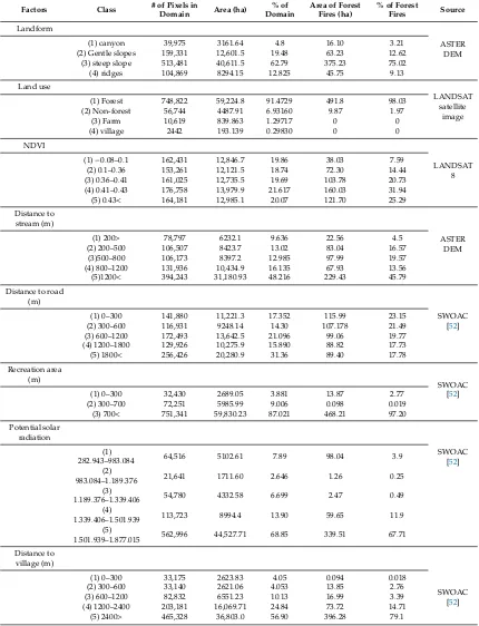
The relevant topographic factors are slope aspect, slope, altitude, plan curvature, landform, and the topographic wetness index (TWI). The meteorological factors are annual temperature, potential solar radiation, and wind effect. The considered vegetation factor was the normalized difference vegetation index (NDVI). The NDVI factor was created for the high vegetated summer period, applying Landsat-8 Operational Land Imagery (OLI) 30 m resolution, retrieved from the USGS archive (http:

//earthexplorer.usgs.gov). The human-made factors are the distance to the nearest village, land use,

and the distance to roads and recreational areas. The hydrological factors are annual rainfall and the distance to streams (see Table1).

Fire2019,2, 50 6 of 27

Table 1.Forest fire relevant factors, classes by corresponding areas, and percent of the burned areas in each class.

Factors Class # of Pixels in

Domain Area (ha)

% of Domain

Area of Forest Fires (ha)

% of Forest

Fires Source

Slope aspect (1) Flat 413 32.66 0.05 0.23 0.04

ASTER DEM

(2) North 163,477 12,929.5 20.017 78.87 15.74

(3) Northeast 157,185 12,431.86 16.25 74.90 14.95

(4) East 111,057 8783.56 13.60 59.27 11.83

(5) Southeast 64,513 5102.32 7.9 35.55 7.09

(6) South 59,425 4699.96 7.27 53.12 10.6

(7) Southwest 69,288 5480.03 8.48 65.06 12.98

(8) West 89,748 7098 10.98 83.87 16.71

(9) Northwest 101,549 8031.57 12.43 50.21 10.02

Slope (%)

ASTER DEM

(1) 0–5 52,438 4147.35 6.42 49.13 9.8

(2) 5-10 131,189 10,375.82 16.06 129.72 25.89

(3) 10–15 165,158 13,062.45 20.22 160.07 31.95

(4) 15–20 132,343 10,467.09 16.20 68.49 13.67

(5) 20–30 172,740 13,662.11 21.15 55.58 11.09

(6) 30< 162,787 12,874.92 19.93 37.93 7.57

Altitude (m)

ASTER DEM (1) 500> 267,103 20,609.83 31.76 272.50 54.39

(2 500–1000 221,070 17,057.90 26.28 139.98 27.93

(3) 1000–1500 175,496 13,541.38 20.86 33.66 6.72

(4) 1500–2000 131,112 10,116.68 15.59 51.22 10.23

(5) 2000–2500 44,074 3400.77 5.59 3.57 0.71

(6) 2500< 2064 159.25 0.24 0

Annual temperature

(◦

C)

SMOAC

(1) 10> 30,663 2425.1 3.75 0 0

(2) 10–12 190,487 15,065.7 23.29 3.61 0.72

(3) 12–14 213,835 16,912.3 26.15 92.93 18.55

(4) 14–16 234,441 18,542.0 28.67 162.79 32.48

(5) 16< 148,230 11,723.6 18.1 241.12 48.25

Annual rainfall (mm)

SMOAC

(1) 400–450 40,288 3186.40 4.92725 0 0

(2) 450–500 129,427 10,236.4 15.8290 0 0

(3) 500–550 138,521 10,955.7 16.9412 30.56 6.10

(4) 550–600 311,886 24,667.2 38.1439 146.55 29.25 (5) 600< 197,534 15,623.0 24.1585 323.83 64.64 Wind effect

ASTER DEM & SMOAC (1) 0.73–0.93 203,575 16,100.8 24.9279 161.16 32.25

(2) 0.93–1.09 204,281 16,156.7 25.0143 143.42 28.62 (3) 1.09–1.25 204,979 16,211.9 25.0998 123.72 24.69 (4) 1.25–1.35 203,820 16,120.2 24.9579 72.25 14.42 Plan curvature

(100/m)

ASTER DEM

(1) Concave 153,099 12,108.7 18.73 62.9 12.55

(2) Flat 499,095 39,473.7 61.05 351.45 70.15

(3) Convex 165,204 13,066 20.21 86.59 17.28

Topographic wetness index

(TWI)

ASTER DEM

(1) 5–10 89,647 7090.23 10.97 61.82 12.34

(2) 10–15 186,858 14,778.7 22.8 117.62 23.48

(3) 15–20 113,587 8983.66 13.9 61.22 12.22

(4) 20< 259,476 20,522.1 31.7 174.21 34.72

Fire2019,2, 50 7 of 27

Table 1.Cont.

Factors Class # of Pixels in

Domain Area (ha)

% of Domain

Area of Forest Fires (ha)

% of Forest

Fires Source

Landform

ASTER DEM

(1) canyon 39,975 3161.64 4.8 16.10 3.21

(2) Gentle slopes 159,331 12,601.5 19.48 63.23 12.62 (3) steep slope 513,481 40,611.5 62.79 375.23 75.02

(4) ridges 104,869 8294.15 12.825 45.75 9.13

Land use

LANDSAT satellite

image

(1) Forest 748,822 59,224.8 91.4729 491.8 98.03

(2) Non-forest 56,744 4487.91 6.93160 9.87 1.97

(3) Farm 10,619 839.863 1.29717 0 0

(4) village 2442 193.139 0.29830 0 0

NDVI

LANDSAT 8

(1)−_{0.08–0.1 162,431 12,846.7 19.86 38.03 7.59}

(2) 0.1–0.36 153,261 12,121.5 18.74 72.30 14.44

(3) 0.36–0.41 161,025 12,735.5 19.69 103.78 20.73 (4) 0.41–0.43 176,758 13,979.9 21.617 160.03 31.94 (5) 0.43< 164,181 12,985.1 20.07 121.70 25.29 Distance to

stream (m)

ASTER DEM

(1) 200> 78,797 6232.1 9.636 22.56 4.5

(2) 200–500 106,507 8423.7 13.02 83.04 16.57

(3)500–800 106,173 8397.2 12.985 97.99 19.57

(4) 800–1200 131,936 10,434.9 16.135 67.93 13.56

(5)1200< 394,243 31,180.93 48.216 229.43 45.79 Distance to road

(m)

SWOAC [52]

(1) 0–300 141,880 11,221.3 17.352 115.99 23.15

(2) 300–600 116,931 9248.14 14.30 107.178 21.49

(3) 600–1200 172,493 13,642.5 21.096 99.06 19.77

(4) 1200–1800 129,926 10,275.9 15.890 88.82 17.73 (5) 1800< 256,426 20,280.9 31.36 89.40 17.78 Recreation area

(m) _SWOAC

[52]

(1) 0–300 32,430 2689.05 3.881 13.87 2.77

(2) 300–700 72,251 5985.99 9.006 0.098 0.019

(3) 700< 751,341 59,830.23 87.021 468.21 97.20 Potential solar

radiation

SWOAC [52] (1)

282.943–983.084 64,516 5102.61 7.89 98.04 3.9

(2)

983.084–1.189.376 21,641 1711.60 2.646 1.26 0.25

(3)

1.189.376–1.339.406 54,780 4332.58 6.699 2.47 0.49 (4)

1.339.406–1.501.939 113,723 8994.4 13.90 59.65 11.9 (5)

1.501.939–1.877.015 562,996 44,527.71 68.85 339.51 67.71 Distance to

village (m)

(1) 0–300 33,175 2623.83 4.05 0.094 0.018

SWOAC [52]

(2) 300–600 33,140 2621.06 4.053 13.85 2.76

(3) 600–1200 82,832 6551.23 10.13 16.99 3.39

(4) 1200–2400 203,181 16,069.71 24.84 73.72 14.71 (5) 2400> 465,328 36,803.0 56.90 396.28 79.1

Fire2019,2, 50 8 of 27

Fire 2019, 2, x FOR PEER REVIEW 8 of 26

Fire2019,2, 50 9 of 27

Fire 2019, 2, x FOR PEER REVIEW 9 of 26

Fire2019,2, 50 10 of 27

Fire 2019, 2, x FOR PEER REVIEW 10 of 26

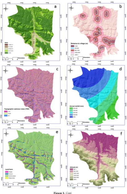
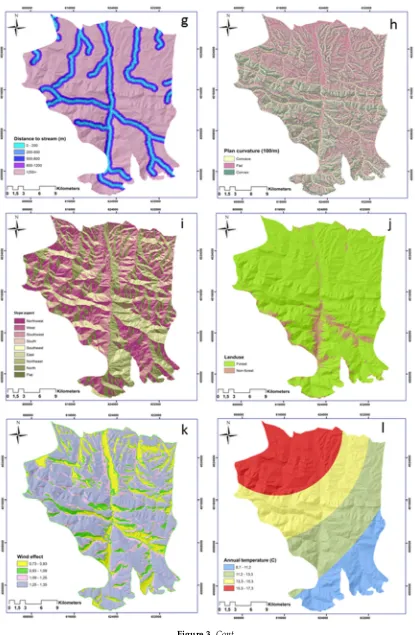
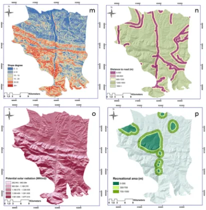
Figure 3. Sixteen input forest fire factors used in the artificial neural network (ANN) method: (a) normalized difference vegetation index (NDVI), (b) distance to village, (c) topographic wetness index (TWI), (d) annual rainfall, (e) land form, (f) altitude, (g) distance to stream, (h) plan curvature, (i) slope aspect, (j) land use, (k) wind effect, (l) annual temperature, (m) slope degree, (n) distance to road, (o) potential solar radiation, (p) recreational areas.

2.3. Data Generation for Training and Testing

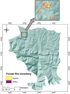
In this subsection, we summarise the generation process of our training and test data. The polygons of the forest fires in the study area were generated based on GPS data (obtained from the state wildlife organization) along with the hotspots of Moderate Resolution Imaging Spectroradiometer (MODIS) (NASA, Goddard Space Flight Center, Maryland, USA). Using MODIS fire detection data is common, and used in several current studies, to specify the location and the time of forest fires [55–57]. Our investigation resulted in 34 forest fire GPS polygons that were evaluated by the MODIS sensor during the 2012–2017 timeframe (see Figure 1). Of these forest fire polygons, we randomly selected 70% (12,195 pixels) as training data and 30% (5226 pixels) for the validation section using ten-fold cross-validation (CV) (see Figure 4). We used the ten-fold CV approach to deal with the randomness adverse effects on the forest fire susceptibility modelling [58]. The forest fire polygons were randomly divided into ten folds of approximately 1742 pixels. Technically speaking, if we have the dataset D and divide it randomly into k number of the same folds of 𝐷 , 𝐷 , …, 𝐷 . Then, the model is trained k times and each time t ∈ (1, 2, …, k). For the time of t, the model is run with the dataset of D lacking of the subset of 𝐷, and validated with 𝐷 [59]. Thus,

Figure 3. Sixteen input forest fire factors used in the artificial neural network (ANN) method: (a) normalized difference vegetation index (NDVI), (b) distance to village, (c) topographic wetness index (TWI), (d) annual rainfall, (e) land form, (f) altitude, (g) distance to stream, (h) plan curvature, (i) slope aspect, (j) land use, (k) wind effect, (l) annual temperature, (m) slope degree, (n) distance to road, (o) potential solar radiation, (p) recreational areas.

2.3. Data Generation for Training and Testing

Fire2019,2, 50 11 of 27

and each timet∈_{(1, 2,}. . ._{, k). For the time oft, the model is run with the dataset ofDlacking of the}

subset ofDt, and validated withDt[59]. Thus, three of the folds were chosen each time for validation and other seven folds were used for training the model. This process was repeated for every fold in our inventory dataset of the forest fire. Although most researchers used ten folds, the number of folds in the spatial applications is often selected by the user without any empirical evidence. The authors of Reference [60] used a three-fold CV approach. Whereas, in Reference [61] they selected a five-fold for their training and validation aims. We selected ten folds for the cross validation because of the large volume of our inventory dataset. Therefore, the outputs of the forest fire susceptibility modelling in this study were based on the ten-fold CV that resulted in the highest accuracies in both the training and the validation sections (see Sections3.1and4.1).

Fire 2019, 2, x FOR PEER REVIEW 11 of 26

three of the folds were chosen each time for validation and other seven folds were used for training the model. This process was repeated for every fold in our inventory dataset of the forest fire. Although most researchers used ten folds, the number of folds in the spatial applications is often selected by the user without any empirical evidence. The authors of Reference [60] used a three-fold CV approach. Whereas, in Reference [61] they selected a five-fold for their training and validation aims. We selected ten folds for the cross validation because of the large volume of our inventory dataset. Therefore, the outputs of the forest fire susceptibility modelling in this study were based on the ten-fold CV that resulted in the highest accuracies in both the training and the validation sections (see Sections 3.1 and 4.1).

Figure 4. Forest fire inventory divided randomly to training and testing.

3.1. Forest Fire Susceptibility Mapping Using Artificial Neural Network (ANN)

The ANN method is considered to be one of the most commonly used ML methods to assess susceptible areas of forest fires [28]. Generally, ANNs mimic human brain performance, and they can solve complex nonlinear problems with multiple numbers of components and variables [62]. ANNs also can find patterns and discover the trends of complex issues [63]. In the present study, to create an index for assessing forest fires, a model was used with the ANN method using a multilayer perceptron (MLP) architecture and trained with the backpropagation algorithm (BPA), which is considered as the most common algorithm for the ANN method. The MLP architecture consists of several hidden layers between the input and output layers. The number of hidden layers of a neural network depends on the complexity of the problem [64]. For our case, the feed-forward network was

Figure 4.Forest fire inventory divided randomly to training and testing.

3. Workflow

3.1. Forest Fire Susceptibility Mapping Using Artificial Neural Network (ANN)

Fire2019,2, 50 12 of 27

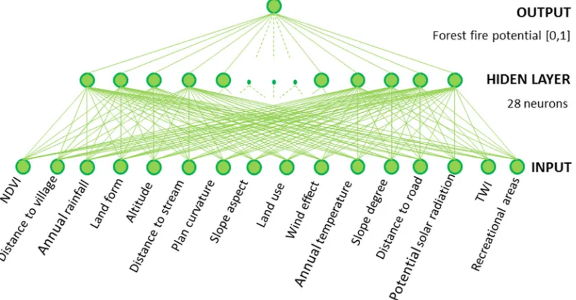
architecture and trained with the backpropagation algorithm (BPA), which is considered as the most common algorithm for the ANN method. The MLP architecture consists of several hidden layers between the input and output layers. The number of hidden layers of a neural network depends on the complexity of the problem [64]. For our case, the feed-forward network was made up of an input layer with 16 neurons (input factors), one hidden layer (28 neurons) and one output layer as a network structure of 16-28-1 (see Figure5). The number of 28 hidden layers was determined through 3-fold CV on a range of (12, 18, 28 neurons).

Fire 2019, 2, x FOR PEER REVIEW 12 of 26

made up of an input layer with 16 neurons (input factors), one hidden layer (28 neurons) and one output layer as a network structure of 16-28-1 (see Figure 5). The number of 28 hidden layers was determined through 3-fold CV on a range of (12, 18, 28 neurons).

Figure 5. The architecture of the neural network model for Forest fire.

The training dataset consists of forest fire and non-forest fire areas containing sixteen inputs, namely, slope aspect, slope degree, altitude, plan curvature, landform, TWI, annual temperature, potential solar radiation, wind effect, NDVI, distance to village, land use, distance to road, recreational areas, annual rainfall, and distance to stream. Mapping forest fire susceptibility using the described ANN method consists of a three-stage process, namely, training, allocation, and testing the values of each pixel of an input layer were presented to the neural network along with the values of the training dataset. Each of the fifteen neurons in the input layer (𝑦 , 𝑦 , …, 𝑦 ) characterized an attribute of the input data and transferred the signal to the corresponding connected neurons (𝑧 , 𝑧 ,…, 𝑧 ) in our hidden layer. The total input signal to the 𝑧 neuron (in the hidden layer) can be defined as Equation (1) [65].

𝑧(𝑖𝑛) = 𝑢 𝑦 + 𝑢 (1)

where, 𝑢 is the weighted value that came from the 𝑖 input neuron and 𝑢 is the corresponding bias value. The activation of each neuron in this layer is computed separately and transferred to the next neuron, which is the output neuron. Equation (2) presents how the output neuron O catches the values from the hidden layer.

𝑂(𝑖𝑛) = 𝑧 𝑤 + 𝑤 (2)

where, zj is the jth resulting value from Equation (1), wj is the weight and wo is the corresponding bias

value [66]. The calculated output value from the ANN method is compared with the forest fire pixel values, which are considered as the target value t. The comparison is done for every terrain unit until the overall error between t and the derived output value o is acceptable (minimum). The forest fire pixel values, which are considered as the target value t, were not used for training data earlier in the process. The momentum parameter avoids divergence during the process, and has a useful role in increasing the speed of convergence [67]. All weightings were updated by the backward process during each cycle in order to minimize the error. The common activation functions used for the ANN

Figure 5.The architecture of the neural network model for Forest fire.

The training dataset consists of forest fire and non-forest fire areas containing sixteen inputs, namely, slope aspect, slope degree, altitude, plan curvature, landform, TWI, annual temperature, potential solar radiation, wind effect, NDVI, distance to village, land use, distance to road, recreational areas, annual rainfall, and distance to stream. Mapping forest fire susceptibility using the described ANN method consists of a three-stage process, namely, training, allocation, and testing the values of each pixel of an input layer were presented to the neural network along with the values of the training dataset. Each of the fifteen neurons in the input layer (y1,y2,. . .,y16) characterized an attribute of the input data and transferred the signal to the corresponding connected neurons (z1,z2,. . .,z9) in our hidden layer. The total input signal to thezxneuron (in the hidden layer) can be defined as Equation (1) [65].

z(in)_x= 16 X

1

uixyi+ ux (1)

where,uixis the weighted value that came from theithinput neuron anduxis the corresponding bias value. The activation of each neuron in this layer is computed separately and transferred to the next neuron, which is the output neuron. Equation (2) presents how the output neuronOcatches the values from the hidden layer.

O(in) = 28 X

1

zjwj+ wo (2)

Fire2019,2, 50 13 of 27

values, which are considered as the target valuet,were not used for training data earlier in the process. The momentum parameter avoids divergence during the process, and has a useful role in increasing the speed of convergence [67]. All weightings were updated by the backward process during each cycle in order to minimize the error. The common activation functions used for the ANN method are hyperbolic tangent and the logistic functions. For our case, the logistic function (see Equation (3)) was selected, as the output of the function is an interval value varying from 0 to 1, which is more preferable for a susceptibility map.

f(xi) = (1+ e

−_xi

)−1 (3)

The transfer function f was a nonlinear sigmoid function that was used to the weighted sum of the input data before the next layer. Different learning rates were applied from 0.1 to 0.9 and the learning rate of 0.9 got a higher accuracy in forest fire susceptibility mapping. Several iterations were tested, and 1000 iterations were selected as the optimal one in terms of both of accuracy and cost. Finally, the hazard map was generated from the output values of the ANN method. The pixels with values close to 1 have a higher probability of forest fires occurring and pixels with low values indicate safer areas.

3.2. Social/Infrastructural Vulnerability Indexes

Choice of Indicators

There are several social indicators, such as education level, age, gender, and access to government facilities and health services, that can indicate the level of a community’s ability to be deal with and recover from natural hazards like forest fires [18,38]. In this research, 22 social vulnerability indicators were selected based on the living standards and local conditions in our study area (see Table 3). The dataset was obtained from the Iranian Bureau of Statistics 2017 census. Our study area consists of 20 villages with an estimated population of 2887. The least populated village only has 11 inhabitants, and the most populated one has a population exceeding 1650. Since all villages belong to the same county, they have approximately equal access to government support and facilities. However, there are some indicators that vary between villages, e.g., the percent of the vulnerable population under 14 years of age or 65 and older, and the percent of the unemployed people.

In this study, we also consider several susceptible areas and valued infrastructural assets and resources within the study area that are prone to forest fires (see Table 4). There are also some people who live temporarily (seasonal) or permanently in these areas. Roads and forest parks, for instance, are frequented by visitors from all over the country and, mainly, from Tehran during the summer time. On the other hand, since the occupation of most people in our study area is the livestock sector, there are several barns in the depths of the forest areas, most of which are illegal. These barns are used to keep the livestock during the fall and winter. As they are usually established in remote areas, it is more likely that they are surrounded by or even engulfed in a fire during a forest fire event. Thus, eleven infrastructural vulnerability indicators were also selected based on the situation of our study area. To consider the spatial information of both the social and infrastructure indicators, the datasets need to be transferred to a GIS environment and aggregated to layers. However, the indicators are represented by different measurement scales (i.e., percentage and number) [68]. Thus, before being aggregated, they were transformed into a continuous scale of common units with a linear standardisation method.

3.3. Aggregation of Different Indicators Using Geographic Information System Multi-Criteria Decision Making (GIS-MCDM)

Fire2019,2, 50 14 of 27

we consider the general context of vulnerability, their significance depends on the type of natural hazard. MCDAs are practical approaches for a wide range of complex decision-making systems.

The set of X = (x1,x2,. . .,xn) was considered with n number of selected social indicators. Experts compared each pair of indicators (xi andxj) inX. A value (aij) can also result from the ratio of their weightings [70]. If the social indicatorxiis preferred toxj,thenaij>1and, conversely, ifxjis preferred toxithenaij<1. A verbal description of the importance, introduced by Saaty to compare various indicators in a pairwise manner, is given in Table2. The values vary from 1, for equal importance, to 9, for extreme importance. Foriandj=1,2,. . . ,n, and anyaij >0we haveaji= _a1_{i j} (reciprocal property). The resulting indicator weightings (w1, w2, w3,. . .,wn) have two conditions, namely: 0≤_wk≤_{1 and}

n

P

k=1 wk =1

Therefore, the pairwise comparisons are structured in a matrix, and the matrix’s elements are between 1/9 and 9. The AHP method can integrate both quantitative and qualitative dimensions of a decision-making problem [71]. The method is also able to differentiate between our indicators and to support the comparison of the performance of them with few calculations [72].

                                   

1 a12 . . . 1

a12 1 . . .

. . . 1

a1i . . . a1j . . . a1n a2i . . . a2j . . . a2n

. . . .

1

a1i

1

a2i . . .

. . . .

1

a1j

. . .

1

a1n

1

a2j

. . .

1

a2n

. . . . . . . . .

1 . . . ai j . . . ain

. . . 1 . . . . 1

ai j

. . . 1 ain . . . . . . . . . 1 . . . 1 ajn . . . 1 . . . ajn . . . 1                                     (4)

Table 2.The scale of Intensity of Importance (IOI) [73].

IOI Description

1 Equal importance

3 Moderate importance

5 Strong or essential importance

7 Very strong or demonstrated

importance

9 Extreme importance

2,4,6,8 Intermediate values

Reciprocals Values for inverse comparison

Fire2019,2, 50 15 of 27

Table 3. Social vulnerability indicators and resulting analytic hierarchy process (AHP) weights for each indicator.

Indicators Sub-Indicators AHP Weights

Education

Speaking the official language (Persian) as a second language with limited

Persian proficiency (%) 0.045

Population that does not have any level of formal education or instruction

(%) 0.051

Population that does not have access to school\_{high school (%) 0.040}

Housing

Houses older than ten years (%) 0.041

Houses without steel or concrete skeleton (%) 0.059

Houses with an area less than 75 (%) 0.007

Houses without garbage collection service (%) 0.006

Age

Population under 14 years or 65 and older (%) 0.064

Female

Female population (%) 0.035

Female-headed households (%) 0.047

Health services

The population that does not have access to health centres (%) 0.072 The population that does not have access to a family doctor (%) 0.021 The population that does not have access to a lab and pharmacy (%) 0.025

Facilities

Households without access to the public electricity network (%) 0.073 Households without access to drinking water from the public system (%) 0.050 Households without access to the public gas pipeline network (%) 0.033 Households without access to the sewerage system (%) 0.007 Households without access to the internet network (%) 0.034 The population that does not have access to the public transportation

system (%) 0.012

Fire station 0.201

Police station 0.034

Occupation

Unemployed population (%) 0.040

Table 4. Infrastructural vulnerability indicators and resulting AHP weights for each indicator. All distances measures are based on meters.

Indicators Sub-Indicators AHP Weights

Industrial area

Mines 0.033

Livestock and poultry farming (nests) 0.242

The national power line 0.035

Recreational area

Forest parks with some amenities such as shelters for

temporary stays in the woods 0.103

Restaurants and buffets 0.067

Motels and Inns 0.095

Roads

The main road from Tehran to northern Iran mainly

used for transporting essential goods and tourists 0.060 Gravel roads mainly used by the local population

and illegal hunters 0.041

Agricultural area

Orchards, including walnut and apple gardens 0.136

Irrigated agriculture 0.088

Fire2019,2, 50 16 of 27

4. Results

4.1. The Predictive Performances and Resulting Hazard Map

In this subsection, we sought to spatially represent regions on the study area associated with high susceptibility of forest fire. The ML component of the ANN method was used for susceptibility modelling and mapping. For this goal, the output values of the ANN method were derived through GIS spatial analysis and data aggregation models. As we trained the ANN method with burned area polygons which including also ignition locations, the resulting susceptibility maps represent a measure of the likelihood of ignition and the probability of spreading of forest fires based on considered conditioning factors. Figure6shows the results of the forest fire susceptibility map from the applied ML method. Concerning the spatial distribution, the probability of forest fires is higher in northern and central areas where local people and tourists have accessibility to low-elevation forests. The natural breaks classification method (or Jenks optimization) used in this study generates classes of similar values separated by breakpoints. This is a common and effective method for categorizing the susceptibility mapping results when we interpret values close to each class boundary (e.g., values between “Low” and “Moderate” probability) [77]. Table5depicts the area and the percentage of each class of the resulting forest fire map. The RMSE [78,79] was used to assess the model performance and Equation (5) depicts the calculation:

RMSE = (1 N

n

X

i=1

(ei−ei)2)

0.5

(5)

Fire2019,2, 50 17 of 27

Fire 2019, 2, x FOR PEER REVIEW 16 of 26

categorizing the susceptibility mapping results when we interpret values close to each class boundary (e.g., values between ‘‘Low’’ and ‘‘Moderate’’ probability) [77]. Table 5 depicts the area and the percentage of each class of the resulting forest fire map. The RMSE [78,79] was used to assess the model performance and Equation (5) depicts the calculation:

RMSE = (1

𝑁 (𝑒 − 𝑒 ) ) . (5)

where, 𝑒 and 𝑒 are the 𝑖 observed and results of the ANN method, respectively. The best derived RMSE

value based on the ten-fold CV was 0.145. Generally, small values of the RMSE show better performance of the prediction model [80]. However, in order to validate the resulting forest fire susceptibility map, we conducted a validation process based on the 5226 forest fire pixels (see Section 2.3) that were not used for training in the utilized ANN method. The validation step aims to ensure the accuracy of the resulting hazard map [76]. The spatial success of the hazard map was examined through the receiver operating characteristics (ROC) curve, which is a common method for characterizing the quality of deterministic and probabilistic prediction methods. This curve shows the trade-off between the false positive rate and the true positive rate, by plotting the false positive rate on the X axis and the true positive rate on the Y axis [24]. If the area under the curve (AUC) is close to one, this indicates that the prediction model has a high quality. Our ROC curve consists of 5226 pixels reflecting known and observed (by MODIS) forest fires in the study area. Figure 7 shows the results of comparing the observed forest fires with the forest fire susceptibility map. The results of the ROC method for our hazard map indicated accuracies fluctuate around 74% and the highest one based on the ten-fold CV was an accuracy of more than 80%. This result was used to further analysis of the risk map generating.

Figure 6.Forest fire susceptibility map.

Table 5.The AHP weights for the resulting maps and corresponding classes with the absolute area and the relative percentage of the region compared to the whole study area.

Resulted Maps AHP Weights Classes Area (ha) Area (%) AHP Weights

Forest fire 0.53 Very low 26,665.96 41.31 0.05 susceptibility Low 23,257.7 36.03 0.08 Moderate 14,399.16 22.31 0.22 High 215.28 0.33 0.64

CR=0.03 Social vulnerability 0.29 Very low 62,998.69 97.41 0.6

Low 508.63 0.78 0.15 Moderate 177.87 1.52 0.26 High 983.73 2.27 0.42

CR=0.03 Infrastructural 0.16 Very low 29,377.66 45.43 0.078

vulnerability Low 28,688.23 41.36 0.15 Moderate 6445.09 9.96 0.26 High 149.32 3.23 0.5

Fire2019,2, 50 18 of 27

Fire 2019, 2, x FOR PEER REVIEW 17 of 26

Figure 6. Forest fire susceptibility map.

Figure 7. The receiver operating characteristics (ROC) curve and sensitivity value for the resulting hazard map.

4.2. Social/Infrastructural Vulnerability Mapping

To obtain social and infrastructural vulnerability maps, the weightings derived from the AHP method were used for data aggregation within a GIS environment. A buffer zone of 200 m was used for residential areas, and different multibuffers were used for infrastructural indicators based on their importance regarding forest fires. All indicators were prepared as GIS layers and then aggregated with a weighted overlay technique. Figure 8a and b present the vulnerability maps resulting from social and infrastructural indicators, respectively. The social vulnerability map was classified into five classes of vulnerability using the natural breaks classification method. The infrastructural vulnerability map, on the other hand, was classified into four categories of vulnerability using the same method of classification. The natural breaks classification method and the number of classes for categorisation were selected based on literature and expert knowledge. Table 5 shows the area of the respective classes for both the social and infrastructural vulnerability maps.

Figure 7.The receiver operating characteristics (ROC) curve and sensitivity value for the resulting hazard map.

4.2. Social/Infrastructural Vulnerability Mapping

Fire2019,2, 50 19 of 27

Fire 2019, 2, x FOR PEER REVIEW 18 of 26

(a)

(b)

Figure 8. Resulting (a) infrastructural and (b) social vulnerability map.

4.3. Generation of the Risk Map

Forest fires will have adverse impacts on different types of elements-at-risk. Thus, it is crucial to consider the forest fire threat for different sectors [9]. Moreover, all related stakeholders should be involved in a comprehensive forest fire risk mapping [81]. For this reason, we considered 16 relevant

Fire2019,2, 50 20 of 27

4.3. Generation of the Risk Map

Forest fires will have adverse impacts on different types of elements-at-risk. Thus, it is crucial to consider the forest fire threat for different sectors [9]. Moreover, all related stakeholders should be involved in a comprehensive forest fire risk mapping [81]. For this reason, we considered 16 relevant forest fire factors, 22 social vulnerability indicators, and 11 infrastructural indicators, to ensure the inclusion of the most important factors that play a role in the forest fire risk assessment in our study area. The hazard map was generated using an ANN method because we had access to sufficient inventory data for training and testing matters. However, social and infrastructural vulnerability maps were created using a GIS-MCDA method, which is one of the more common methods for vulnerability and susceptibility mapping in a wide range of disciplines [82]. Mapping areas with a high probability of forest fire risk can be carried out by aggregating the hazard map and the social/infrastructural vulnerability maps. The GIS-MCDA approach was, again, used to specify the relative significance of indicators and to aggregate the forest fire susceptibility, infrastructural vulnerability, and social vulnerability to generate the final risk map. By using the AHP method, we calculated the weights resulting from the pairwise comparison matrices for the three resulting maps and the corresponding classes. The pairwise comparison matrices were filled by the same experts who were mentioned in Section3.3. All resulting maps were prepared as GIS layers and then overlaid with the respective AHP weights, which were almost 54% for the forest fire susceptibility, 30% for the social vulnerability, and 16% for the infrastructural vulnerability layer (see Table5). The final forest fire risk map was classified by natural breaks (‘Jenks’) and is represented in Figure9via four classes. This classification method yields classes that are based on natural groupings of the pixel values. Class breaks are specified in a way that the resulting groups are most similar and the differences between classes are maximized. Area and percentage of the forest fire risk map classes are represented in Table6. The forest fire risk map reflects both the forest fire susceptibility (including the likelihood of ignition and the probability of spreading) and social/infrastructural vulnerability. The forest fire risk map shows that the slope aspect factor played a key role in the susceptibility of spreading, consequently raises the forest fire risk. For the other aspects, the susceptibility of a forest fire occurring is high due to the impact of other conditioning factors. Therefore, the applied ANN method could be trained well with all factors based on the inventory forest fire data and succeeded in predicting high forest fire susceptible areas. High temperature and low rainfall in the northern regions of the study area obviously increased the susceptibility of the forest fire ignition and spread. Although steep areas are generally more susceptible for forest fires, the human activity close to the main road (even with more moderate slopes in the northern parts) had a primary effect on the susceptibility and the risk map. The interaction of settlement areas (high social vulnerability) and infrastructural vulnerable areas with the high and moderate forest fire susceptibility resulted in high risk regions in the forest fire risk map (see Figure9).

Table 6.Area and percentage of forest fire risk classes compared to the whole study area.

Resulted Map Classes Area (ha) Area (%)

Forest fire susceptibility Very low 24,930.87 38.62

Low 23,919.53 37.06

Moderate 14,958.09 23.17

Fire2019,2, 50 21 of 27

Fire 2019, 2, x FOR PEER REVIEW 20 of 26

Figure 9. Forest fire risk map.

Table 6. Area and percentage of forest fire risk classes compared to the whole study area.

Resulted Map Classes Area (ha) Area (%)

Forest fire susceptibility Very low 24,930.87 38.62

Low 23,919.53 37.06 Moderate 14,958.09 23.17 High 729.61 1.14

5. Discussion and Conclusion

Mapping the forest fire risk posed to human life and properties is an essential component of emergency land management, forest fire prevention, mitigation of adverse impacts, and response and recovery management [83]. As already discussed in the introduction section, forest fire susceptibility maps have often been used to priorities investments in forest fire prevention, and also for preparation planning. However, even considering social vulnerabilities leads to more effective forest fire risk management [84]. Since such risk maps can illustrate the location of the elements-at-risk, besides communities who have a lower capacity to deal with the fire and the spatial correlations between communities and fires, they are also more useful for land managers and firefighters for emergency planning in combating fires in real time. Therefore, a comprehensive forest fire mitigation and disaster management plan should concentrate on areas where there is an overlap between populations and their more vulnerable properties and a higher forest fire risk. In this regard, the forest fire susceptibility map of our study was generated using environmental variables. We considered the most available factors and prepared them as input data for the model. Training and testing data were generated using field survey GPS polygons and MODIS hotspot data. The field survey was done by the SWOAC [52]. According to the literature, a wide range of approaches have been used to predict areas with potential susceptibility to forest fires. Thus, different methods have been applied by various researchers to explore the potential role of relative factors that point to fire events. In this research, we generated a model using an ANN method with an MLP architecture that

Figure 9.Forest fire risk map.

5. Discussion and Conclusion

Fire2019,2, 50 22 of 27

in terms of the number of the forest fires. The GPS dataset is more reliable regarding the shape of the polygons of burned areas because of the low resolution of MODIS. Consequently, the integration of both sources resulted in a more reliable inventory dataset of the location and the extension area of the wildfires. Nevertheless, the resolution of the resulting inventory dataset was not the same as that of the input data. Therefore, this difference in the resolution resulted in some uncertainties, which are difficult to quantify.

The model was developed and trained based on the previous forest fire events between 2012 and 2017, and the relevant factors contributing to the forest fire. The performance of the model was evaluated by the RMSE, and the resulting forest fire susceptibility map was validated using the ROC curve. Both of these measures showed acceptable accuracies of the results of the model. The resulting forest fire susceptibility map with the highest accuracy revealed that the southern part of our study area is more susceptible to forest fires in the future. This matter illustrates that the factors of annual rainfall and annual mean temperature play an important role by creating extreme dryness, which is a crucial factor determining forest fires [85]. The areas with high forest fire susceptibility also have a close spatial correlation with the previously recorded forest fire events.

Although environmental variables contributing to the forest fire played an essential role in the assessment of susceptible forest fire areas, they are not the only reason for both forest fire susceptibility and risk. As some of the forest fires in in our case study are reported to be a result of human activity and the local people in particular SWOAC [52], considering the areas and some specific sites of human activity such as recreational areas can help to have a better understanding of the results of the forest fire susceptibility and risk. The distance from population concentration is considered to be relevant to human activity. Therefore, the closer regions to the settlements and population concentration can indicate a higher presence of human activity and consequently more susceptibility and risk of forest fire [31]. Thus, the population density and social vulnerability indicators were used, which were gained from different sources and, mostly, from census data. We also consider the areas with infrastructural valued assets and resources that are recognized as public/private properties. All indicators were weighted and ranked using expert knowledge and pairwise comparison matrices. Mostly, local experts were asked to contribute to this study, and they are mentioned in the acknowledgements section. The reason for selecting local experts to weight the indicators is that they are more familiar with the existing situation in our study area. These experts have different field backgrounds, like geography, geomorphology, meteorology, and wildlife. The selection of social vulnerability indicators may have some limitations, and the authors cannot be sure to have considered all relevant indicators that determine social vulnerability. However, we tried to localise the information that defines vulnerability in our case study. The social vulnerability generally depends on different characteristics, e.g., the country that the study area is located in, government support, and social features. Thus, the indicators may vary among different nations. The average life expectancy of houses, for instance, is a range between 10 and 15 years in our case study area. As this measure depends on the materials and different standards that are used for buildings, it may vary in other countries and even states. However, the concept of social vulnerability is a stable concept, and a large segment of the indicators are the same in different communities (e.g., age, gender and occupation). As we used the most relevant factors regarding forest fires and a large number of social/infrastructural vulnerability indicators, the performed methodology can easily be generalized and adapted to different locations like Australia, California, and Spain – i.e., fire-prone areas. Thus, the transferability of the method only requires minor changes and localization regarding social vulnerability indicators.

Fire2019,2, 50 23 of 27

creating forest fire risk maps. Both resulting susceptibility and vulnerability maps were overlayed and analysed to understand how they correspond.

We propose that our future research can consider biodiversity and its contributing role in forest fires. For the detection of different tree species, convolutional neural networks can be applied. This method is a deep learning method, but it consists of a more significant number of various layers and requires a massive amount of training data. We also want to use other ML methods such as support vector machines and random forest for forest fire susceptibility modelling and mapping purposes.

Author Contributions:Conceptualization, O.G. and T.B.; methodology, O.G., and K.G.; software, O.G., and K.G.; validation, O.G. and K.G.; data curation, K.G.; writing—original draft preparation, O.G.; writing—review and editing, T.B., and J.A.; visualization, O.G. and K.G.; supervision, T.B. and J.A.; funding acquisition, T.B. All authors read and approved the final manuscript.

Funding:This research is partly funded by the Open Access Funding of Austrian Science Fund (FWF) through the GIScience Doctoral College (DK W 1237-N23).

Acknowledgments: We would like to thank four anonymous reviewers for their valuable comments. Special thanks are owed to Mihaela Alina Ristea and Sepideh Tavakkoli Piralilou, Department of Geoinformatics, Doctoral College University of Salzburg, Austria, Ghasem Lorestani, department of geomorphology and Rahim Bordi Anamoradnejad, Department of Geography, University of Mazandaran, Iran, Yousefzadeh, from SMOAC, Sirus Abbaszadeh and Kazem Parsapoor from SWOAC, and Jochen Albrecht, Hunter College, New York, USA. Open Access Funding by the Austrian Science Fund (FWF).

Conflicts of Interest:The authors declare no conflict of interest.

References

1. Liu, Q.; Shan, Y.; Shu, L.; Sun, P.; Du, S. Spatial and temporal distribution of forest fire frequency and forest area burnt in Jilin Province, Northeast China.J. For. Res.2018,29, 1233–1239. [CrossRef]

2. Preston, B.; Brooke, C.; Measham, T.G.; Smith, T.; Gorddard, R. Igniting change in local government: Lessons learned from a bushfire vulnerability assessment. Mitig. Adapt. Strateg. Glob. Chang. 2009,14, 251–283. [CrossRef]

3. Ahn, Y.S.; Ryu, S.-R.; Lim, J.; Lee, C.H.; Shin, J.H.; Choi, W.I.; Lee, B.; Jeong, J.-H.; An, K.W.; Seo, J.I. Erratum to: Effects of forest fires on forest ecosystems in eastern coastal areas of Korea and an overview of restoration projects.Landsc. Ecol. Eng.2014,10, 239. [CrossRef]

4. Chowdhury, E.H.; Hassan, Q.K. Operational perspective of remote sensing-based forest fire danger forecasting systems.ISPRS J. Photogramm. Remote. Sens.2015,104, 224–236. [CrossRef]

5. Pourghasemi, H.R. GIS-based forest fire susceptibility mapping in Iran: A comparison between evidential belief function and binary logistic regression models.Scand. J. For. Res.2016,31, 80–98. [CrossRef] 6. Darvishsefat, A.; Mostafavi, M.; Etemad, V.; Jahdi, R. Wind Effect on Wildfire and Simulation of Its Spread

(Case Study: Siahkal Forest in Northern Iran).J. Agr. Sci. Tech.2014,16, 1109–1121.

7. Miller, C.; Ager, A.A. A review of recent advances in risk analysis for wildfire management.Int. J. Wildland Fire2013,22, 1. [CrossRef]

8. Emrich, C.T.; Borden, K.A.; Schmidtlein, M.C.; Piegorsch, W.W.; Cutter, S.L. Vulnerability of U.S. Cities to Environmental Hazards.J. Homel. Secur. Emerg. Manag.2007,4, 4.

9. Van Westen, C. 3.10 Remote Sensing and GIS for Natural Hazards Assessment and Disaster Risk Management.

Treatise Geomorphol.2013,3, 259–298.

10. Dwyer, A.; Zoppou, C.; Nielsen, O.; Day, S.; Roberts, S.Quantifying Social Vulnerability: A Methodology for

Identifying Those at Risk to Natural Hazards; Australian Government: Canberra, Australia, 2004.

11. Aryal, J.; Louvet, R. Quantifying Bushfire Mapping Uncertainty Using Single and Multi-Scale Approach: A Case Study from Tasmania, Australia. In Proceedings of the GEOBIA 2016: Solutions and Synergies, Twente, The Netherlands, 14–16 September 2016.

12. Pourghasemi, H.R.; Rahmati, O. Prediction of the landslide susceptibility: Which algorithm, which precision?

Catena2018,162, 177–192. [CrossRef]

13. Meena, S.R.; Ghorbanzadeh, O.; Blaschke, T. A Comparative Study of Statistics-Based Landslide Susceptibility Models: A Case Study of the Region Affected by the Gorkha Earthquake in Nepal. ISPRS Int. J. Geo-Inf.

Fire2019,2, 50 24 of 27

14. Meena, S.R.; Mishra, B.K.; Piralilou, S.T. A Hybrid Spatial Multi-Criteria Evaluation Method for Mapping Landslide Susceptible Areas in Kullu Valley, Himalayas.Geosciences2019,9, 156. [CrossRef]

15. Shahabi, H.; Hashim, M. Landslide susceptibility mapping using GIS-based statistical models and Remote sensing data in tropical environment.Sci. Rep.2015,5, 9899. [CrossRef] [PubMed]

16. Eidsvig, U.M.K.; McLean, A.; Vangelsten, B.V.; Kalsnes, B.; Ciurean, R.L.; Argyroudis, S.; Winter, M.G.; Mavrouli, O.C.; Fotopoulou, S.; Pitilakis, K.; et al. Assessment of socioeconomic vulnerability to landslides using an indicator-based approach: Methodology and case studies. Bull. Int. Assoc. Eng. Geol. 2014,73, 307–324. [CrossRef]

17. McCaffrey, S.; Toman, E.; Stidham, M.; Shindler, B. And Social science research related to wildfire management: An overview of recent findings and future research needs.Int. J. Wildland Fire2013,22, 15. [CrossRef] 18. Wigtil, G.; Hammer, R.B.; Kline, J.D.; Mockrin, M.H.; Stewart, S.I.; Roper, D.; Radeloff, V.C. Places where

wildfire potential and social vulnerability coincide in the coterminous United States.Int. J. Wildland Fire

2016,25, 896–908. [CrossRef]

19. Lueck, D.; Yoder, J.Clearing the Smoke from Wildfire Policy: An Economic Perspective; PERC: Bozeman, MT, USA, 2016.

20. Chuvieco, E.; Martínez, S.; Román, M.V.; Hantson, S.; Pettinari, M.L. Integration of ecological and socio-economic factors to assess global vulnerability to wildfire. Glob. Ecol. Biogeogr. 2014,23, 245–258. [CrossRef]

21. Molina, J.R.; Silva, F.R.Y.; Herrera, M.Á. Integrating economic landscape valuation into Mediterranean territorial planning.Environ. Sci. Policy2016,56, 120–128. [CrossRef]

22. Poudyal, N.C.; Johnson-Gaither, C.; Goodrick, S.; Bowker, J.M.; Gan, J. Locating Spatial Variation in the Association Between Wildland Fire Risk and Social Vulnerability Across Six Southern States.Environ. Manag.

2012,49, 623–635. [CrossRef]

23. Kamran, K.V.; Omrani, K.; Khosroshahi, S.S. Forest fire risk assessment using multi-criteria analysis: A case study kaleybar forest. In Proceedings of the International Conference on Agriculture, Environment and Biological Sciences, Antalya, Turkey, 4–5 June 2014; pp. 30–33.

24. Pourghasemi, H.R.; Beheshtirad, M.; Pradhan, B. A comparative assessment of prediction capabilities of modified analytical hierarchy process (m-AHP) and Mamdani fuzzy logic models using NETCAD-GIS for forest fire susceptibility mapping.Geomat. Nat. Hazards Risk2016,7, 861–885. [CrossRef]

25. Suryabhagavan, K.; Alemu, M.; Balakrishnan, M. Gis-based multi-criteria decision analysis for forest fire susceptibility mapping: A case study in harenna forest, Southwestern Ethiopia.Trop. Ecol.2016,57, 33–43. 26. Liu, X.-P.; Zhang, J.-Q.; Tong, Z.-J.; Bao, Y. GIS-based multi-dimensional risk assessment of the grassland fire

in northern China.Nat. Hazards2012,64, 381–395. [CrossRef]

27. Ghorbanzadeh, O.; Blaschke, T. Wildfire susceptibility evaluation by integrating an analytical network process approach into GIS-based analyses.Int. J. Adv. Sci. Eng. Technol.2018,6, 48–53.

28. De Souza, F.T.; Koerner, T.C.; Chlad, R. A data-based model for predicting wildfires in Chapada das Mesas National Park in the State of Maranhão.Environ. Earth Sci.2015,74, 3603–3611. [CrossRef]

29. Dutta, R.; Das, A.; Aryal, J. Big data integration shows Australian bush-fire frequency is increasing significantly.

R. Soc. Open Sci.2016,3, 150241. [CrossRef]

30. Dutta, R.; Aryal, J.; Das, A.; Kirkpatrick, J.B. Deep cognitive imaging systems enable estimation of continental-scale fire incidence from climate data.Sci. Rep.2013,3, 3188. [CrossRef]

31. Kim, S.J.; Lim, C.-H.; Kim, G.S.; Lee, J.; Geiger, T.; Rahmati, O.; Son, Y.; Lee, W.-K. Multi-Temporal Analysis of Forest Fire Probability Using Socio-Economic and Environmental Variables.Remote. Sens.2019,11, 86. [CrossRef]

32. Ghorbanzadeh, O.; Blaschke, T.; Aryal, J.; Gholaminia, K. A new GIS-based technique using an adaptive neuro-fuzzy inference system for land subsidence susceptibility mapping.J. Spat. Sci.2018, 1–17. [CrossRef] 33. Korup, O.; Stolle, A. Landslide prediction from machine learning.Geol. Today2014,30, 26–33. [CrossRef] 34. Carr, J.A. Pre-Disaster Integration of Community Emergency Response Teams within Local Emergency

Management Systems. M.Sc. Thesis, Dep of Emergency Management, North Dakota State University, Fargo, ND, USA, 2014.

35. King, D.; MacGregor, C. Using social indicators to measure community vulnerability to natural hazards.

Fire2019,2, 50 25 of 27

36. Eidsvig, U.; McLean, A.; Vangelsten, B.; Kalsnes, B.; Ciurean, R.; Argyroudis, S.; Winter, M.; Corominas, J.; Mavrouli, O.; Fotopoulou, S. In Socio-economic vulnerability to natural hazards–proposal for an indicator-based model. In Proceedings of the 3rd International Symposium on Geotechnical Safety and Risk (ISGSR2011), Munich, Germany, 2–3 June 2011; pp. 2–3.

37. Contreras, D.; Blaschke, T.; Tiede, D.; Jilge, M. Monitoring recovery after earthquakes through the integration of remote sensing, gis, and ground observations: The case of L’Aquila (Italy).Cartogr. Geogr. Inf. Sci.2016, 43, 115–133. [CrossRef]

38. Cutter, S.L.; Boruff, B.J.; Shirley, W.L. Social Vulnerability to Environmental Hazards*.Soc. Sci. Q.2003,84, 242–261. [CrossRef]

39. Norris, F.H. Disasters in urban context.J. Urban Health2002,79, 308–314. [CrossRef] [PubMed]

40. Malczewski, J. Ordered weighted averaging with fuzzy quantifiers: GIS-based multicriteria evaluation for land-use suitability analysis.Int. J. Appl. Earth Obs. Geoinf.2006,8, 270–277. [CrossRef]

41. Cabrera-Barona, P.; Ghorbanzadeh, O. Comparing Classic and Interval Analytical Hierarchy Process Methodologies for Measuring Area-Level Deprivation to Analyze Health Inequalities.Int. J. Environ. Res.

Public Heal.2018,15, 140. [CrossRef] [PubMed]

42. Feizizadeh, B.; Ghorbanzadeh, O. GIS-based Interval Pairwise Comparison Matrices as a Novel Approach for Optimizing an Analytical Hierarchy Process and Multiple Criteria Weighting.Gi_Forum2017,1, 27–35. [CrossRef]

43. Shahabi, H.; Khezri, S.; Bin Ahmad, B.; Hashim, M. Landslide susceptibility mapping at central Zab basin, Iran: A comparison between analytical hierarchy process, frequency ratio and logistic regression models. Catena2014,115, 55–70. [CrossRef]

44. Franˇek, J.; Kresta, A. Judgment Scales and Consistency Measure in AHP.Procedia Econ. Financ. 2014,12, 164–173. [CrossRef]

45. Alexakis, D.; Sarris, A. Environmental and human risk assessment of the prehistoric and historic archaeological sites of western Crete (Greece) with the use of GIs, remote sensing, fuzzy logic and neural networks. In Proceedings of the Euro-Mediterranean Conference, Limassol, Cyprus, 29 October–3 November 2010; Springer: Berlin/Heidelberg, Germany, 2010; pp. 332–342.

46. Gaither, C.J.; Poudyal, N.C.; Goodrick, S.; Bowker, J.; Malone, S.; Gan, J. Wildland fire risk and social vulnerability in the Southeastern United States: An exploratory spatial data analysis approach.For. Policy Econ.2011,13, 24–36. [CrossRef]

47. Kolden, C.A.; Abatzoglou, J.T. Spatial Distribution of Wildfires Ignited under Katabatic versus Non-Katabatic Winds in Mediterranean Southern California USA.Fire2018,1, 19. [CrossRef]

48. Lautenberger, C. Mapping areas at elevated risk of large-scale structure loss using Monte Carlo simulation and wildland fire modeling.Fire Saf. J.2017,91, 768–775. [CrossRef]

49. Sayad, Y.O.; Mousannif, H.; Al Moatassime, H. Predictive modeling of wildfires: A new dataset and machine learning approach.Fire Saf. J.2019,104, 130–146. [CrossRef]

50. Ganteaume, A.; Camia, A.; Jappiot, M.; San-Miguel-Ayanz, J.; Long-Fournel, M.; Lampin, C. A review of the main driving factors of forest fire ignition over Europe.Environ. Manag.2013,51, 651–662. [CrossRef] [PubMed]

51. Pourtaghi, Z.S.; Pourghasemi, H.R.; Rossi, M. Forest fire susceptibility mapping in the minudasht forests, golestan province.Iran. Environ. Earth Sci.2015,73, 1515–1533. [CrossRef]

52. SWOAC.A National Project of Mazandaran Province; SWOAC: Mazandaran, Iran, 2018. 53. SMOAC.A National Project of Mazandaran Province; SMOAC: Mazandaran, Iran, 2018.

54. Hirano, A.; Welch, R.; Lang, H. Mapping from ASTER stereo image data: DEM validation and accuracy assessment.ISPRS J. Photogramm. Remote. Sens.2003,57, 356–370. [CrossRef]

55. Castruccio, S.; Nadzir, M.S.M.; Dominick, D.; Thota, A.; Crippa, P.; Mead, M.I.; Latif, M.T.; Nadzir, M.S.M. Impact of the 2015 wildfires on Malaysian air quality and exposure: A comparative study of observed and modeled data.Environ. Res. Lett.2018,13, 044023.

56. Cusworth, D.H.; Mickley, L.J.; Sulprizio, M.P.; Liu, T.; E Marlier, M.; DeFries, R.S.; Guttikunda, S.K.; Gupta, P. Quantifying the influence of agricultural fires in northwest India on urban air pollution in Delhi, India.