INTRODUCTION
Aquaculture, and in particular sea-cage fish farming, is a significant primary industry that is under -going rapid expansion worldwide. The immediate and obvious environmental impacts associated with finfish farming are well documented (e.g. Gowen & Brad bury 1987, Brooks et al. 2002, Brooks & Mahnken 2003, Kalantzi & Karakassis 2006). Seabed effects tend to be localised and are typically routinely
monitored, with the results used to regulate the intensity of the aquaculture activity (Wilson et al. 2009). Depositional models are a useful tool for both predicting and managing seabed effects, as they combine physical and behavioural properties of water and particles with farm configuration and pro-duction parameters to predict the distribution and intensity of waste products (Cromey et al. 2002a). In New Zealand, as in many other Southern Hemi-sphere countries, caged fish-farming is a developing © The authors 2013. Open Access under Creative Commons by Attribution Licence. Use, distribution and reproduction are un -restricted. Authors and original publication must be credited. Publisher: Inter-Research · www.int-res.com
*Email: [email protected]
Predictive depositional modelling (DEPOMOD) of
the interactive effect of current flow and
resuspen-sion on ecological impacts beneath salmon farms
N. B. Keeley
1, 2,*, C. J. Cromey
3, E. O. Goodwin
1, M. T. Gibbs
4, C. M. Macleod
21Cawthron Institute, Nelson 7010, New Zealand
2Institute of Marine & Antarctic Science (IMAS), University of Tasmania, Private Bag 86, Hobart, Tasmania 7001, Australia 3SV ‘Whanake’, Falkland Islands, South Atlantic Ocean
4AECOM, Fortitude Valley, Brisbane, Queensland 4006, Australia
ABSTRACT: Sediment resuspension is an important factor in controlling the impact of any localised point source impacts such as salmon farms; at high-flow (dispersive) sites, resuspension can significantly reduce potential effects. Depositional modelling (DEPOMOD) is widely used to predict localised seabed impacts and includes an optional flow-related resuspension module. This study examined the observed impacts at 5 farms with contrasting flow regimes to evaluate the role of modelled resuspension dynamics in determining impacts. When resuspension was included in the model, net particle export (i.e. no significant net downward flux of organic material) was pre-dicted at the most dispersive sites. However, significant seabed effects were observed, suggesting that although the model outputs were theoretically plausible, they were inconsistent with the observational data. When the model was run without resuspension, the results were consistent with the field survey data. This retrospective validation allows a more realistic estimation of the depositional flux required, suggesting that approximately twice the flux was needed to induce an effect level at the dispersive sites equivalent to that at the non-dispersive sites. Moderate enrich-ment was associated with a flux of ~0.4 and ~1 kg m−2yr−1, whilst highly enriched conditions
occurred in response to 6 and 13 kg m−2yr−1, for low and dispersive sites, respectively. This study
shows that the association between current flow, sediment resuspension and ecological impacts is more complex than presently encapsulated within DEPOMOD. Consequently, where depositional models are employed at dispersive sites, validation data should be obtained to ensure that the impacts are accurately predicted.
KEY WORDS: Aquaculture · Benthic · Biodeposition · Enrichment · Dispersive · Depositional modelling · DEPOMOD · Marlborough Sounds
O
PEN
PEN
industry, and accurately predicting impacts and ensuring that farms are properly situated are critical steps in the planning and permitting process.
The numerical algorithms that describe the physi-cal processes underpinning the advection, dispersion and accretion of particles in most deposition models are valid across a wide range of environments, pro-vided the model boundary conditions are adequately described. DEPOMOD (Cromey et al. 2002a) is prob-ably the most established and widely used deposi-tional model for the purposes of predicting salmon farm effects, largely because it has been proven in a wide range of environments and is considered to be robust and credible (SEPA 2005, ASC 2012). Some of the key input parameters that are required, such as observations of current dynamics, bathymetry and basic farming practice information (e.g. cage layout, feed characteristics and input rates), are relatively easy to obtain, whilst others can be more difficult to quantify (e.g. feed wastage, critical erosion thresh-olds). In these latter cases, default data can be employed as long as the model is not overly sensitive to these parameters. As a result, it is possible to trans-fer a depositional model that has been developed in one environment to another region, often with only minor alterations. For example, although DEPOMOD was developed for salmon farming in cool temper-ate systems, it has been applied successfully to cod farming (CODMOD, Cromey et al. 2009), and to both warm-temperate culture of sea bream and bass (i.e. MERAMOD, Cromey et al. 2012) and more recently tropical fish-culture (i.e. TROPOMOD, C. J. Cromey pers. obs.). The validation process for these new applications was relatively straightforward and only required site-specific data and the inclusion of a few new processes (e.g. wild fish feeding), indicating that the physical components were on the whole comparable and transferable.
Although the primary components of the models are generally transferable, the relationship between depositional flux and ecological response can be strongly influenced by physical environmental prop-erties, and is therefore site-specific. Sediment type (i.e. sand versus mud; Kalantzi & Karakassis 2006, Papageorgiou et al. 2010) and flow regime (Macleod et al. 2007, Mayor & Solan 2011, Keeley et al. 2013) will each influence ecological responses. Dispersive sites (i.e. with strong currents) will respond charac-teristically differently to organic enrichment and are potentially more resilient to benthic effects (Frid & Mercer 1989, Borja et al. 2009, Keeley et al. 2013), with the total seabed area measurably affected by farming — hereafter termed the ‘footprint’— often
being noticeably larger and more diffuse (Keeley et al. 2013). Nevertheless, strong biological responses can occur at dispersive sites (Chamberlain & Stucchi 2007), as evidenced by very high macrofaunal abun-dances and biomass in the immediate vi cinity of the cages (Keeley et al. 2012a). These differences can largely be attributed to the stronger currents, which increase initial particle dispersal (Cromey et al. 2002b), and provide an increased oxygen supply buffering against near-bottom anoxia (Findlay & Watling 1997). Presumably, greater resuspension also plays an important role, entraining and re-distributing particles post-settlement and thereby limiting excessive organic accumulation and related ecological effects (Keeley et al. 2013). However, the validity of including resuspension in depositional models remains in question, as its inclusion can strongly influence the results, and the optimum critical velocity threshold (vr) to use is debatable (Chamberlain & Stucchi 2007).
The ability to clearly and quantitatively link pre-dictions of depositional flux to prepre-dictions of ecologi-cal effects would greatly increase the usefulness of depositional models. Connecting the mathematical theory and the ecology is essential if the models are to be used for managing farms in relation to benthic effects, i.e. setting maximal and optimal feed levels and/or fine-scale positioning of cages. Studies have been conducted with respect to relatively unique and sensitive communities such as maerl beds (Sanz-Lázaro et al. 2011) and seagrass habitats (Apostolaki et al. 2007, Holmer et al. 2008), or assessing lower tolerance thresholds, where impacts are initially ob -served (Hargrave 1994, Findlay & Watling 1997, Chamberlain & Stucchi 2007, Cromey et al. 2012). These studies suggest that ecological effects can be observed across a broad range of depositional flux levels spanning 2 orders of magnitude (i.e. between 0.1 and 10 kg solids m−2yr−1), and the results are
Hence, the main aim of this study was to utilise a long-term benthic monitoring dataset to develop empirical models that can be used to convert between predicted flux and observed effects for dis-persive and non-disdis-persive sites, and in doing so contribute to our understanding of the role of re -suspension. As a component of this study, it was also necessary to evaluate the strength of the link be -tween model predictions and observed responses by examining the fine-scale differences between the overall size, shape and intensity in the predicted and observed depositional footprints.
MATERIALS AND METHODS
Study sites and environmental data
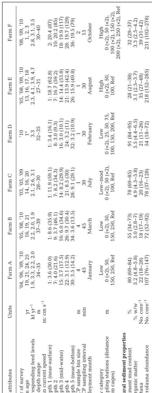
We used data obtained from an annual compliance monitoring programme over 12 yr (1998 to 2010) at 6 salmon farms located within the Marlborough Sounds, New Zealand (Fig. 1). The farms were situ-ated at comparable depths (27 to 40 m) and spanned a range of ages (1 to 25 yr of operation, Table 1). Four of these farms (A to D) had mean current velocities be-low 9 cm s−1at 20 m water depth (approximately
mid-water), and these are hereafter re ferred to as ‘non-dispersive’ sites, whereas the other 2 (E and F) had mean current velocities in excess of 15 cm s−1and are
referred to as ‘dispersive’ sites. All of the sites were situated over unconsolidated sediments; the non-dis-persive sites tended to be sandy mud (55 to 91% mud), and the dispersive sites were muddy sand (28 to 32% mud; Table 1). All of the sites had, at some point, displayed strong enrichment gradients with proximity to the farms (Keeley et al. 2012a, 2013). The analyses presented here were conducted on a deliber-ately broad range of scenarios, whereby the years that were used for each farm were selected to span a wide cross-section of total annual feed inputs and therefore presumably, associated levels of impact (Table 1).
Sediment samples were collected from directly beneath cages, and at stations along an enrichment gradient extending away from the cages (25 to 250 m), as well as at reference stations. Macrofauna were sampled using replicate (n = 2, 3 or 5, depend-ing on year of survey) Perspex sediment corers (13 cm diameter, 0.013 m2) deployed to a depth of 10
cm. Core contents were sieved to 0.5 mm, and the retained fauna was identified to the lowest practical taxonomic level and enumerated, enabling calcula-tion of a variety of community composicalcula-tion statistics and biotic indices: N (total abundance), S (number of
taxa), H’ (Shannon-Wiener diversity), AMBI (Borja et al. 2000) and BQI (Rosenberg et al. 2004). The sur-face 3 cm of smaller sediment cores (7 cm diameter) was collected for analysis of grain size and total organic matter (OM). Sediments were oven-dried to constant weight at 105°C, and size class fractions from silt-clay through to gravel were analysed gravi-metrically. Percentage OM (%OM) was calculated as the % weight loss of dried samples after ashing at 550°C for 2 h (modified after Luczak et al. 1997). Redox potential (EhNEH, mV) and total free sulphide
(TFS, µM) were also routinely measured after 2008. Re dox was measured directly from the grab (at 1 cm depth) using a Thermo Scientific combination Redox/ ORP electrode. TFS was sampled with a cut-off 5 cm3
plastic syringe driven vertically into the surface sedi-ments (0−4.5 cm depth interval), and the TFS con-tents were extracted and quantified following the methods of Wildish et al. (1999).
Bathymetry and hydrography
Bathymetry was established for each site, and the xyzdata were gridded to the desired size and
[image:3.612.307.543.398.692.2]tion using Surfer v9 for incorporation into DEPOMOD. Model grid sizes were set such that they would comfortably encompass the whole initial depositional footprint (grid areas ranged from 0.23 km2for Farm C to 1.1 km2 for Farm A).
Water currents were measured using Acoustic Doppler Current Profilers (ADCP, Sontek, 500 kHz) every 15, 30 or 45 min intervals over 25 to 42 d. ADCPs were bottom-mounted within approxi-mately 30 m from the cage edge and sampled the water column in 2 or 3 m depth bins (with a 1 m blanking dis-tance). Water current data were con-verted to hourly averaged bins, and the 5 depth bins that evenly spanned the full water column at each site (i.e. from near surface to near bottom) were selected for use in the models (Table 1).
Model parameters
DEPOMOD was selected because it is widely used and published, and was designed specifically for managing fish farm wastes (Cromey et al. 1998, Thet-meyer et al. 2003, Cromey & Black 2005, Cook et al. 2006, Magill et al. 2006); moreover, a number of the processes in DEPOMOD have already been validated against field measurements (Cromey et al. 2002a, Chamberlain & Stucchi 2007). It is also used as a regulatory tool in Scotland for discharge consents of in-feed chemotherapeutants, and in setting biomass limits (SEPA 2005), and it is the model that is recommended for predict-ing sea bed effects by the Aquaculture Stewardship Council (ASC 2012).
Standard feed wastage (Fwasted) of 3%
was used for all sites and all years in the absence of any reliable historical esti -mations. This level was selected be cause it represents a compromise between the level of 5% shown to support predictions in other studies (Cromey et al. 2009, 2012), and the level most recently deter-mined in local studies (<1%, Cairney & Morrisey 2011). Three percent is also the level currently recommended by the Scottish Environmental Protection Agency
Site attributes Units Far m A Far m B Far m C Far m D Far m E Far m F Y
ear of sur
vey
‘04, ‘06, ’09, ’10
‘05, ‘08, ‘10
‘03, ‘05, ‘09
’10
‘05, ’08, ‘09, ‘10
‘08, ‘09, ‘10
Far
m age
yr
19, 21, 24, 25
16, 19, 21
14, 16, 20
1
a
13, 16, 17, 18
1, 2, 3
Cor
responding feed levels
kt yr
−1
1.9, 3.3, 2.2, 2.0
2.2, 2.0, 1.9
2.1, 2.6, 3.1
3.3
2.3, 4.1, 3.9, 4.7
2.8, 3.1, 3.5
Site depth range
m 34−35 37−39 28−30 32−35 27−31 30−40 Mean cur rent speed
m: cm s
−1
Depth 1 (near
-sur
face)
1: 3.6 (30.0)
1: 8.6 (35.9)
1: 11.9 (59.1)
1: 3.4 (16.1)
1: 18.7 (62.8)
2: 20.4 (87)
Depth 2
7: 4.0 (21.6)
9: 3.7 (46.1)
7: 8.2 (34.3)
8: 3.0 (9.3)
7: 16.7 (59.2)
10: 20.2 (85)
Depth 3 (mid-water)
15: 3.7 (17.5)
16: 6.0 (34.6)
14: 8.2 (29.9)
16: 3.0 (10.1)
14: 14.4 (53.8)
18: 19.9 (117)
Depth 4
22: 3.1 (12.9)
26: 9.7 (30.4)
21: 8.5 (30)
24: 3.2 (11)
21: 13.9 (42.4)
28: 19.7 (129)
Depth 5 (near
-bottom)
30: 3.5 (14.2)
34: 3.6 (13.5)
28: 9.1 (29.1)
32: 3.2 (10.9)
26: 15.9 (49.8)
36: 19.5 (79)
ADCP sample bin size
m 4 4 1 1 1 2
ADCP sampling inter
val min 45 45 30 30 30 15 Deployment month Januar y M ar ch July Febr uar y August October Flow categor y Low Low Low−mod Low High High
Sampling stations (distance
m
0 (×2), 50,
0 (×2), 50,
0 (×2), 50 (×2),
0 (×2), 25, 50, 75,
0 (×2), 50,
0 (×2), 50 (×2),
fr
om cages)
150, 250, Ref
150, 250, Ref
100, Ref
100, 150, 200, Ref
100, Ref
100 (×2), 150 (×2),
200 (×2), 250 (×2), Ref
Natural sediment pr
oper
ties
Sediment mud content
% 80 (69−84) 55 (34−73) 78 (69−85) 91 (84−95) 28 (21−38) 32 (29−37) %Or ganic matter % w/w 5.2 (4.8−5.8) 5.0 (2.8−7) 4.9 (4.5−5.8) 5.5 (4.4−6.5) 3.1 (2.5−3.7) 3.3 (2.5−4.2) No. taxa No. cor e −1 22 (18−28) 18 (17−19) 20 (16−23) 21 (11−26) 35 (27−48) 39 (31−42) Macr ofauna abundance No. cor e −1 107 (76−147) 72 (52−92) 78 (37−128) 54 (18−72) 218 (152−285) 231 (102−278) aFar
m had been r
einstated for 1 yr at time of monitoring after 8 yr of r
ecovering since being fallowed in 2001
T
able 1. Summar
y of far
m configurations, historical use and physical attributes used in models, and of natural (r
efer
ence site,
Ref) sediment characteristics for each site.
Cur
rent speeds for each depth bin (in m; left of colon) ar
e mean values, with maximum speed in brackets. For sampling stations,
‘×2’ denotes 2 separate sampling stations
for the given position. Sediment pr
oper
ties show mean values and ranges (min−max) fr
om the r
efer
ence sites that wer
e sampled du
ring the selected sur
veys for each far
m.
ADCP: Acoustic Doppler Cur
rent Pr
[image:4.612.91.338.82.718.2](SEPA) for regulatory modelling of fish farms in Scot-land (Annex H in SEPA 2005). Feed digestibility (Fdig)
and water content (Fw) were set at 85 and 9%,
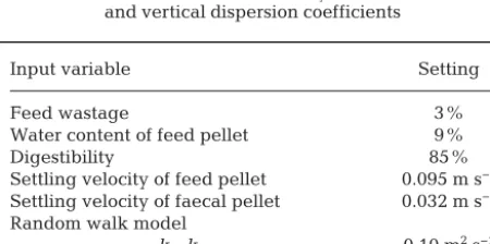
respectively, which are the DEPOMOD defaults based on technical data provided by feed manufac-turers (Cromey et al. 2012) and were used in the absence of farm and time-specific estimates. All other model parameters were consistent with exist-ing salmon farm waste modellexist-ing methodologies (Cromey et al. 2002a,b) and the SEPA Annex H reg-ulatory farm modelling standards (SEPA 2005), and remained constant in the tested model scenarios (Table 2). As the model does not allow the settling velocity of particles to change through the growing cycle, the values used for feed and faeces repre-sented those that would be encountered during the period of highest waste output from the farm (maxi-mum standing biomass), which is when the fish are at pre-harvest size.
Feed input data were based on total feed used per farm per month and spread evenly across all cages. In practice, 1 or 2 cages may be empty for short periods of time as a result of operational require-ments, but this resolution of spatial and temporal information was not available and would be imprac-tical to include in the model. However, this repre-sents a potential source of variability in the outputs, which was accounted for by taking the average result from multiple scenarios. The farm manage-ment conditions for each scenario (i.e. number of cages, net depths, overall size and position of farm and monitoring stations) were determined from information collected during annual monitor-ing surveys (e.g. GPS fixes of farm corners), histori-cal aerial and satellite images, and discussions with farm operators. The standard farm configurations involved square cages with a net depth of 20 m arranged in adjoining clusters, either 1 or 2 cages wide and 4 to 8 cages long.
Depositional flux was predicted for 110 benthic sampling locations, representing 18 different histori-cal farming arrangements, encompassing all 6 study farms (Farms A to F) over 8 yr (2003 to 2010, Table 1). Results were obtained for 4 different feed levels based on the average reported feed use for the 1, 3, 6 and 12 mo immediately prior to the environmental data being collected. Four critical resuspension ve -locities were contrasted within each average feed use period: (1) without resuspension, or with resus-pension based on critical velocity thresholds (vr) of: (2) 9.5 cm s−1(model default), (3) 12 cm s−1and (4)
15 cm s−1. Thus, 16 model runs were conducted for
each of the 18 different farming scenarios, giving a total of 288 runs. Matlab™ code was developed to enable batch processing of model runs.
Relating predicted flux to observed enrichment stage
Environmental condition was determined using established ecological indicators: N, S, H’, AMBI and BQI in combination with physico-chemical variables (%OM, redox, TFS). All variables were also unified following the methods of Keeley et al. (2012a,b) to obtain an indication of overall enrichment stage (ES), a bounded continuous variable that places the results on a scale between ES1 = ‘pristine’ to ES7 = azoic/ anoxic. Generalised additive modelling was then used to establish the relationship between predicted flux and observed ecological responses, as shown by ES and each the individual indicator variables.
Prior to analysis, both predicted flux and ES values were log-transformed to improve data normality and reduce heteroscedasticity. The necessity to construct flow-specific models was checked by testing the significance of Flow as a fixed factor (high/low) using linear models in R (R Development Core Team 2011). In all cases, Flow was highly significant (p < 0.0001). The optimum linear model was then identi-fied by fitting 4 different polynomials (of order 1 to 4) and then selecting the model with the smallest Akaike Information Criterion (AIC) value. If the AIC values of 2 models were within 2 units (and could therefore be considered equivalent, Burnham & Anderson 2002), then the simplest model was chosen in preference. The best-fit polynomials were solved for x(or ES) to obtain estimates of the average flux associated with ES3 (i.e. ES = 3) and ES5 (i.e. ES = 5), and the standard errors of the coefficients were used to calculate the associated 95% pointwise confidence bounds (hereafter referred to as confidence intervals, CI). ES3 was selected to represent the outer
bound-Input variable Setting
Feed wastage 3%
Water content of feed pellet 9%
Digestibility 85%
Settling velocity of feed pellet 0.095 m s−1 Settling velocity of faecal pellet 0.032 m s−1 Random walk model
kx, ky 0.10 m2s−1
[image:5.612.62.287.608.720.2]kz 0.001 m2s−1
Table 2. Default model settings that were applied consis-tently throughout the modelling. kx, kyand kzare horizontal
ary of effects be cause this level is considered indicative of the point at which enrichment becomes clearly discernible, whilst ES5 indi-cates the point of peak infauna abundance, and characterises a highly enriched state (Keeley et al. 2012a).
Model validation: spatial comparison of predicted and observed footprints
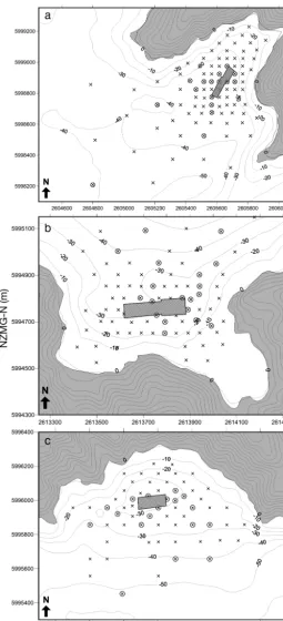
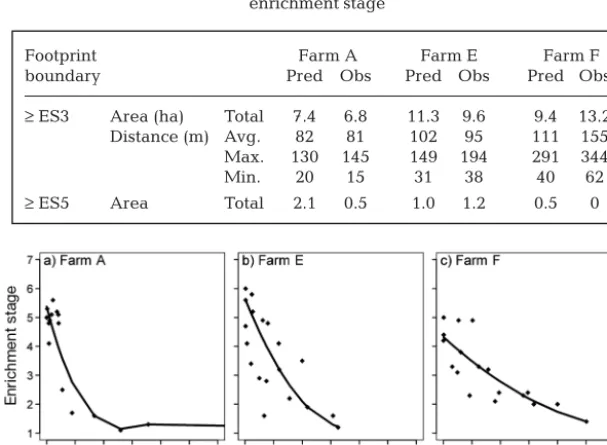
The footprints of the 2 high-flow, dispersive farms (Farms E and F) and 1 low flow, non-dispersive farm (Farm A) were mapped from 79, 65 and 96 grab sampling stations (respectively) collected across a grid pattern spanning the sediments within 1.5 km of the cages. In all cases, the density of the sampling grid decreased with distance from the farm in a stratified manner to ensure that sampling effort was greatest where changes in the footprint were expected to be most pronounced (Fig. 2). These farms were se -lected because they had similar farm layouts, and they had consistent usage patterns (cage deploy-ment and feed input) in recent years. They also share similar physical attributes (i.e. depths and exposure), but vary significantly in their typical range of current speeds (Table 1). We were only able to survey 3 farms because of logistical and financial constraints.
Enrichment was assessed at all sampling sta-tions using 3 proxy variables: (1) sediment redox (EhNHE, mV), (2) sulphide (S2−, µM) levels and (3)
[image:6.612.286.542.81.643.2]odour. Odour was assessed consistently by the same person using 5 categories: 1 = none, 2 = mild, 3 = moderate, 4 = strong, 5 = very strong. Approximately 20 stations at each farm, repre-senting the full range of conditions (i.e. from alongside cages to the most distant reference site) were selected for more comprehensive con-dition assessments, comprising macrofauna eval-uation, sediment grain size characterisation and %OM content following the methods described above. The 3 proxy variables were combined multi variately using principle component analy-sis (PCA, in PRIMER v5, Clarke & Gorley 2006) based on Euclidean distances. Sulphide and re -dox data were log-transformed, and all variables were normalised prior to analysis. The eigen -values of the dominant PCA axis were used to quantitatively differentiate the sampling stations. ES was also determined for each of the compre-hensively sampled stations using a combination
Fig. 2. Sampling grids that were used to map the enrichment footprints at the 2 high-flow study sites, Farms A (a), E (b) and F (c). ×: stations where the 3 proxy variables (redox, sulphide, odour) were sampled; ⊗: stations with comprehensive sampling (including macrofauna, sediment grain size and % organic matter). Grey box denotes position of net pens. Axis units are in metres — east and
of the empirical relationships derived by Keeley et al. (2012a) and best professional judgement.
The linear regression that best de scribed the relationship (based on highest residual R2values) be tween the eigen values (based
on redox, sulphides and odour) and the ES score was determined for each farm sur-vey. These regressions were then used to estimate ES for all stations based on the eigenvalues, and the results interpolated using the Kriging method (Isaaks & Srivas-tava 1989) before being spatially depicted in Surfer™ (v9). Finally, the measured print was compared to the predicted foot-print by converting the predicted flux for the corresponding farm scenario to ES using the best-fit relationships that were identified from modelling the historical farming scenarios. ES3 was selected to in -dicate the outer boundary of effects for the reasons given in the previous subsection.
RESULTS
Relating predicted fluxes to observed ecological responses
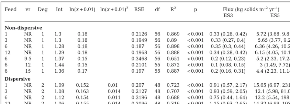
The central tendency of the relationships between observed ecological re sponses (as indicated by ES) and the predicted deposi-tional flux (as the explanatory variable), without resuspension, was best described by first- and second-order polynomials on log-transformed data (Fig. 3, Table 3). The best model fit for the non-dispersive sites was obtained with the feed levels applied over the 6 mo preceding the respective sampling events (R2= 0.898). However, the
differences between the 4 time series scenarios (i.e. 1, 3, 6 and 12 mo prior), were small, with R2values of
between 0.869 and 0.890 (Fig. 3a−d, Table 3). A mod-erate/detectable level of enrichment (i.e. ES3) was associated with an average predicted flux of between 0.33 (CI: 0.27, 0.4) and 0.35 (CI: 0.3, 0.44) kg solids m−2yr−1. Very highly enriched conditions, indicative of peak macrofauna abundance (i.e. ES5), were asso-ciated with modelled depositional fluxes of between 5.6 (CI: 3.7, 9.2) and 6.3 (CI: 4.2, 10.6) kg solids m−2
yr−1(Table 3).
The model fits for the dispersive sites without resuspension had slightly lower R2 values than for
the non-dispersive sites, with results for the 4 feed levels ranging between 0.73 and 0.78 (Fig. 3a−d, Table 3). The modelled fluxes associated with ES3-type conditions at the dispersive sites were higher than at the non-dispersive sites, with fluxes ranging between 0.75 (CI: 0.44, 1.64) and 1.15 (CI: 0.67, 2.65) kg solids m−2 yr−1 (Table 3). Similarly, the average predicted flux associated with ES5-type conditions was approximately 2-fold higher for dispersive sites than for the non-dispersive sites, with estimates of between 12.1 (CI: 5.9, 81.1) and 15.6 (CI: 6.9, 231) kg solids m−2yr−1. However, the upper confidence
inter-vals for these estimates were very high due to in -Fig. 3. Log–log relationships for predicted depositional flux and observed enrichment responses (as the response variable) at sampling stations associated with 4 low-flow (Farms A–D) and 2 high-flow farms (Farms E and F). Equations and model fit parameters are provided in Table 3. Thin dashed lines show 95% pointwise confidence bounds for the fitted curves. NR: no resuspension, vr: critical resuspension threshold used,
[image:7.612.255.537.82.480.2]creased variation at the upper end of the enrichment gradient and the log-relationship between flux and ES. Where resuspension was taken into account (Fig. 3e−g), the model outputs were comparable with the no-resuspension results for non-dispersive sites. Although the overall fit with the observed data was worse, this improved from R2= 0.65 to 0.88 as the
crit-ical resuspension velocity increased from 9.5 cm s−1
(model default) to 15 cm s−1. The poorer fit when
resuspension was included in the scenario was pri-marily due to the predicted fluxes for some of the moderately enriched stations (i.e. ES3−5) at Farm C (which has the highest current speed of the 2 non-dispersive sites) being 0. At the non-dispersive sites, the net depositional flux was predicted to be 0 for all 3 critical resuspension velocities, even at stations that were directly beneath the cages. As a result, no meaningful relationship could be derived between flux and effects for those scenarios.
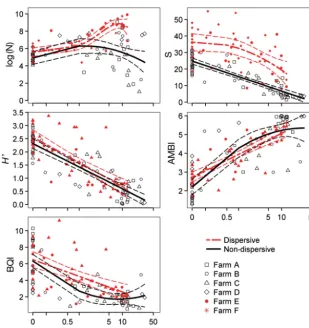
The relationships between predicted depositional flux and individual response variables were gener-ally not as strong as the relationships with the multi-variable derived ES (Fig. 4). However, H’ and AMBI were both reasonably well predicted by the models at both dispersive and non-dispersive sites (R2= 0.56 to 0.76, Table 4). Number of taxa (S) and BQI were poorly predicted by depositional flux at the dispersive sites (R2= 0.27 and 0.31, respectively), but
well predicted at the non-dispersive sites (R2 = 0.78
and 0.56, respectively). Conversely, log(N) was re -lated to predicted flux at the dispersive sites (R2 =
0.65), but not at the non-dispersive sites (R2 = 0.07);
the former was best described by a more complex fourth-order polynomial.
Model validation: spatial comparison of predicted and observed footprints
The primary axis of the PCA analysis (i.e. PC1), integrating the 3 proxy variables (redox, S2− and
odour) was a good indicator of the overall variation between stations at Farms E and F (N = 64 and 84, variation described by PC1 = 84 and 85%, respec-tively). The resulting PC1 values also correlated well with the ES scores determined from the 18 to 19 samples for which infauna and %OM information was also collected (R2= 0.58 to 0.81, Table 5). PC1 for
Farm A (N = 90) captured slightly less of the overall variability (61%) than for Farms E and F, but still cor-related well with ES (R2= 0.808). Hence, the
relation-ships were considered adequate for converting the PC1 scores from the wider survey into an estimated ES value for each farm site. The predicted deposi-tional flux for each of the farms was also converted into the same ES variable to enable direct compari -sons, using the best relationships identified in Table 3. The predicted area of enrichment at ES3 or greater was comparable to the observed footprints. The size of the predicted footprint at ES3 was 11.3 and 9.4 ha for Farms E and F, which compares favourably with the observed footprint 9.6 and 13.2 ha (respectively). Feed vr Deg Int ln(x+ 0.01) ln(x+ 0.01)2 RSE df R2 p Flux (kg solids m–2yr–1)
ES3 ES5
Non-dispersive
1 NR 1 1.3 0.18 0.2126 56 0.869 < 0.001 0.33 (0.28, 0.42) 5.72 (3.68, 9.81) 3 NR 1 1.3 0.18 0.1949 56 0.89 < 0.001 0.33 (0.27, 0.4) 5.65 (3.77, 9.2) 6 NR 1 1.28 0.18 0.187 56 0.898 < 0.001 0.35 (0.3, 0.44) 6.36 (4.26, 10.26) 12 NR 1 1.29 0.18 0.1968 56 0.888 < 0.001 0.34 (0.28, 0.42) 6.15 (4.05, 10.19) 6 9.5 1 1.37 0.15 0.3468 56 0.651 < 0.001 0.2 (0.12, 0.23) 5.2 (2.33, 17.25) 6 12 1 1.44 0.15 0.2101 55 0.872 < 0.001 0.1 (0.08, 0.15) 3 (1.49, 7.72) 6 15 1 1.36 0.17 0.197 55 0.887 < 0.001 0.2 (0.16, 0.31) 4.4 (2.23, 11.18)
Dispersive
[image:8.612.59.536.161.332.2]1 NR 2 1.09 0.152 0.01 0.207 48 0.723 < 0.001 0.91 (0.57, 2.17) 15.65 (6.97, 231.9) 3 NR 2 1.08 0.163 0.014 0.2127 48 0.707 < 0.001 0.93 (0.59, 2.05) 12.1 (5.98, 81.07) 6 NR 2 1.12 0.154 0.011 0.2196 48 0.688 < 0.001 0.75 (0.44, 1.64) 12.2 (5.54, 198.5) 12 NR 2 1.06 0.155 0.014 0.2096 48 0.716 < 0.001 1.15 (0.67, 2.65) 14.72 (6.99, 103.5) Table 3. Summary of polynomial coefficients and fits for relationships between predicted depositional flux and observed en-richment stage (ES, as the response variable). Average flux (kg solids m−2yr−1) required to induce ES3 (moderate, detectable enrichment) and ES5 (very high enrichment defined by peak of opportunistic taxa) provided along with upper and lower con-fidence interval (CI, in brackets). Feed: period preceding field sampling over which feed use was averaged, vr: critical velocity for resuspension (cm s−1), NR: no resuspension, Deg: degree of polynomial, Int: intercept, RSE: residual standard error. Note that no meaningful relationship could be derived between flux and effects for results from dispersive sites with resuspension
The average total distance to the outer extent of ES3 conditions was also comparable, 102 m (predicted) and 95 m (observed) for Farm E, and 111 m (pre-dicted) and 155 m (observed) for Farm F (Table 6). Both the modelled and the predicted scenarios for the dispersive farms show a generally lower and more
diffuse level of enrichment. Farm F had the widest footprint but did not exceed ES ~4.5 anywhere. These patterns are summarised in Fig. 5a−c, which illus-trates how the spatial extent increases and the impact decreases from Farm F > Farm E > Farm A.
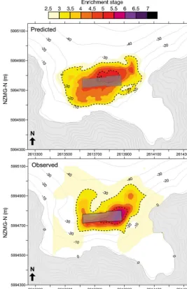
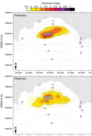
[image:9.612.45.355.80.409.2]The shape and intensity of the foot-prints at the dispersive sites were also reasonably well predicted by the model (Figs. 6 & 7). Both the model and obser-vational data show an im pacted region (ES > 5) to the north-east of Farm E (Fig. 6); the extension of the footprint to the north-east and north-west was also evident in the model output. However, the degree of impact was slightly under-predicted by the model and the associ-ated ES score. The predicted footprint for Farm E was also slightly wider than the actual footprint through the centre. The observed footprint for Farm F was larger and more diffuse than pre-dicted, with low level effects extending farther to the south (toward the main channel) and west (Fig. 7). Not ably the model predicted very intense effects directly beneath Farm F which were not observed. However, overall the agree-ment between the observed and pre-dicted footprints for Farm F was good. The agreement between the overall size of the ob -served and predicted footprints for the non-dispersive Farm A was also good (Fig. 8). Differences on the whole were minor and mostly related to slight changes in the footprint outline. The predicted scenario had a slightly larger highly impacted area Fig. 4. Relationships between predicted (log) depositional flux and 5
enrich-ment indicators of biological variables. Line details as in Fig. 3, equations and model fits are provided in Table 4
Variable Deg Int x x2 x3 x4 RSE df R2 p
Non−dispersive log(N) 2 5.41 1.1 −3.99 1.642 55 0.071 0.049
S 1 14.65 −63.96 4.478 56 0.780 < 0.001
H’ 1 1.35 −6.05 0.418 56 0.762 < 0.001
AMBI 2 3.97 10.06 −1.93 0.924 55 0.679 < 0.001
BQI 2 3.59 −14.81 4.8 1.789 55 0.564 < 0.001
Dispersive log(N) 4 6.86 8.06 1.91 −0.32 −2.1 0.861 46 0.654 < 0.001
S 2 30.72 −42.51 −15.06 9.824 48 0.276 < 0.001
H’ 1 1.69 −4.94 0.613 49 0.561 < 0.001
AMBI 1 3.82 6.14 0.600 49 0.674 < 0.001
BQI 1 4.69 −10.28 2.113 49 0.311 < 0.001
[image:9.612.63.537.584.721.2](ES > 5) directly beneath the cages, and the southern (seaward) end of the observed footprint was slightly less impacted than predicted.
DISCUSSION
Predicting effects at dispersive sites
The log relationship identified between predicted flux and ES is due to large increases in enrichment in response to small increases in depositional flux over the first part of the enrichment gradient (ES1−3). Over the latter part of the enrichment gradient
(ES5−7), large flux increases were associated with relatively small changes in ES. This reflects both the sensitivity to, and scope for, ecological change with the addition of organic biodeposits; this suggests that ‘natural’ sediments will respond noticeably to small (persistent) additions of organic material, but that when sediments are already impacted, significant additions may be necessary to affect a relatively small change in enrichment stage. There are a num-ber of possible explanations for this result. Firstly, it may be an artefact of the overall scale of change over the respective parts of the enrichment gradient (e.g. ES6 and ES7 versus ES2 and ES3) and/or may high-light a relative insensitivity to changes in the higher enrichment stages. Alternatively, it may reflect the fact that the impact gradient is bounded and that conditions cannot get appreciably worse than those indicated by ~ES6.5, and therefore there is limited scope for further degradation with any additional feed inputs. The most likely scenario is a combination of these 2 mechanisms, whereby the degree of change indicated by the macrofauna-related variables at that end of the spectrum is limited (Keeley et al. 2012a) and bounds our present understanding as to the limits of effects. The additional capacity is presum-ably facilitated by the seabed progressing from an as similative phase, where the macro-fauna are prolific, to a state of organic accumulation, dominated by micro-bial processes and where changes may be better defined by other physico-chemical variables.
When the process of resuspension was modelled at the 2 dispersive sites, predictions indicated that all particles would be exported, irrespective of the critical resuspension velocity used (i.e. vr = 9.5, 12 or 15 cm s−1).
Accord-ing to the conventionally held view that benthic effects are proportional to depositional flux (Cromey et al. 2002a), the resultant effects would be negligible — but this was not the case. There was minimal evidence of organic accumulation (indicated by %OM); however, pronounced ecolog-ical effects were identified at both dis-persive sites. A similar observation was made by Chamberlain & Stucchi (2007) at a moderately dispersive site in Canada, where DEPOMOD pre-dicted that virtually all of the material would be exported from the site, yet
Farm Equation R2 N
A y= exp(0.348x) × 2.14 0.808 17
E y= 0.625x+ 3.125 0.720 19
[image:10.612.58.287.151.212.2]F y= 0.651x+ 2.899 0.581 18
Table 5. Best-fit linear models of PC1 in relation to enrich-ment stage (ES) derived from the subset of stations that were more comprehensively sampled (ES determined from em-pirical relationships with sulphide [S2−], redox, % organic matter, total abundance, no. taxa, AMBI and BQI [see ‘Mate-rials and methods’]; PC1 determined from redox, S2−, odour)
Footprint Farm A Farm E Farm F boundary Pred Obs Pred Obs Pred Obs
≥ES3 Area (ha) Total 7.4 6.8 11.3 9.6 9.4 13.2 Distance (m) Avg. 82 81 102 95 111 155 Max. 130 145 149 194 291 344 Min. 20 15 31 38 40 62
[image:10.612.54.358.456.679.2]≥ES5 Area Total 2.1 0.5 1.0 1.2 0.5 0 Table 6. Dimensions of predicted (Pred) and observed (Obs) footprints asso -ciated with 1 low-flow farm (Fig. 8) and 2 high-flows (Figs. 6 & 7). Predicted footprints are based on 2010 site configurations and farming intensities. ES:
enrichment stage
localised seabed enrichment was evident. This sug-gests that either the resuspension component of the model is overpredicting how much material is being exported, or the model is correct and the popular understanding of how ecological effects are induced at dispersive sites is incomplete.
Overprediction of particle advection by the model may occur where the critical resuspension velocity (vr) is set too low, or where the numerical algorithms describing resuspension do not consistently
repre-sent the key dynamical processes. Chamberlain & Stucchi (2007) suggested that the default vr in DEPOMOD (9.5 cm s−1, previously ‘hard-coded’
into the model) may indeed be too low, but also that using a single value was probably too simplistic, given the difference between the vr required to suspend feed pellets compared with fish faeces. The current study showed that observed effects occurred in conjunction with a predicted flux of 0 when a vr of 9.5 cm s−1was
used, but that this disparity decreased as vr was increased toward 15 cm s−1— thereby de
-creasing predictions of total advection. By experimenting with even higher vr values at the 2 dispersive sites (model outputs not shown), it was determined that vr values in excess of 35 cm s−1 would be required in order for significant
accumulation to occur. Waste feed pellets are known to roll and saltate (bounce) at current speeds of 16 to 20 and 32 to 40 cm s−1,
respec-tively (Sutherland et al. 2006); consequently, it is likely that the resuspension of those particles was overpredicted by the model. However, at the sites in this study, waste feed was recently estimated to be <1% (Cairney & Morrisey 2011), and therefore the deposition would have com-prised mostly faecal particles, which resuspend at much lower current speeds, on the order of 7 to 15 cm s−1(Cromey et al. 2002b). Given that
the physical properties of the main bio deposits (i.e. feed pellets or faeces) would be broadly comparable irrespective of region and/or site characteristics, the vr values that would be required to achieve particle accumulation at the dispersive sites seem unrealistically high. Hence, it seems more likely that the model pre-dictions using the default vr setting are reason-ably accurate and that the observed impacts are occurring in the absence of significant organic accumulation. This effect has been described for these dispersive systems (Keeley et al. 2013) and is characterised by proliferation of oppor-tunistic taxa in the presence of an elevated carbon flux and a strong oxygen supply, but in the absence of sig nificant organic accumulation and the associated sediment anoxia, which would normally limit bio logical production (Findlay & Watling 1997, Hargrave et al. 2008).
[image:11.612.48.316.82.497.2]Although the model outputs incorporating resus-pension may be faithfully reproducing the physical processes, the results are not very useful for the pur-poses of predicting either the spatial extent or magni-tude of seabed effects at higher-flow sites. Using Fig. 6. Predicted (top) and observed (bottom) benthic
the no-resuspension scenarios to predict flow-spe-cific effects, in a similar manner to that adopted by Chamberlain & Stucchi (2007), we established sepa-rate relationships between predicted flux and overall enrichment effects (ES) for non-dispersive and dis-persive sites; the main difference was that a greater discharge was required to induce an equivalent level of effects at the dispersive sites. According to these relationships, moderate, detectable levels of enrich-ment (i.e. ES3) occur with the addition of ~0.4 kg solids m−2 yr−1 for non-dispersive sites and ~1 kg
solids m−2yr−1for dispersive sites. ES5-type impacts,
indicative of peak abundance beyond which the macrofauna is at increased risk of a collapse (ES6−7,
Keeley et al. 2012a), are induced by the addition of ~6 kg m−2 yr−1 for
non-dispersive sites and approximately double that amount for dispersive sites (i.e. ~13 kg m−2yr−1). The difference between these 2
thresh olds (i.e. ~5 kg m−2 yr−1 or ~50%),
which compare favourably with previous attempts to link depositional flux to en -richment response (Table 7), may be related to the amount of material that is being exported from the immediate vicin-ity, over and above what is either settling (and being buried) or being biologically assimilated locally.
A flux rate, over and above natural background sedimentation, of around 1 to 1.5 kg m−2yr−1has been identified in
sev-eral previous studies as the point at which clear changes in the macrofauna commu-nity and/or the oxic status of soft sedi-ments may be observed (Hargrave 1994, Findlay & Watling 1997, Cromey et al. 2002a, 2012, Chamberlain & Stucchi 2007). These estimates are slightly higher than those identified for ES3 at non-dispersive sites in the present study (i.e. ~0.4 kg m−2
yr−1). However, it is difficult to determine the exact level of enrichment referred to in each case due to the differing suites of individual indicators and threshold descrip -tions that are employed. Accordingly, it is possible that the enrichment level (ES3) used in the present study, based on multi-ple indicators, represents a more sensitive threshold. The particular ecosystem effect to be assessed may also influence the re -quired sensitivity of the measured response. For instance, Holmer et al. (2008) iden -tified a similar flux (0.5 kg m−2 yr−1) as
the point beyond which seagrass shoot mortality was accelerated, whilst the suggested threshold for effects to more sensitive maerl bed communities would appear to be appreciably lower at 0.1 kg m−2
yr−1(Sanz-Lázaro et al. 2011). Cromey et al. (2002a)
associated the peak in opportunistic taxa, which equates to ES5-type conditions, with a depositional flux of 10 kg m−2yr−1for non-dispersive sites, which is double that proposed for comparable flow regimes in this study (4 to 5 kg solids m−2yr−1) and still less
[image:12.612.43.343.80.523.2](i.e. feed waste presumably has higher enrichment potential than faecal waste, Chamberlain & Stucchi 2007).
For the purposes of this study, sites were cate-gorised as being either dispersive or non-dispersive based on their current speeds and how these relate to the vr of 9.5 cm s−1. Sites with near-bottom speeds above vr greater than 50% of the time were treated as ‘dispersive’; this categorisation was both concep-tually logical and consistent with observations of how the seabed effects manifested at the sites over the previous 10 yr. Sites with ‘intermediate’ physical properties (central to this threshold), or with notably
higher current speeds, may require spe-cial consideration (e.g. use of an alterna-tive flux−ES relationship).
Relationships between predicted flux and individual indicator variables were generally weaker than those with ES, which integrates multiple biotic and abi-otic variables. Of the individual indicators, AMBI appeared most versatile, relating to flux at both non-dispersive and dispersive sites. This result is not surprising given that the AMBI is considered to be a good predictor of overall enrichment state (Keeley et al. 2012a). Macrofauna abun-dance (N) was particularly poorly pre-dicted by flux at non-dispersive sites, being highly variable when flux was elevated. However, there was a notable spike in N at both the dispersive and non-dispersive sites at around 10 kg m−2yr−1,
which aligns reasonably well with both the position of the abundance and bio-mass peaks identified by Cromey et al. (2012), and ES5 conditions, as de scribed above. Species richness (S) was strongly negatively correlated with flux at the non-dispersive sites, which was consistent with Cromey et al. (2012), who observed a relatively consistent decline below ~0.1 kg m−2yr−1. S showed a relatively poor
rela-tionship with flux at the dispersive sites, presumably because high flow environ-ments tend to be more resilient to de position (Keeley et al. 2013). This obser -vation is symptomatic of the processes discussed above, whereby the seabed en -counters high levels of depositional flux, but as much of it is exported, accumula-tion and the associated physico-chemical effects are limited.
[image:13.612.44.344.83.542.2]alterations to the overall size or shape of the foot-print; however, this would only result if the loss from erosion at the outer margin of effects, and from parti-cles going into solution and being assimilated by the environment, is less than the load that is being re -distributed. This process was encompassed to some extent in this study, as most of the sites have been consistently utilised for many (> 5) years and there-fore should be in a relatively stable state.
Using the primary footprint to gauge the extent of the ‘main effects’ for new or proposed sites can pro-vide useful guidance for setting initial farm manage-ment objectives (e.g. allowable zone of effects, AZE). The present ASC standards (ASC 2012) for the AZE for salmon farming permit a relatively modified state, whilst the discussion provided above considers less obvious potential effects beyond that zone. Effects in the outer regions will be inherently subtle and diffi-cult to definitively distinguish from ‘natural’ change. Consequently, delineating a more accurate ‘impacts’ boundary will always be challenging and fraught with subjectivity.
Using shorter feed time series made very little difference to the robustness of the relationships be -tween predicted and observed effects, suggesting that there is little to be gained in terms of resolving tempo-ral dynamics in enrichment effects from using higher temporal resolution feed information, especially with-out finer resolution, cage-scale stocking/ feed use information. Therefore, using the average feed con-sumption information for the medium-term (ca. 3 or
6 mo) period preceding the required benthic evalua-tion appears to be adequate for predicting effects.
In both the dispersive and non-dispersive exam-ples, there was some scatter about the data. This may in part be related to minor inaccuracies with recreat-ing the spatial arrangements in the models (i.e. posi-tioning the sample stations in relation to the farms), and/or the inability to accurately recreate historical farming conditions. For example, it was not possible to include within-farm stocking variations (i.e. tem-porarily empty nets and fish rotation). Additionally, the application of a constant waste feed value (which has a strong influence on flux estimates, Chamber-lain & Stucchi 2007) was probably overly simplistic as improvements in feeding techniques are likely to have reduced wastage over the study period. Finally, some of the scatter may also be due to natural spatial and temporal varia bility in the benthos (e.g. Thrush 1991), which in turn may be more pronounced under highly enriched conditions. Nevertheless, the errors presumably operated in both directions (over- and underestimation), and the measures of the central tendency described should remain valid.
Spatial comparison of predicted and observed footprints
Overall, the predicted footprints using the no-resuspension scenarios corresponded well to the observed footprint in terms of size, shape and overall Depositional flux Associated ecological threshold/conditions Source
gC m−2d−1 kg solids m−2yr−1
0.28 0.35 Non-dispersive sites ES3 (moderate/detectable
This study (average values) 0.76 0.93 Dispersive sites enrichment)
4.9 5.9 Non-dispersive sites ES5 (highly enriched) This study (average values)
11.2 13.6 Dispersive sites
1.7 2.1 Enriched seabed beneath blue mussel farms Dahlbäck & Gunnarsson (1981) 1 1.2 Formation of hypoxic sediments around salmon farms Hargrave (1994)
1 to 5 1.2 to 6.1 Threshold at which macrofauna biodiversity is reduced Findlay & Watling (1997) by salmon biodeposits
0.01 0.01 Macrofauna change begins based on infaunal trophic Cromey et al. (2002a) index
0.82 1 Significant change in composition Cromey et al. (2002a)
8.22 10 Corresponds to peak in opportunists Cromey et al. (2002a)
1 to 5 1.2 to 6.1 Significant change in macrofauna community (also Chamberlain & Stucchi (2007) transition between oxic/healthy and anoxic/degraded
benthic zonation status)
> 4.5 > 5.5 Significant alterations to the benthic community beneath Weise et al. (2009) mussel farms
0.087 0.1 To maintain diversity of maerl beds Sanz-Lázaro et al. (2011) 1.23 1.50 Boundary beyond which clear pollution indicative Cromey et al. (2012)
[image:14.612.57.539.99.336.2]changes occur in macrofauna
Table 7. Summary of proposed depositional flux thresholds and the associated benthic enrichment effects. ES: enrichment stage
intensity. Hence, the use of non-resuspension scenar-ios to predict the effects at dispersive sites appears valid, particularly when ES3, indicative of moder-ate/detectable enrichment, is used to delineate the outer extent of effects. The ES3 threshold was se lected because it clearly indicates anthropogenic en -richment; ES levels < 3 can occur naturally (Keeley et al. 2012a). Using thresholds <ES3 increases the risk of including areas that are not necessarily en riched as a result of farm activities in the footprint. ES≥3.0 is therefore recommended as a useful limit for delineat-ing farm effects boundaries unless there are good grounds to justify a lower threshold, i.e. comprehen-sive baseline information.
Agreement between the predicted and observed footprints declined in the more severely impacted regions (i.e. directly beneath the cages), possibly due to the lack of observational data from directly beneath the cages and/or to an overestimation of feed wastage. Although severe impacts might be expected at non-dispersive sites, they would be less likely at dispersive sites where strong currents can diffuse the intensity of impact. A recent study con-ducted at Farm F showed that feed wastage was <1% (Cairney & Morrisey 2011). The modelling in the present study was conducted with a feed waste of 3% for the reasons outlined in the
‘Materials and methods’. Chamberlain & Stucchi (2007) suggested that waste feed is responsible for the majority (i.e. 70% at 5% waste) of the carbon flux beneath the cages and as far as 60 m away, but beyond that the contribu-tion is dominated by the smaller and more slowly settling faecal particles. Therefore, if the farms can achieve near-0 feed wastage, then the impacts under and near the cages may be re -duced. The effect of using a 1% waste feed level was tested for Farm F, with the results indicating that the footprint (ES > 3) was a similar shape and size (0.2% smaller), but that the area of seabed predicted to be impacted to ES > 5 was slightly smaller (by 0.26 ha, or 2.3% of the footprint). As such, the effect of adjusting the waste parame-ter by 2% for the given scenarios was considered minor. In addition, some of the shape aberrations may reflect fine-scale farm use practices (e.g. periodi-cally empty nets within farms and/or any temporary extensions or
contrac-tions of farms) or hydrodynamic condicontrac-tions (e.g. storm events) that were not captured by the models.
CONCLUSION
Localised benthic impacts may still be observed even where depositional models suggest otherwise, as significant benthic effects can occur in the per-ceived absence of organic ‘accumulation’. A useful indication of the spatial extent of such effects can be obtained when the model is parameterised without resuspension: this suggests that approximately twice the amount of deposition flux is required to induce effects at dispersive sites compared to non-dispersive sites. Specifically, moderately enriched conditions (ES3) were associated with ~0.4 kg m−2yr−1for
non-dispersive sites and ~1 kg m−2 yr−1 for dispersive
sites, whilst highly enriched conditions (peak infauna abundance; ES5) were associated with ~6 and ~13 kg m−2 yr−1 for nondispersive and dispersive sites, re
-spectively.
[image:15.612.239.538.409.644.2]Three main interactive ecosystem process compo-nents underpin the ultimate enrichment response (Fig. 9). At non-dispersive sites, total deposition (A) almost entirely equates to net deposition (B), which
Fig. 9. Summary of major pathways for salmon farm feed-derived bio -deposition. A: total biodeposition = all waste particulates produced by the farm (feed and faeces, ignoring dissolved organic component). B: net biodeposition includes the particulates that settle, accumulate and/or are used (as -similated) in the near-field or ‘primary footprint’. C: resuspension and advec-tion includes the fracadvec-tion of A that is exported from the immediate vicinity by
comprises B1 (settlement, consolidation and ulti-mately burial) and B2 (assimilation by benthic biota), with little or no influence from C (resuspension). In contrast, at dispersive sites, B1 is minimal and the impact is characterised by processes B2 and C1 (water column dilution and assimilation by biota) with the additional influence of far field deposition and subsequent assimilation and burial (C2); these processes together comprise the resuspension and advection process (C).
For a large footprint (i.e. dispersive sites) combined with significant sediment re suspension and advec-tion (process C) and abundant opportunistic taxa (i.e. a larger B2 component), the overall load to the eco-system (A) can be much larger: in this study, the seabed at the dispersive sites sustained twice as much particulate matter as the non-dispersive sites. Whilst the ratio between B and C was not quantified in this study, the differences between the flux re -quired to induce equivalent levels of effects at the dispersive and non-dispersive sites provides some indication of this response, i.e. ~7 kg m−2yr−1at ES5,
or ~50% of A. Understanding the empirical relation-ship between C1 and C2 is particularly important for characterising impacts at dispersive sites and would be a worthwhile area for further research.
Acknowledgements. This research was supported by the
Cawthron Institute (Nelson, New Zealand) through internal investment funding (IIF), with additional support from the Institute of Marine and Antarctic Sciences (IMAS), Univer-sity of Tasmania. We also acknowledge the support of New Zealand King Salmon Company Ltd., who allowed the research to be conducted at their farms, made available much of the source data and supported the dissemination of the findings.
LITERATURE CITED
Apostolaki ET, Tsagaraki T, Tsapakis M, Karakassis I (2007) Fish farming impact on sediments amd macrofauna asso-ciated with seagrass meadows in the Mediterranean. Estuar Coast Shelf Sci 75: 408−416
ASC (Aquaculture Stewardship Council) (2012) ASC salmon standard. Version 1.0 June 2012. Available at www.asc-aqua.org/upload/ASC%20Salmon%20Standard_v1.0.pdf Borja A, Franco J, Perez V (2000) A marine biotic index to establish the ecological quality of soft-bottom benthos within European estuarine and coastal environments. Mar Pollut Bull 40: 1100−1114
Borja A, Rodríguez JG, Black K, Bodoy A and others (2009) Assessing the suitability of a range of benthic indices in the evaluation of environmental impact of fin and shell-fish aquaculture located across Europe. Aquaculture 293: 231−240
Brooks KM, Mahnken CVW (2003) Interactions of Atlantic salmon in the Pacific northwest environment. II. Organic
wastes. Fish Res 62: 255−293
Brooks KM, Mahnken C, Nash C (2002) Environmental effects associated with marine netpen waste with em -phasis on salmon farming in the Pacific Northwest. In: Stickney R, McVey J (eds) Responsible marine aqua -culture. CABI Publishing, Wallingford, p 159−203 Burnham KP, Anderson DR (2002) Model selection and
multi-model inference: a practical information-theoretic approach. Springer, New York, NY
Cairney D, Morrisey D (2011) Estimation of feed loss from two salmon cage sites in Queen Charlotte Sound. NIWA Client Report No. NEL2011-026. National Institute of Water and Atmospheric Research, Port Nelson
Chamberlain J, Stucchi D (2007) Simulating the effects of parameter uncertainty on waste model predictions of marine finfish aquaculture. Aquaculture 272: 296−311 Clarke KR, Gorley RN (2006) PRIMER v6: user manual/
tutorial. PRIMER-E Ltd, Plymouth
Cook EJ, Black KD, Sayer MDJ, Cromey CJ and others (2006) The influence of caged mariculture on the early development of sublittoral fouling communities: a pan-European study. ICES J Mar Sci 63: 637−649
Cromey CJ, Black KD (2005) Modelling the impacts of fin-fish aquaculture. In: Hargrave BT (ed) Environmental effects of marine finfish aquaculture. Handb Environ Chem 5M: 129−155
Cromey CJ, Black KD, Edwards A, Jack IA (1998) Modelling the deposition and biological effects of organic carbon from marine sewage discharges. Estuar Coast Shelf Sci 47: 295−308
Cromey CJ, Nickell TD, Black KD (2002a) DEPOMOD — modelling the deposition and biological effects of waste solids from marine cage farms. Aquaculture 214: 211−239 Cromey CJ, Nickell TD, Black KD, Provost PG, Griffiths CR (2002b) Validation of a fish farm water resuspension model by use of a particulate tracer discharged from a point source in a coastal environment. Estuaries 25: 916−929
Cromey CJ, Nickell TD, Treasurer J, Black KD, Inall M (2009) Modelling the impact of cod (Gadus morhuaL) farming in the marine environment — CODMOD. Aqua-culture 289: 42−53
Cromey CJ, Thetmeyer H, Lampadariou N, Black KD, Kögeler J, Karakassis I (2012) MERAMOD: predicting the deposition and benthic impact of aquaculture in the eastern Mediterranean Sea. Aquacult Environ Interact 2: 157−176
Dahlbäck B, Gunnarsson LÅH (1981) Sedimentation and sulfate reduction under a mussel culture. Mar Biol 63: 269−275
Findlay RH, Watling L (1997) Prediction of benthic impact for salmon net-pens based on the balance of benthic oxy-gen supply and demand. Mar Ecol Prog Ser 155: 147−157 Frid CLJ, Mercer TS (1989) Environmental monitoring of caged fish farming in macrotidal environments. Mar Pollut Bull 20: 379−383
Gowen RJ, Bradbury NB (1987) The ecological impact of salmon farming in coastal waters: a review. Oceanogr Mar Biol Annu Rev 25: 563−575
Hargrave BT (1994) A benthic enrichment index. In: Har-grave BT (ed) Modelling benthic impacts of organic enrichment from marine aquaculture. Can Tech Rep Fish Aquat Sci 1949: 79−91
Hargrave BT, Holmer M, Newcombe CP (2008) Towards a classification of organic enrichment in marine sediments
➤
➤
➤
➤
➤
➤
➤
➤
➤
➤
➤
➤
➤
➤
➤
based on biogeochemical indicators. Mar Pollut Bull 56: 810−824
Holmer M, Argyrou M, Dalsgaard T, Danovaro R and others (2008) Effects of fish farm waste on Posidonia oceanica
meadows: synthesis and provision of monitoring and management tools. Mar Pollut Bull 56: 1618−1629 Isaaks EH, Srivastava RM (1989) An introduction to applied
geostatistics. Oxford University Press, New York, NY Kalantzi I, Karakassis I (2006) Benthic impacts of fish
farm-ing: meta-analysis of community and geochemical data. Mar Pollut Bull 52: 484−493
Keeley NB, Forrest BM, Crawford C, Macleod CK (2012a) Exploiting salmon farm benthic enrichment gradients to evaluate the regional performance of biotic indices and environmental indicators. Ecol Indic 23: 453−466 Keeley NB, Macleod CK, Forrest BM (2012b) Combining
best professional judgement and quantile regression splines to improve characterisation of macrofaunal responses to enrichment. Ecol Indic 12: 154−166
Keeley NB, Forrest BM, Macleod CK (2013) Novel observa-tions of benthic enrichment in contrasting flow regimes with implications for marine farm management. Mar Pollut Bull 66: 105−116
Luczak C, Janquin MA, Kupka A (1997) Simple standard procedure for the routine determination of organic matter in marine sediment. Hydrobiologia 345: 87−94 Macleod CK, Moltschaniwskyj NA, Crawford CM, Forbes
SE (2007) Biological recovery from organic enrichment: Some systems cope better than others. Mar Ecol Prog Ser 342: 41−53
Magill SH, Thetmeyer H, Cromey CJ (2006) Settling velocity of faecal pellets of gilthead sea bream (Sparus aurataL.) and sea bass (Dicentrarchus labraxL.) and sensitivity analysis using measured data in a deposition model. Aquaculture 251: 295−305
Mayor DJ, Solan M (2011) Complex interactions mediate the effects of fish farming on benthic chemistry within a region of Scotland. Environ Res 111: 635−642
Papageorgiou N, Kalantzi I, Karakassis I (2010) Effects of fish farming on the biological and geochemical proper-ties of muddy and sandy sediments in the Mediterranean Sea. Mar Environ Res 69: 326−336
R Development Core Team (2011) R: a language and en -vironment for statistical computing. R Foundation for Statistical Computing, Vienna
Rosenberg R, Blomqvist M, Nilsson HC, Cederwall H, Dimming A (2004) Marine quality assessment by use of benthic species-abundance distributions: a proposed new protocol within the European Union Water Frame-work Directive. Mar Pollut Bull 49: 728−739
Sanz-Lázaro C, Belando MD, Mariun-Guirao L, Navarrete-Mier F, Marín A (2011) Relationship between sedimenta-tion rates and benthic impacts on Maerl beds derived from fish farming in the Mediterranean. Mar Environ Res 71: 22−30
SEPA (Scottish Environmental Protection Agency) (2005) Regulation and monitoring of marine cage fish farming in Scotland, Annex H: method for modelling in-feed anti-parasitics and benthic effects. SEPA, Stirling
Sutherland TF, Anos CL, Ridley C, Droppo IG, Pettersen SA (2006) The settling behavior and benthic transport of fish feed pellets under steady flows. Estuaries Coasts 29: 810−819
Thetmeyer H, Pavlidis A, Cromey CJ (2003) Development of monitoring guidelines and modelling tools for envi -ronmental effects from Mediterranean aquaculture. The MERAMED Project. Interactions between wild and farmed fish. Available at www.meramed.com
Thrush SF (1991) Spatial patterns in soft-bottom communi-ties. Trends Ecol Evol 6: 75−79
Weise AM, Cromey CJ, Callier MD, Archambault P, Cham-berlain J, McKindsey CW (2009) Shellfish-DEPOMOD: modelling the biodeposition from suspended shellfish aquaculture and assessing benthic effects. Aquaculture 288: 239−253
Wildish DJ, Akagi HM, Hamilton N, Hargrave BT (1999) A recommended method for monitoring sediments to detect organic enrichment from mariculture in the Bay of Fundy. Can Tech Rep Fish Aquat Sci 2286
Wilson A, Magill S, Black KD (2009) Review of environmen-tal impact assessment and monitoring in salmon aqua-culture. In: Environmental impact assessment and moni-toring in aquaculture. Fish Aquacult Tech Pap 527. FAO, Rome, p 455–535
Editorial responsibility: Ioannis Karakassis, Heraklion, Greece
Submitted: February 18, 2013; Accepted: April 5, 2013 Proofs received from author(s): May 14, 2013