Interstellar masers as evolutionary tracers of high mass star formation

UTAS

University of Tasmania

School of Mathematics and Physics

INTERSTELLAR MASERS AS EVOLUTIONARY

TRACERS OF HIGH-MASS STAR FORMATION

by

Shari Lyndal Breen, B.Sc.(Hons.)

Submitted in fulfilment of the requirements for the Degree of Doctor of Philosophy

are both with me always.

This thesis contains no material which has been accepted for the award of any other higher degree or graduate diploma in any tertiary institution. To the best of my knowledge and belief, this thesis contains no material previously published or written by any other person, except where due acknowledgement has been made in the text, nor does it contain any material that infringes copyright.

This thesis may be made available for loan. Copying of any part of this the-sis is prohibited for one year from the date this statement was signed; after that time limited copying is permitted in accordance with the Copyright Act 1968.

UV)

2-0//

OP

0

Shari Lyndal Breen

Determining an evolutionary clock for high-mass star formation is a much sought after result in astrophysics, as it will allow comprehensive quantitative studies of the formation of high-mass stars to be completed. We have carried out detailed studies of a large number of sources suspected of undergoing high-mass star formation and have found that common masers transitions can be very helpful in determining their relative evolutionary stage.

We present new observations of 22 GHz water masers and 12.2 GHz methanol masers, completed with the Australia Telescope Compact Array and the Parkes radio telescope, respectively. Hundreds of maser sources are reported here for the first time. From the large samples, we are able to confidently report detection statistics, as well as characteristics of the source populations. Analysis of the maser velocities, flux densities, luminosities and variability are presented.

We have investigated the relative evolutionary phases of high-mass star for-mation associated with the presence or absence of combinations of the 22 GHz water and 12.2 GHz methanol masers that we detect, along with the locations of 6.7 GHz methanol and main-line OH masers. The locations of the different maser species have been compared with the positions of 1.2 mm dust clumps, molecular data, radio continuum, GLIMPSE point sources and Extended Green Objects. Comparison between the characteristics of coincident sources has revealed strong evidence for an evolutionary sequence for the different maser species in high-mass star formation regions. We present our proposed sequence for the presence of the common maser species associated with young high-mass stars, along with the data supporting our arguments.

Insights into the characteristics and physical conditions associated with the different relative evolutionary stages are presented. We find a general trend whereby both the water and methanol masers increase in luminosity as they evolve. Further to this, we find evidence that the methanol and water masers increase in velocity range as they evolve, implying that the gas volume conducive to the maser emission also increases with evolution. The rate of increase of the 12.2 GHz methanol maser luminosity and velocity range is lower than that of their 6.7 GHz counterparts. We find evidence to suggest that water maser sources also

range of water maser sources 'turns over' towards the later stages of evolution, presumably decreasing until the maser emission ceases. We find no evidence for the methanol masers to show a similar decrease in either luminosity or velocity range, implying that they cease emitting much more abruptly.

The work presented in this thesis is largely my own, but has been carried out in close collaboration with my supervisors; Simon Ellingsen and James Caswell. Here I detail other, or more significant, contributions that have been made to some chapters of this work and by whom they were made.

• Chapter 3: This chapter is closely based on the publication Breen et al. (2007) with the addition of a section of Bains et al. (2009) which was writ-ten by me. The original search for water masers made with the 26 m Mount Pleasant radio telescope was submitted as partial fulfillment of my honours project (Breen, 2005) (as stated in the text). However, the followup obser-vations carried out with the Australia Telescope Compact Array (ATCA), and all subsequent analysis is further work that has not been previously submitted as part of any degree.

The ATCA observations presented in this chapter were executed by Melanie Johnston-Hollitt and Cliff Senkbeil. The majority of the data analysis and interpretation was carried out by me in close collaboration with Simon Ellingsen, but with two significant exceptions. Simon Wotherspoon made significant contributions to the statistical analysis presented in this chapter, specifically the fitting of the generalized linear models to the data. Simon Ellingsen carried out the comparison between the detected water masers and GLIMPSE point sources and wrote the majority of the section in the paper that corresponds to Section 3.4.2.

• Chapter 4: This chapter shows few deviations from the paper Breen et al. (2010a). The 12.2 GHz Parkes observations that are presented in this chapter were carried out by myself, Simon Ellingsen, James Caswell and Ben Lewis. Simon Ellingsen compared the locations of the masers with GLIMPSE point sources, and he also produced Fig. 4.7.

• Chapter 5: The 22 GHz water maser observations presented in this chapter were carried out by myself and James Caswell.

Caswell and Chris Phillips prior to the commencement of my Ph.D. Data collected in 2003 were processed by James Caswell, and the data collected in 2004 were processed by me. James Caswell made some significant contri-butions to the text, and in particular, wrote the majority of the section that presents the comments on individual sources in the paper which corresponds to Section 6.3.1.

The majority of the analysis (subsequent to that of the original data) was carried out by me, with the exception of the comparison with GLIMPSE point sources which was carried out by Simon Ellingsen. The text presented in Section 6.4.7 that relates to the comparison with GLIMPSE point sources was written by Simon and I jointly. Comparison, analysis and text relating to 'Extended Green Objects' in Section 6.4.7 was completed by myself.

• Chapter 7: The 12.2 GHz observations presented in this chapter were targeted towards 6.7 GHz methanol maser sources detected in the Methanol Multibeam Survey and have been used in advance of their publication. The 12.2 GHz follow observations were carried out by Simon Ellingsen, James Caswell, Ben Lewis and myself.

I have many people that I am thankful to for their support throughout the course of my Ph.D. candidature. Above all else, I am extremely grateful to my supervisor, Simon Ellingsen. I don't think that either of us thought that I would be where I am now at the beginning of my Honours project in 2005, but I am very glad that I am, and a lot of the credit has to go to him. I quite literally wouldn't have, and couldn't have, done this without him.

I would also like to thank my co-supervisor, James Caswell, for his immense knowledge and the patient way in which he delivers it. I am also appreciative to him for smiling at 'lovely water masers', and in doing so, allowing me to feel like there was nothing abnormal about such practices!

I am also grateful to the University of Tasmania and the Australia Telescope National Facility for financial support.

At times when my supervisors where momentarily detained I leaned on my 'surrogate supervisors'; Andrew Walsh and Jim Lovell. You have both fulfilled the jobs that I forced you into beautifully, copping some of the pain but none of the credit. Thank you.

Kate Brooks and Lisa Harvey-Smith have offered me good advice and encour-agement throughout my Ph.D. for which I am very grateful.

A lot of time throughout my Ph.D. was spent at observatories, and I have to say that these times were some of the highlights. A big thank you to all the observatory staff at the Hobart 26 m radio telescope, as well as those at the ATCA and Parkes, for making observing so enjoyable. Special mentions go to: Brett and Eric at Hobart; Robin, Jamie, Balt, Meg and Chris at the ATCA; and Jannette, Anne, Shirley, Stacy, John R., Geena, Brett A., Brett D. and Brett P. at Parkes.

for being my 'Hobart mother' and friend, providing me with constant support. Thanks also to my fellow students for being fun, encouraging and understanding and especially to Anita Titmarsh who has gone above and beyond the call of duty, proof reading the majority of this thesis.

Finally, I would like to thank my friends and family for their immense love and support throughout my 8 years at University.

Contents

1 Introduction 1

1.1 The radio telescopes 2

1.1.1 The University of Tasmania 26 m Mount Pleasant radio

telescope 2

1.1.2 The Australia Telescope National Facility 3 1.2 Data reduction software 4

1.3 Statistical analysis 5

1.3.1 An example of GLM analysis 7

1.4 Thesis summary 8

2 High-mass star formation, interstellar masers and evolutionary

tracers 11

2.1 The formation of high-mass stars 11 2.1.1 Giant molecular clouds 14 2.1.2 Cold and Hot cores 15

2.1.3 Hii regions 16

2.1.4 Triggered star-formation 17

2.2 Interstellar masers 19

2.2.1 OH masers 20

2.2.2 Methanol masers 22

2.2.3 Water masers 28

2.3 Evolutionary tracers of high-mass star formation regions 35 2.3.1 Masers as evolutionary signposts of high-mass star formation 40 2.3.2 Other spectral lines as evolutionary signposts of high-mass

star formation 43

2.3.3 Infrared characteristics at particular evolutionary stages . 45

3 Masers associated with the G 333 giant molecular cloud 47

3.1 Introduction 47

3.2 Observations & Data processing 51 3.2.1 Initial survey observations 51

3.2.2 ATCA observations 53

3.3 Results 54

3.3.1 Individual sources 62

3.3.2 22 GHz continuum sources 66

3.4 Discussion 68

3.4.1 Association with other maser species 68

3.4.2 Association with infrared sources 69

3.4.3 Association with molecular gas and dust clumps 70 3.4.4

13

CO

and 1.2 mm dust clump analysis 76 3.5 Methanol masers associated with 1.2 mm dust and 13C0 clumps 84

3.6 Summary 87

4 12 GHz methanol masers associated with 1.2 mm dust clumps: Quantifying high-mass star formation evolutionary schemes 91

4.1 Introduction 91

4.2 Observations & Data Reduction 93

4.3 Results 94

4.3.1 Comments on individual sources 101

4.3.2 Statistical analysis 103

4.3.3 Summary of statistical results 125

4.4 Discussion 126

4.4.1 Comparison between 6.7 and 12.2 GHz methanol masers 126

4.4.2 Absorption at 12.2 GHz 131

4.4.3 Evolutionary sequence for sources 131

4.4.4 Association with GLIMPSE point sources 138

4.5 Summary 140

4.6 Appendix 141

4.6.1 Details relating to statistical analysis 141

5 The association between water masers and 1.2 mm dust clumps 153

5.1 Introduction 153

5.2 Observations and data reduction 155

5.2.1 Observations 155

5.2.2 Data reduction 162

CONTENTS

5.3 Results 162

5.3.1 Individual sources 177 5.3.2 Water masers with no apparent associated dust continuum

emission 186

5.4 Discussion 188

5.4.1 Assessing the current model of water maser presence in 1.2

mm dust clumps 188

5.4.2 Location of the water masers in the 1.2 mm dust clumps 195 5.4.3 Fitting Binomial general linear models to the new water

maser and 1.2 mm dust clump data 196 5.4.4 Characteristics of the detected water masers 202

5.5 Summary 212

6 Water masers accompanying OH and methanol masers in star

formation regions 215

6.1 Introduction 215

6.2 Observations and data reduction 216

6.3 Results 217

6.3.1 Individual sources 259

6.4 Discussion 278

6.4.1 Water maser variability 278 6.4.2 Spatial distributions of maser spots 282 6.4.3 Detection statistics and relationship to ground-state OH

and methanol masers 282 6.4.4 Velocity distributions of maser features 286 6.4.5 Clustering of maser sites and association with other masers

of OH 289

6.4.6 Association with continuum UCHii regions 293 6.4.7 Comparison with GLIMPSE objects 295

6.5 Summary 301

7 12.2 GHz methanol masers towards MMB 6.7 GHz detections: sources south of declination —20 degrees 303

7.1 Introduction 303

CONTENTS

7.2 The Methanol Multibeam (MMB) Survey 306

7.3 Observations and data reduction 307

7.3.1 12.2 GHz observations and data reduction 307

7.3.2 6.7 GHz maser targets 309

7.4 Results 309

7.5 Individual sources 328

7.6 Discussion 353

7.6.1 Detection statistics 353

7.6.2 Galactic distribution of methanol masers 354 7.6.3 Comparison of flux densities and velocity ranges 363

7.6.4 Variability 371

7.6.5 Association with OH masers 374

7.6.6 Source luminosities 376

7.6.7 Association with GLIMPSE sources 412

7.7 Summary 418

8 Discussion, conclusion and future work 421

8.1 Revised evolutionary sequence for the maser species in high-mass

star formation regions 426

8.2 Future work 428

8.3 Concluding remarks 432

2.1 Schematic diagram of the hierarchical structures within molecular

clouds (taken from Kim

&

Koo (2001)) 14 2.2 RCW 79, an example of observational evidence of triggered star

formation(Zavagno et al., 2006) 18

2.3 Methanol maser models for four of the Class II transitions of methanol masers from Cragg, Sobolev & Godfrey (2005) 24 2.4 An example of an EGO, overlaid with the locations of Class I and

Class II methanol masers (Cyganowski et al., 2009) 27 2.5 Location of water maser emission with respect to a cometary UCHH

region (Hofner

Sz

Churchwell, 1996) 32

2.6 Rate of occurrence plot for water maser AFGL 5142 from Felli

et al. (2007) 34

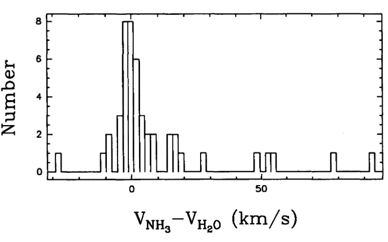
2.7 Distribution of the difference between the water maser peak veloc-ity and the velocveloc-ity of the associated ammonia emission Churchwell

et al. (1990) 36

2.8 Illustration showing the proposed evolutionary scenario of a cluster

of high-mass stars (Purcell, 2006) 39

2.9 Maser evolutionary sequence proposed by Ellingsen et al. (2007). 40 2.10 Comparison between the derived bolometric luminosity and the

mass of the cores from Rathborne et al. (2010) 46

3.1 Integrated "CO emission observed by Bains et al. (2006) with the two regions surveyed for water masers overlaid. 50 3.2 Locations of the OH, methanol and water masers overlaid on an

image of the integrated "CO 55

3.3 Three colour GLIMPSE image of the G 333 GMC overlaid with

the locations of the masers. 56 3.4 Spectra of the 22 GHz water maser sources discovered in this survey. 58 3.5 ATCA spectra of the 22 GHz water maser sources detected in the

search that have been previously discovered. 59

LIST OF FIGURES

3.6 The mean velocity profile of the 13 C0 emission averaged over the entire field of observations from Bains et al. (2006) overlaid with the velocities of the detected water masers 72 3.7 Box plots of each of the 13 C0 clump properties split into the

cate-gories of yes and no, referring to water maser presence and absence

respectively 79 3.8 Box plots of the 1.2 mm dust clump properties split into the

cate-gories of yes and no, referring to water maser presence and absence

respectively 83 3.9 Box plots of the "CO (left) and 1.2 mm dust (right) clump

prop-erties split into the categories of yes and no, referring to methanol maser presence and absence respectively 85

4.1 Spectra of all the 12.2 GHz methanol masers detected in the search

towards 6.7 GHz methanol masers. 104

4.1 continued 105

4.1 - continued 106

4.1 - continued 107

4.1 continued 108

4.1 - continued 109

4.1 continued 110

4.1 continued 111

4.1 - continued 112

4.2 Log of 6.7 GHz peak luminosity versus the H2 number density of

the associated dust clump in cm -3 120

4.3 Log of 12.2 GHz integrated luminosity versus the H2 number den-

sity of the associated dust clump in cm -3 123 4.4 Log of the 6.7 GHz methanol maser peak flux density divided by

the 12.2 GHz methanol maser peak flux density versus the log of

the 6.7 GHz peak luminosity 129 4.5 Log of the 6.7 GHz methanol maser peak flux density divided by

4.6 Evolutionary sequence for masers associated with massive star for-

mation regions. 137

4.7 Colour-colour plot of GLIMPSE point source data. 139 4.8 Box plots of the 1.2 mm dust clump properties split in the

cate-gories of yes and no, referring to the presence or absence of 6.7 GHz

methanol maser emission respectively 144 4.9 Box plots of the 1.2 mm dust clump properties split in the

cate-gories of yes and no, referring to the presence of 6.7 GHz methanol maser emission with high and low luminosities respectively 145 4.10 Box plots of the 1.2 mm dust clump properties split in the

cate-gories of yes and no, referring to the presence or absence of 12.2 GHz methanol maser emission. 147 4.11 Box plots of the 6.7 GHz methanol maser properties split in the

categories of yes and no, referring to the presence or absence of 12.2 GHz methanol maser emission. 148 4.12 Box plots of the 1.2 mm dust clump properties split in the

cat-egories of yes and no, referring to the presence or absence of

de-tectable radio continuum emission. 150

5.1 Spectra of the 22-GHz water masers detected towards 1.2 mm dust

clumps. 178

5.1

—continuued

179

5.1 —co ntinuued 180

5.1

—continuued

181

5.1 —continuued 182

5.1

—continuued

183

5.1

—continuued

184

5.2 Water maser sources with no associated 1.2 mm dust clump emis- sion, detected within the target fields. 189 5.3 Latitude versus longitude diagram of the targeted 1.2 mm dust

clumps, showing the locations of the detected water masers. . . . 194 5.4 Histogram of the angular separation between the reported 1.2 mm

dust clump peak and the position of the water maser sources. . . 196

5.5 Separation from dust clump peak versus water maser flux density

plot. 197

5.6 Box plots of the 1.2-mm dust clump properties split in the cate- gories of y and , referring to the presence of water maser emission. 200

6.1 Spectra of the 22 GHz water masers detected towards sites of OH

and methanol masers. 231

6.1 —continuued 232

6.1 —continuued 233

6.1 —continuued 234

6.1 —continuued 235

6.1 —continuued 236

6.1 —continuued 237

6.1 —continuued 238

6.1 —continuued 239

6.1 —continuued 240

6.1 —continuued 241

6.1 —continuued 242

6.1 —continuued 243

6.1 —continuued 244

6.1 —continuued 245

6.1 —continuued 246

6.1 —continuued 247

6.1 —continuued 248

6.2 2004 peak water maser velocity versus 2003 peak water maser ve-

locity. 280

6.3 OH maser peak velocity versus methanol maser peak velocity. . . 287 6.4 Water maser peak velocity versus OH maser peak velocity. . . . . 291 6.5 Water maser peak velocity versus methanol maser peak velocity. . 292 6.6 Histogram of the number of solitary water masers detected in single

ATCA fields. 293

6.7 Colour-colour plot of GLIMPSE point source data showing sources

LIST OF FIGURES

7.1 Spectra of the 12.2 GHz methanol masers detected towards 6.7 GHz

MMB sources 329

7.1

-continuued

330

7.1

-continuued

331

7.1

-continuued

332

7.1

-continuued

333

7.1

-continuued

334

7.1

-continuued

335

7.1

-continuued

336

7.1

-continuued

337

7.1 -continuued 338

7.1

-continuued

339

7.1

-continuued

340

7.2 Histograms of the number of 6.7 GHz methanol masers versus Galactic longitude (top) and latitude (bottom) 357 7.3 Distribution of methanol masers in the southern portion of the

Galactic plane (top) and distribution of peak 6.7 GHz methanol maser velocity versus Galactic longitude (bottom) 358 7.4 Histogram of the number of 6.7 GHz sources in 5° Galactic

longi-tude ranges (top) and plot of the 12.2 GHz detection rates in each of these longitude ranges (bottom) 360 7.5 Longitude versus velocity 'crayon' plot showing all 6.7 GHz MMB

masers detected south of declination -20° 361

7.6 This figure is a 'zoomed in' version of Fig 7.5, showing a restricted velocity and longitude range which allows this highly populated region to be more clearly seen 362 7.7 Percentage of the 6.7 GHz methanol maser velocity range that the

6.7 GHz peak lies (top), and the 12.2 GHz lies (bottom) 367 7.8 Comparison between the 12.2 GHz emission (solid lines) and 6.7 GHz

emission (dashed lines) for sources showing stronger emission at 12.2 GHz for at least one spectral feature. 368

7.9 Comparison between the 12.2 GHz emission (solid line) and 6.7 GHz emission (dashed line) for 0326.641+0.611. 370 7.10 Comparison between the 12.2 GHz emission detected in 2008 June

(solid line) and 2008 December (dashed line) for eight of the most variable detected sources. 375 7.11 Histogram of the log 6.7 GHz methanol maser integrated

lumi-nosity using the near (purple) and far (black outline) distances calculated using Reid et al. (2009) (top) and Brand & Blitz (1993)

(bottom) 390 7.12 Histogram comparing the 6.7 GHz methanol maser integrated

lu-minosities using near (top) and far (bottom) distances calculated using Brand & Blitz (1993) (pink) and Reid et al. (2009) (black

outline) 391 7.13 Log of the 6.7 GHz integrated luminosity versus the log of the H2

number density of the associated 1.2 mm dust clump in cm'. The line of best fit is also plotted. 394 7.14 Log of the 6.7 GHz peak flux density divided by the 12.2 GHz

peak flux density versus the log of the 6.7 GHz methanol maser

integrated luminosity. 395 7.15 Log of the 6.7 GHz integrated flux density divided by the 12.2 GHz

integrated flux density versus the log of the 6.7 GHz methanol

maser integrated luminosity 396 7.16 Log of the 6.7 GHz peak flux density divided by the 12.2 GHz

peak flux density versus the log of the 12.2 GHz methanol maser

integrated luminosity 398 7.17 Log 12.2 GHz integrated luminosity versus the log of the 6.7 GHz

integrated luminosities. 400 7.18 Log 12.2 GHz integrated luminosity versus the log of the 6.7 GHz

integrated luminosities. 402 7.19 Log of the 6.7:12.2 GHz individual feature ratio versus the log

6.7 GHz peak luminosity for every spectral feature associated with

five methanol maser sources 403

LIST OF FIGURES

7.20 Log of the 6.7 GHz integrated luminosity versus the 6.7 GHz

methanol maser velocity range.

408

7.21 As for Fig. 7.20 with the addition of 6.7 GHz sources with OH but

no 12.2 GHz counterparts.

410

7.22 Log of the 12.2 GHz integrated luminosity versus the 12.2 GHz

methanol maser velocity range.

411

7.23 GLIMPSE colour-colour and colour-magnitude diagrams 415

7.24 GLIMPSE colour-colour and colour-magnitude diagrams, showing

sources with OH maser sounterparts.

416

8.1 Log integrated maser (water, 6.7 and 12.2 GHz methanol) flux

densities (Jy km s

-1

) versus log of the

H2

number densities (cm

-3

)

of the associated 1.2 mm dust clump. 423

8.2 Proposed evolutionary scheme for the common maser species in

high mass star formation regions.

429

2.1 Physical parameters of Hii regions (Kurtz, 2005) 17

3.1 22 GHz water masers detected within the survey regions. 57 3.2 Summary of associations with infrared, dust and molecular sources. 67 3.3 22 GHz continuum sources detected in ATCA observations. . . 68 3.4 Water masers with GLIMPSE point source associations. 71 3.5 Possible infrared and water maser source associations. 71 3.6 Separation from FIR sources, detected at 150 and 210 ,um. . . . 72 3.7 Water maser sources with nearby 13C0 clumps identified by Bains

et al. (2006) 74

3.8 Properties of the "CO clumps (Bains et al., 2006) 75 3.9 Water masers sources with nearby CS emission peaks. 75 3.10 Maser sources with nearby 1.2 mm dust clumps identified by Mook-

erjea et al. (2004) 77

3.11 Analysis of deviance table for the single term models computed

using the "CO clump properties as predictors 78 3.12 Summary table for the Binomial regression model for the "CO

analysis 80

3.13 Analysis of deviance table for the single term models (using the 1.2 mm dust clump properties), showing the AIC and the deviance together with the associated likelihood ratio statistic and p-value for the test of the hypothesis that the stated single model provides no better fit than the null model consisting only of an intercept. . 82 3.14 Summary table for the Binomial regression model, showing for

each predictor the estimated coefficient and the standardised z-value and p-z-value for the test of the hypothesis that A=0. . . . 82

4.1 Targeted 6.7 GHz methanol masers, detected 12.2 GHz methanol masers and associated 1.2 mm dust clump that they are associated

with 96

4.1 —

continued

97

4.1 —

continued

98

LIST OF TABLES

4.1 - continued 99

4.1 - continued 100

4.2 Absorption features that we detect at 12.2 GHz towards 6.7 GHz

methanol masers 102

4.3 Analysis of deviance table for the single term models; 1.2 mm dust clumps with and without 6.7 GHz methanol 142 4.4 Summary table for the Binomial regression model of 1.2 mm dust

clumps with and without 6.7 GHz methanol masers 143 4.5 Analysis of deviance table for the single term models, dust clumps

with and without highly luminous 6.7 GHz methanol masers. . . . 143 4.6 Summary table for the Binomial regression model of 1.2 mm dust

clumps with luminous 6.7 GHz methanol masers and those with

less luminous 6.7 GHz methanol masers 146

4.7 Analysis of deviance table for the single term models, dust clumps with 6.7 GHz methanol masers with and without 12.2 GHz methanol. 146 4.8 Summary table for the Binomial regression model of 1.2 mm dust

clumps with associated 6.7 GHz methanol masers with and without a 12.2 GHz methanol maser counterpart 149 4.9 Analysis of deviance table for the single term models, dust clumps

with 6.7 GHz methanol masers with and without 12.2 GHz methanol. 149

4.10 Analysis of deviance table for the single term models, dust clumps with and without associated 8 GHz radio continuum 151

5.1 ATCA observations: epochs and array configurations 156

5.2 H75 configuration antenna spacings 159

5.3 6D configuration antenna spacings 160

5.4 H214 configuration antenna spacings 161

5.5 6B configuration antenna spacings 162

5.6 Size of the synthesised beam in each of the array configurations 163 5.7 1.2 mm dust clumps (Hill et al., 2005) excluded from the target

list and/or subsequent analysis. 165

LIST OF TABLES

5.8 Target 1.2 mm dust clumps, probability of water maser association, followed by a description of the water maser observations including

any detections. 167

5.8

continued

168

5.8 —

continued

169

5.8

continued

170

5.8 —

continued

171

5.8 —

continued

172

5.8 —

continued

173

5.8

continued

174

5.8 —

continued

175

5.8 —

continued

176

5.9 Four water maser sources detected in the target fields that are not coincident with any detected 1.2 mm dust clump emission. . . 190 5.10 Analysis of deviance table for the single term models (using the

1.2 mm dust clump properties from Hill et al. (2005)) 199 5.11 Summary table for the Binomial regression model 199 5.12 Summary table for the Binomial regression model using only dust

clump radius 202

5.13 Summary of the categories of dust clumps where we find water

masers. 204

5.14 Average values of all of the 1.2 mm dust clump properties of sources that are associated with water masers, broken up into the

associ-ation categories 206 5.15 The average and median flux densities, and velocity ranges of all

of the detected water masers, broken into the different association

categories 208 5.16 Relationship between 6.7 and 12.2 GHz methanol and water maser

luminosities and associated H2 number densities of the 1.2 mm dust

clumps 209

6.1 Characteristics of the 379 22 GHz water masers detected towards

sites of OH and methanol masers 218

6.1 continued 219

6.1 — continued 220

6.1 — continued 221

6.1 continued 222

6.1 — continued 223

6.1 — continued 224

6.2 OH masers with no associated water maser emission 230 6.3 Water maser sources with associated OH and methanol masers as

well as 22 GHz continuum emission 249

6.3 continued 250

6.3 — continued 251

6.3 — continued 252

6.3 — continued 253

6.3 continued 254

6.3 — continued 255

6.3 continued 256

6.3 — continued 257

6.3 — continued 258

6.4 22 GHz continuum sources detected towards water maser sources. 260 6.5 The average and median water maser flux densities for the water

maser sources we detect. 284

6.6 Comparison between water maser associations and the presence of

associated 22 GHz radio continuum. 294

6.7 Comparison between water maser associations in our full sample with water maser associations for sources associated with EGOs. . 300

7.1 Characteristics of the 6.7 GHz methanol maser targets as well as the 12.2 GHz methanol maser emission that we detect. 312

7.1 — continued 313

7.1 — continued 314

7.1 — continued 315

7.1 — continued 316

7.1 —

continued

318

7.1 —

continued

319

7.1 —

continued

320

7.1 —

continued

321

7.1 —

continued

322

7.1 —

continued

323

7.1 —

continued

324

7.1 —

continued

325

7.1 —

continued

326

7.1 —

continued

327

7.3 Calculated methanol maser distances

379

7.3

continued

380

7.3

continued

381

7.3

continued

382

7.3

continued

383

7.3

continued

384

7.3

continued

385

7.3

continued

386

7.3

continued

387

7.3

continued

388

7.3

continued

389

7.5 Summary of results from linear regression analysis for data pre-

sented in Figs 7.14, 7.15 and 7.16

397

7.6 Summary of results from linear regression analysis for data pre-

sented in Fig. 7.18.

401

7.7 Average and median velocity ranges and luminosities of 6.7 and

12.2 GHz methanol masers broken into categories on the basis of

The process through which high-mass stars (M > 8M®) form is one of the

hottest topics in modern astrophyics, with implications for fields as diverse as galactic evolution and the epoch of reionization. We are yet to realise a unified theory of star formation or the mechanism through which high-mass stars are able to form. One of the difficulties is the lack of sequential signposts in identifying different evolutionary stages of star formation, especially during the early stages while the young stellar objects are still embedded in their natal molecular clouds.

A common phenomenon observed in active high-mass star forming regions is the presence of interstellar masers, particularly emission from the OH, water and methanol molecules. They are relatively common and intense making them one of the best, if not

the

best signposts of young high-mass star formation regions.

Observing interstellar masers allows us to probe stars at very early stages of formation and because these masers arise at radio frequencies, they are relatively unaffected by the dense, optical-obscuring gas and dust present at these earliest stages. Masers have long been regarded as powerful probes of the kinematics of star formation regions, but we are only recently beginning to be able to use masers to investigate aspects such as the physical conditions through comparison of observational data and maser pumping theories. Different maser species trace different physical conditions and have been hypothesised to signpost different evolutionary phases of high-mass star formation (e.g. Ellingsen et al. 2007).

I have investigated the presence or absence of water, OH and methanol masers associated with a large number of sources suspected of undergoing high-mass star

formation. Many observations were carried out to complete this project, utiliz-ing data from the Australia Telescope National Facility's Australia Telescope Compact Array (ATCA) and Parkes 64 m radio telescope and the University of Tasmania 26 m Mount Pleasant radio telescope. Specifically, the 22 GHz tran-sition of water, 22 GHz radio continuum and 12.2 GHz methanol masers have been searched for and we have uncovered a large number of new sources. Data collected through this series of observations has then been combined with pub-lished data (e.g. 6.7 GHz methanol masers,

OH

maser sources, 1.2 mm dust clumps, molecular data and mid-infrared sources) for these sources, in order to compare the characteristics of sources associated with different combinations of maser species. Throughout this work an emphasis has been placed on investigat-ing the relative evolutionary phases that the different maser species are tracinvestigat-ing and into gaining insight into the physical conditions that are associated with the presence or absence of the common maser species in high-mass star formation regions.

An introduction to the radio telescopes, data reduction and visualisation pack-ages, the statistical analysis used throughout this work, as well as a brief summary of each of the chapters, are presented in the sections that follow.

1.1 The radio telescopes

1.1.1 The University of Tasmania 26 m Mount Pleasant

radio telescope

it was tracking. The traditional telescope Azimuth-Elevation mount does not allow the tracking of objects overhead, but in general are more desirable as they are more compact, keeping the telescope lower to the ground and allowing better pointing accuracy.

The telescope is a prime focus instrument and has multiple receivers mounted on a movable platform, allowing the observations of frequencies between 600 MHz and 22 GHz. Both the 12 GHz and 22 GHz receivers where used in order to com-plete this work and are part of the multi-frequency receiver which is cryogenically cooled with liquid Helium to a temperature of around -250°C. This dramatically enhances the receiver's sensitivity as it decreases the thermal noise.

While few observations using the Mount Pleasant telescope are presented in this work, many hours of preparatory observations for the majority of the projects were completed. These observations allowed the feasibility of observation strate-gies to be completed, but also allowed us to gain an idea of the number of detec-tions and the kinds of results to expect from our proposed projects. Furthermore, they allowed us to use allocated time on the Australia Telescope National Facility instruments to be used in the most efficient manner, allowing us to observe large sample sizes which ultimately have lead an increase in science results.

1.1.2 The Australia Telescope National Facility

The Australia Telescope National Facility (ATNF) is a division of the CSIRO, which includes the ATNF headquarters located at Marsfield in Sydney, as well as the Parkes, Paul Wild and Mopra Observatories, located near Parkes, Narrabri and Coonabarabran, respectively (and are all located within NSW, Australia). The ATNF facilities operate under a semester based system with two application deadlines per year. Gaining time on these instruments is highly competitive since oversubscription rates are generally high, so time is prioritised according to rankings awarded by the Time Allocation Committee.

The Parkes 64 m radio telescope

The Parkes 64 m radio telescope is operated by the ATNF and is located about 380 km west of Sydney. The telescope is located at latitude latitude 32° 59' 54"

S, longitude 148° 15' 49" E. The surface of the dish is high precision aluminum millimeter wavepanels to a diameter of 17 m, perforated aluminum plate out to 45 m and then galvanized steel mesh out to 64 m. The telescope is a prime focus antenna with an azimuth-elevation mount. Parkes has receivers with allows observations between the frequencies of 0.44 and ,26 GHz.

Observations presented in Chapters 4 and 7 use the Ku-band receiver, oper-ating at ,--12 GHz. At this frequency the low efficiency of the outer panels of the telescope mean that it can be regarded as a —55 m telescope.

The Australia Telescope Compact Array

The Australia Telescope Compact Array (ATCA) is an array of six, 22 m anten-nas. Located about 500 km north-west of Sydney, the telescopes are situated at the Paul Wild Observatory and, like Parkes, are operated by the ATNF. The six antennas are located at a latitude of 30° and can be placed at stations along the 6 km track aligned east-west, as well as a 214 m northern spur. The location of the ATCA allows for full uv-coverage at high angular resolution for sources south of declinations of —24°. However, snap-shot observations of sources up to a declination of +48° are attainable, with perhaps the most problematic range of declinations being those close to a declination of zero degrees where the syn-thesized beam becomes highly elongated due to the East-West orientation of the array baselines.

The ATCA operates between frequencies of 1.3 and 105 GHz. In Chapters 3, 5 and 6, ATCA observations of spectral line and continuum data at 22 GHz, are presented.

1.2 Data reduction software

A number of data reduction and visualization packages have been used throughout Chapters 3 - 7. One of the most frequently used packages MIRIAD (Sault, Teuben & Wright, 1995) which is a radio interferometry data reduction package, widely used for the reduction of both continuum and spectral line data collected chiefly with the ATCA. MIRIAD can be used for all stages of data reduction, from loading

the data files, through to imaging fields, and extracting the required information from the images.

The images produced from the interferometric observations using MIRIAD were

inspected using kvis which is part of the Karma package of visualisation tools. Kvis is a tool which not only displays images and movies, but also allows multiple data sets to be loaded and displayed such that contours of one image can be overlaid on another, line profiles of multiple images can be overlaid. Images can also be annotated and exported from this package.

For single dish data, ASAP (ATNF Spectral line analysis package) has been

used for data reduction. This package was produced by the ATNF to reduce data from their single dish antennas, but has been adapted to reduce data from other antennas, such as the Mount Pleasant 26 m radio telescope. ASAP is based

on the AIPS++ package and the user interface uses an object oriented ipython

interactive shell. Due to this, scripting the data reduction process in python is relatively simple, allowing data reduction to be carried out very efficiently.

ASAP is very flexible and allows for non-standard data reduction to be carried

out with relative ease which was important in reducing the data presented in Chapters 4 and 7.

1.3 Statistical analysis

A number of the discoveries presented in this thesis are a result of the statistical analysis of the characteristics associated with the large data sets. Throughout, the statistical analysis package R' (R Development Core Team, 2006) has been used for this purpose. As well as standard statistical tests such as t-tests, chi-sqared tests and linear regression, slightly less widely applied analysis such as fitting Binomial generalized linear models (GLM) have been used. Since there are a number of cases where we have observations of masers towards either 1.2 mm dust clump data (Mookerjea et al., 2004; Hill et al., 2005) or molecular data (e.g. Bains et al., 2006), the fitting of GLMs to the data allows the characteristics of the sources associated with the masers to be compared with sources devoid of the maser species. Furthermore, GLMs do not require the tested variables to be independent and they allow for the prediction of future outcomes from the

analysis of the predictors.

GLMs have been used to investigate the properties of the molecular gas and dust in the regions with associated maser emission. They have been fitted to the maser presence/absence data using associated source properties (such as 13C0 and 1.2 mm dust clump properties reported by Bains et al. (2006) and Mookerjea et al. (2004); Hill et al. (2005) respectively), as predictors. A Binomial GLM predicts the probability, p,, of finding a maser in the

i

th

clump, in terms of the clump properties x1, x2, x3, . . . x. The model takes the form

y, Bin(1,p,)

Pt

log 130 + xi, + /32x2, + . . . + 13mx.

1 — Pt

where y, is the maser presence or absence in the

i

th

clump and /30, 01, 132 are the regression coefficients to be estimated.

To test the significance of individual clump properties all possible single term models can be fitted, and compared by analysis of deviance to the null model consisting of only an intercept. Stepwise model selection based on the Akaike Information Criteria (AIC) (Burnham & Anderson, 2002) was used to select the most parsimonious model with the greatest predictive power. The AIC is a trade off between goodness of fit and model complexity and is defined as

AIC = —2(max log likelihood) -I- 2(number of parameters)

with the preferred model being the model with the lowest AIC (Venables & Ripley, 2002).

For ease of comparison between the data sets box plots were commonly cre-ated for each of the clump properties. The solid horizontal line in each of these plots represents the median of the data. The box represents the 25th to the 75th percentile, while the vertical line from the top of the box represents data from the 75th percentile to the maximum value and the vertical line from the bottom of the box represents data from the 25th percentile to the minimum value. Ex-treme values are classified as outliers, and represented by dots, if their range from the 25th or 75th percentile (in the case of the minimum and maximum values of

clump properties, respectively) is greater than 1.5 times that of the interquartile range.

1.3.1 An example of GLM analysis

Here we step through an example of were a GLM has been fitted to a data set in Chapter 3, Section 3.4.4. In this case, particular portions of a giant molecular cloud have been searched for both water masers and 1.2 mm dust clump emission. A comparison between the locations of the water masers with the 1.2 mm dust clumps shows, not surprisingly, that each of the water masers is coincident with a 1.2 mm dust clump. In order to determine if there is any differences between the properties of the 1.2 mm dust clumps with associated water maser emission, compared to those without, we have fitted a binomial GLM to the water maser presence/absence data, using the 1.2 mm dust clump properties (e.g. radius, mass etc.) as predictors.

Firstly, we fit all possible single term models to see if any of the clump prop-erties alone can be used as an indicator of the likelihood of water maser presence. Basically, this is just a test of the hypothesis that the stated single term model provides no better fit than the null model which consists only of an intercept. In other words, this tests looks for a relationship between the y-values (e.g. values of 1.2 mm dust clump radius) and whether or not there is an associated water maser, i.e. to determine whether or not there is a slope between the two groups of data (the dust clumps with masers and those without). Table 3.13 gives the results of this analysis. The most important value in this table is the p-value. For example, for the dust clump property radius, the resultant p-value is 3.787e-07 which means that the null hypothesis can be rejected. From this we can as-sert that there is a statistically significant difference between the 1.2 mm dust clump measurements for sources with associated water masers compared to those without.

The second major piece of analysis is the stepwise model selection. Our model selection method tries to include as few of the dust clump properties as possible, while maintaining the ability to predict whether or not there is an associated water maser. This process is begun by adding in all of the predictors and then

deleting the one that causes the least reduction in the 'goodness of fit' (and so on), a process called backward elimination. Continuing the explanation of our former example (Chapter 3, Section 3.4.4), the results of this analysis are located in Table 3.14. In this table the only dust clump property presented is the dust clump radius. This does not indicate that the other dust clump properties are not related to the presence of the water masers, but rather, that the inclusion of these other properties failed to increase the predictive properties of the model. As stated in Section 3.4.4, the estimated regression relation is

pi

log

1— pi = —11.477+ 9.174xradius

where xradjus is the radius of the 1.2 mm dust clump in pc.

Since there is only one predictor included in this model, the physical implica-tions are easily determined, as discussed in Section 3.4.4. In the case where such a model has two or more terms, these implications become harder to decipher. In such cases, coefficients should not by considered individually, but instead as a whole. For instance, a hypothetical equation that includes a positive coeffi-cient for radius but a negative coefficoeffi-cient for mass, may give an indication that the masers are associated with the big clumps that perhaps have slightly lower densities than the other considered sources.

1.4 Thesis summary

Chapter 2 contains a review of the literature, and necessary background informa-tion.

In Chapter 3 I present a complete survey for water maser towards portions of the G 333 giant molecular cloud (covering a total area of almost half a square degree). Comparisons between the locations of the water and methanol masers with 13C0 and 1.2 mm dust clumps as well as infrared data are completed. From these data, a predictive model for water masers associated with 1.2 mm dust clumps was formed. This Chapter is essentially that presented in Breen et al.

(2007) with the addition of Section 6.4 from Bains et al. (2009).

Chapter 4 presents observations of 12.2 GHz methanol masers observed to-wards 6.7 GHz methanol masers associated with 1.2 mm dust clumps observed by Hill et al. (2005). The properties of these sources (such as the presence or absence of emission from the 12.2 GHz transition of methanol, as well as the properties of the associated 1.2 mm dust clumps) were compared with the locations of 8 GHz radio continuum emission (Walsh et al., 1998), OH masers (Caswell, 1998) and mid-infrared point sources and statistical analysis of these data have resulted in an evolutionary sequence for masers in high-mass star formation regions, placing quantitative estimates on the relative lifetimes for the first time. This work is that presented in Breen et al. (2010a).

Chapter 5 contains water maser observations carried out with the ATCA towards the majority of the 404 1.2 mm dust clumps presented in Hill et al. (2009). The 1.2 mm dust clumps with and without associated water masers are then compared to the predetermined probabilities of water maser presence using the model of Breen et al. (2007) (also see Chapter 3). Discussion of the current model for water maser presence associated with 1.2 mm dust clumps is given, and using the larger sample, refinements to this model are offered. In addition, comparison between the locations of the detected water masers with other maser species, radio continuum data and mid-infrared sources is carried out.

Chapter 6 presents water maser observations towards a statistically complete sample of ,--200 OH masers (Caswell, 1998) and a sample -400 methanol masers Caswell, Kramer & Reynolds (2009). Detection statistics as well as some analysis of water maser variability, peak velocity comparisons between the different maser species and associations with 22 GHz radio continuum and mid-infrared sources are presented. This work is that published in Breen et al. (2010b).

Chapter 7 contains 12.2 GHz observations towards all of the 6.7 GHz methanol masers detected in the Parkes Methanol Multibeam (MMB) south of declination —20°. This is the largest search for 12.2 GHz methanol maser ever completed, gaining a full sample of these masers in the southern hemisphere, south of — 20°. Detection statistics free from biases are derived for the first time along with numerous results uncovered from the comparison between the two methanol maser transitions, along with the characteristics of the sources that they are associated with.

Chapter 8 discusses all the individual projects together and here a conclusion is made using the combined results of Chapters 3 - 7. Along with the scien-tific implications of the numerous results given in Chapters 3 - 7, an updated evolutionary timeline for the common maser species in high-mass star formation regions is given.

masers and evolutionary tracers

In this chapter, a review of the literature relevant to the work contained in this thesis is presented. While an effort was made to include major works that have contributed to our knowledge of high-mass star formation, associated interstellar masers and different evolutionary tracers, due to the breadth of the topics cov-ered it has not been possible to include everything. Due to this, only necessary background information is given along with a number of examples of supporting publications from the literature.

2.1 The formation of high-mass stars

The characteristics of our Galaxy, as well as those throughout the Universe, have been dramatically influenced by high-mass stars. Throughout their short life-times, they infuse their immediate environments with immense amounts of energy through their powerful outflows, ultraviolet radiation, and finally, as energetic su-pernovae. Their eventual demise as supernovae also allows them to inject heavy elements into the interstellar medium. The important role that high-mass stars play throughout the universe is undeniable and yet little is known about the mech-anism through which they are able to form. Furthermore, through their study we hope to gain greater understanding of what is causing the low star formation efficiency in our Galaxy. And in particular, determine what is regulating the star

formation rate (e.g. supersonic turbulent flows (e.g. Mac Low & Kleesen, 2004) or magnetic fields that are supporting the molecular cloud against gravitational collapse (e.g. Shu, Adams & Lizano, 1987)).

The study of high-mass stars is hindered by the fact they they form in clus-ters, deeply embedded in high density gas and dust. This means that high-mass stars are highly obscured by their natal material, dramatically limiting their observation, since they they are inaccessible at optical, and often near-infrared wavelengths. Their formation in clusters also adds further complication since each member of the cluster can be at different evolutionary stages, as well as in a different mass range. Due to the conditions in which these influential ob-jects are born, the best tracers of their existence are limited to radio wavelengths (through observations of UCHii regions, masers), sub-mm dust continuum, far-infrared and mid-far-infrared wavelengths. Furthermore, these objects are rare (due to the steep dependence on mass in the initial mass function), evolve quickly and are located at relatively far distances. All of these facts have contributed to our lack of understanding of these sources.

While aspects of the way high-mass stars form is still under debate, the pro-cess that results in the formation of isolated low-mass stars is reasonably well understood, and the basic model of accretion (Shu, Adams & Lizano, 1987) is generally accepted. For stars greater than --,8 M®, the Kelvin-Helmholtz time

(the time it takes for the core to begin converting gravitational potential energy into heat) will be less that the free-fall time (the time scale of collapse). This implies that fusion begins before the object has stopped collapsing. The radiation pressure in these objects is great enough to stop spherical accretion, but since we know that stars with greater masses exist, there has to be a mechanism which allows them to acquire it.

Some (e.g. Bally & Zinnecker, 2005) have suggested that higher-mass stars form via mergers, or coalescence, of lower-mass stars. This theory is supported by the fact that high-mass stars are seen to form in clusters, whereas isolated low-mass stars are known. The problem with this scenario is that high-mass star formation would be restricted to the centres of large stellar clusters with very high densities; densities that are rarely present in any known clusters (Bonne11, Bate & Zinnecker, 1998).

The most widely accepted model for high-mass star formation is based on a 'scaled-up' version of the low-mass model, but with a few alterations. In order for the stars to gain enough mass to be considered high-mass stars, they must undergo much higher accretion rates through a disk which allows the radiation pressure to be overcome (e.g. Tan & McKee, 2004; Krumholtz et al., 2009).

Although the basic mechanisms through which low- and high-mass stars form are expected to be similar, the formation of high-mass objects occurs over shorter timescales due to the increased density and energy. In this model, the star is created through the collapse of a core that is embedded within a clump that is in turn embedded in a molecular cloud. A schematic of the hierarchical structure of this process is presented in Fig. 2.1. As the embedded young star is forming, it accretes matter allowing it to gain mass, some of which is lost by through bipolar outflows or jets (which also allows angular momentum to momentum to be shed). There is growing evidence that (at least for some stars) the initial collapse of the core which will go on to form stars is 'triggered' by one of several mechanisms: these are discussed in Section 2.1.4.

Kurtz (2006) summarises the formation of high-mass stars through the accre-tion model as follows:

• Gravitational collapse of the material in a molecular cloud occurs on the free-fall time scale of 10 5 years.

• A core forms when enough matter has collapsed, evolving on the Kelvin-Helmholtz time scale of 10 4 years.

• The density of the core increases, the core becomes optically thick and the energy released in the gravitational collapse begins to heat the core.

• Nuclear reactions begin and produce ultraviolet radiation which ionises the surrounding material.

Molecular Cloud

n--10' cm T--10 K 0-10 pc

HII Region

Figure 2.1: Schematic diagram of the hierarchical structures within molecular clouds (taken from Kim Koo (2001)). This illustration shows that molecular clouds have clumps which have cores. High-mass stars form within the hot cores, creating an UCHH region which is initially small but can become very extended as the source evolves.

A brief discussion of the each of the 'phases' of high-mass star formation are presented in the following sub-sections. Further discussion is presented in Section 2.3 which includes information of the best traces of the formation during these stages.

2.1.1 Giant molecular clouds

Giant Molecular Clouds (GMCs) form the largest structures within our Galaxy. Their size and structure is varied, but often fall in the range 20 - 100 pc, with masses in the range 104 - 106 M® (e.g. Beuther

et

al., 2007). GMCs are formed when gas and dust accumulate under their own gravity, allowing them to become more than a thousand times denser than the interstellar gas that surrounds them. Their composition is mainly molecular hydrogen although they also contain varied amounts of some heavier elements and molecular gas.

[image:40.564.158.371.96.311.2]

-, 102 cm-3 and -40 K respectively. The velocity dispersions of GMCs are typi-cally only a few km s -1 which can largely be attributed to turbulence within the clouds. Measurements of magnetic fields in molecular clouds have shown that they typically have field strengths of the order of several tens of ,u,G (e.g. Bourke et al., 2001).

The structure of a GMC is typically highly non-uniform, composed of high density and lower density regions and much higher density cores (which are the locations where star formation originates). The high-density, star forming re-gions of GMCs can be easily identified by sub-mm dust continuum emission (e.g. Mookerjea et al., 2004) and high density molecular-line tracers (e.g. Lo et al., 2009). These cores are discussed further in the next section.

The stars that are forming in these 'stellar nurseries' eventually cause the dissipation of the surrounding gas and dust through heating, stellar winds and other disruptions that they impart into their immediate environments. The net result of their action may quench further star formation, or alternatively, trigger a new generation of star formation (see Section 2.1.4 for further discussion of this).

2.1.2 Cold and Hot cores

Preceding the hot core phase in the high-mass star formation sequence is, not surprisingly, the cold core phase. Garay et al. (2004) identified four such objects from 1.2 mm dust continuum emission. Their derived sizes, temperatures and masses (radius = 0.2 - 0.3 pc, temperature < 17 K, and mass = 4 x 10 2 - 2 x 103 Mo ), combined with their lack of mid- or far-infrared counterparts highlighted their potential to eventually collapse and form high-mass stars. Since then, other 1.2 mm dust continuum surveys have found many more cold core candidates (e.g. Hill et al., 2005). These objects are often found embedded in infrared dark clouds (IRDCs), (e.g. Rathborne et al., 2010); extinction features identified against the bright Galactic mid-infrared emission.

temperatures of > 100 K are experienced along with densities > 107 cm' and a multitude of molecular lines are observable, including transitions that require high levels of excitation.

Since hot cores are found to be internally heated (e.g. Cesaroni et al., 1998), based on temperature gradients peaking near the center of the cores, they are now accepted as a stage of high-mass star formation that precedes the onset of a detectable UCHii region. Supporting evidence for this comes from the associated masers that are present during this phase, some of which have been seen to be tracing disks and bipolar outflows (e.g. TorreIles et al., 1998) which is consistent with the characteristics expected during this phase. Molecular line surveys have also frequently shown line wings when targeting hot cores, indicative of both infall and outflows (e.g. Fuller, Williams

Sz

Sridharan, 2005; Purcell et al., 2006).

2.1.3

Hii regions

MI regions are created when the young high-mass star begins ionising its

sur-roundings by emitting ultraviolet photons, creating an expanding bubble around the object. These sources are classified by their size and emission measure as per the values listed in Table 2.1. For many years, UCHII regions were considered as one of the earliest detectable stages of high-mass star formation, but in recent years, advances in this field have allowed the identification of the other earlier phases already mentioned.

Wood & Churchwell (1989) found 75 UCHTI regions in the first large survey of these objects and noted that this number was inconsistent with the expected observable lifetime of these objects (of < 3 x 104 years). Wood

&

Churchwell (1989) further noted five different source morphologies (43 % unresolved, 20 % cometary, 16 % core-halo, 4 % shell, and 17 % irregular or multiply peaked).

Table 2.1: Physical parameters of MT regions (Kurtz, 2005).

Class of region Size Density Emis. Meas. Ionised mass (pc) (cm-3 ) (pc cm-6 ) Me

Hypercompact

<0.03

>10

6

>10

1

0

Ultracompact

<0.1

>10

4

>10

7

-

,

10

-2

Compact

<0.5

>5x10

3

>10

7

,

1

Classical

,

10

—100

-40

2

r-10

5

Giant

,

100

,

-30

-

,

5x10

5

10

3

-10

6

Supergiant

>100

-40

r-10

6

10

6

-10

8

object. Kurtz (2006) remark that from the typical sizes of UCHii and

hyper-compact Hii regions may indicate that hyperhyper-compact Hii regions just represent

the ionised gas around a single star where as an UCHN region corresponds to a

.

cluster of stars.

These hypercompact HI' regions are classified by their small sizes and large

emission measures (see Table 2.1). Kurtz (2005) comment that UCHii regions

typically show radio recombination line widths of 30 - 40 km s

-1

, while those

detected towards hypercompact Hii regions often show much broader line widths

(e.g. Sewilo et al., 2004). Since the first hypercompact HI' region was identified

by Gaume et al. (1995), the list of known examples of this class of sources has

grown (e.g. Murphy et al., 2010; Sewilo et al., 2008).

2.1.4 Triggered star-formation

Evidence for the evolution of one high-mass star causing the birth of a new

generation of high-mass stars is growing (so called 'triggered star formation').

Elmegreen (1998) summarized three three distinct mechanisms through which

triggered star formation could occur:

-61•351%Y

-6140a

-61.4sur

4

•

3 ,

13641.00' 006

tam

Figure 2.2: Images of RCW 79 showing a superimposed image of the 8 image from GLIMPSE (orange) and the Ha image from SuperCOSMOS (turquoise) on the

left, and 1.2 mm dust continuum emission on the right (Zavagno et al., 2006).

• gas accumulating into a dense shell or ridge that causes the gravitational collapse into cores ('collect and collapse');

• gravitational instabilities induced by clouds colliding ('cloud-cloud colli-sions').

In 'collect and collapse' an expanding H11 region sweeps up a dense shell of molecular material which can result in its fragmentation into clumps. Further disturbances can then trigger the collapse of the created clumps which results in star formation. Zavagno et al. (2006) shows one of a growing number of sources where there is evidence for 'collect and collapse' induced star formation around the Galactic Hii region RCW 79. Fig. 2.2 shows both a superimposed 8 pm GLIMPSE image and Ha image of the HI' region and a 1.2 mm dust continuum image. The comparison of these images shows that there is a layer of cold dust that traces the edge of the ionized region that has fragmented into clumps. In some of these clumps there is evidence for active high-mass star formation (as traced by masers and compact Hit regions).

formation, can also disrupt star formation by causing the dispersion of gas and dust.

2.2 Interstellar masers

Interstellar masers are key tools for investigating the formation of high-mass stars. The masers reside in the dusty molecular envelope or torus of a high-mass star in its early stage of formation, and are a sensitive probe for discovering stars in this embryonic state when the star is not visible because of obscuration from the dust. Many species and transitions of interstellar masers have been detected towards high-mass star formation regions, but the most common and strong transitions are from OH, methanol and water molecules. Analyses carried out in this thesis is limited to main-line OH, 6.7 and 12.2 GHz methanol (Class II transitions) and 22 GHz water masers. Due to this, the review of the literature is mostly limited to these transitions, along with some discussion of Class I methanol maser transitions.

Detailed studies of selected maser sites have been made comparing OH with water, and OH with methanol (Forster & Caswell, 1989, 1999; Caswell, 1997; Caswell, Vaile & Forster, 1995). These studies suggest that the maser spots of all species are usually contained inside a region of diameter less than 30 mpc (= 0.93 1015 m = 0.93 1017 cm 6200 au 0.1 light year), corresponding to an angular diameter of about 1 arcsec at a typical distance of 6 kpc. Positional precision of about 1 arcsec is therefore needed to establish whether masers of different species originate from the same site.

Within many star formation regions, on a larger scale of 100 mpc or more, the Forster & Caswell (1989) and Caswell (1997) studies revealed many instances where a number of maser sites are present in a small cluster, often with different combinations of maser species present. There has been considerable speculation that the various combinations are indicative of massive young stars at a different evolutionary stage, or in a different mass range (e.g. Ellingsen et al., 2007), since the different masers are known to trace different physical conditions (e.g. Cragg, Sobolev

&

Godfrey, 2002).

as tools to study star formation, however, the pace of advancement has recently accelerated. The proliferation of complementary high-resolution observations of star formation regions at millimetre through mid-infrared wavelengths means that this trend is likely to continue. Ideally, we would like to use masers to probe the physical conditions in the regions where they arise and the recent advancements in quality, unbiased survey data will aid enormously in this way.

In the following sections, particulars about the common maser species that are detected towards high-mass star formation regions are presented. Further, more specific information is presented at the introductions of Chapters 3 - 7.

2.2.1 OH

masers

The discovery of the first interstellar maser was from the OH line by Weaver et al. (1965), who announced the discovery of `mysterium ) . Since their discovery, they have commonly been thought to reside in the compressed zone just outside the expanding Hii region (e.g. Cook, 1968; Baart

&

Cohen, 1985) which is in

agreement with the model of Elitzur & de Jong (1978). Cragg, Sobolev & God-frey (2002) support the idea that OH masers are pumped by infrared radiation from warm dust (chiefly, although line-overlap is also required), just like Class II methanol masers, and suggest that it is the difference in the chemistry of the cores which decides whether emission from one or both species is seen.

Main-line OH maser emission at 1665 and 1667 MHz are by far the strongest and most populous of the OH maser lines, but other excited and satellite-line OH transitions exists in star formation regions, e.g. 1612, 1720, 6030, 6035, 13441 MHz. Caswell

&

Haynes (1987) found, in observations towards more than

100 southern OH sources, that the 1665 MHz transition is usually stronger than the 1667 MHz transition (typically by a factor of 3) and that it is detected towards 90 % of the 1665 MHz sources. Interferometric observations of Caswell (1998) confirmed that the two strong transitions were coincident to within an arcsec.