Completeness for the modal
µ-calculus:
separating the combinatorics from the dynamics
Sebastian Enqvist
Fatemeh Seifan∗ [email protected]
Yde Venema [email protected]
Institute for Logic, Language and Computation University of Amsterdam
PO Box 94242, 1090 GE Amsterdam,The Netherlands
August 2016
∗
Abstract
Themodal mu-calculus is a very expressive formalism extending basic modal logic with least and greatest fixpoint operators. In the seminal paper introducing the formalism in the shape known today, Dexter Kozen also proposed an elegant axiom system, and he proved a partial completeness result with respect to the Kripke-style semantics of the logic. The problem of proving Kozen’s axiom system complete for the full language remained open for about a decade, until it was finally resolved by Igor Walukiewicz. Walukiewicz’ proof is notoriously difficult however, and the result has remained somewhat isolated from the standard theory of completeness for modal (fixpoint) logics. Our aim in this paper is to develop a framework that will let us clarify and simplify parts of Walukiewicz’s proof. We hope that this will also help to facilitate future research into completeness of modal fixpoint logics, including fragments, variants and extensions of the modal mu-calculus.
Our main contribution is to take the automata-theoretic viewpoint, already implicit in Walukiewicz’s proof, much more seriously by bringing automata explicitly into the proof theory. Thus we further develop the theory of modal parity automata as a mathemat-ical framework for proving results about the modal mu-calculus. Once the connection between automata and derivations is in place, large parts of the completeness proof can be reformulated as purely automata-theoretic theorems. From a conceptual viewpoint, our automata-theoretic approach lets us distinguish two key aspects of the mu-calculus: theone-step dynamics encoded by the modal operators, and thecombinatorics involved in dealing with nested fixpoints. This “deconstruction” allows us to work with these two features in a largely independent manner.
More in detail, prominent roles in our proof are played by two classes of modal au-tomata: next to the disjunctive automata that are known from the work of Janin & Walukiewicz, we introduce here the class of semi-disjunctive automata that roughly cor-respond to the fragment of the mu-calculus for which Kozen proved completeness. We will establish a connection between the proof theory of Kozen’s system, and two kinds of games involving modal automata: asatisfiability gameinvolving a single modal automaton, and a consequence game relating two such automata. In the key observations on these games we bring the dynamics and combinatorics of parity automata together again, by proving some results that witness the nice behaviour of disjunctive and semi-disjunctive automata in these games. As our main result we prove that every formula of the modal mu-calculus provably implies the translation of a disjunctive automaton; from this the completeness of Kozen’s axiomatization is immediate.
Mathematics Subject Classification (MSC2010): 03B45; 03B70; 68Q60; 91A43.
1
Introduction
The modalµ-calculus The modalµ-calculusµMLis an extension of basic modal logic with least and greatest fixpoint operators. In the shape known today, it was introduced by Dexter Kozen [36], building on earlier work by others, including de Bakker & Scott [3], Park [49], and Pratt [54]. Since then it has been the subject of extensive research, see [1, 27, 8] for some surveys.
The µ-calculus has its roots in computer science, where it serves to unify and provide a foundation for the various modal logics that have featured as specification languages for programs and reactive systems. For example, linear temporal logicLTL[52, 23], computation tree logic CTL [13] and its extension CTL? [19] can all be embedded into the µ-calculus (see [15] for the non-trivial case ofCTL?), as can propositional dynamic logicPDL[53] and Parikh’s dynamic logic of games GL [48]. In this sense, the µ-calculus serves as a “universal” modal specification language.
Besides this important role in formal verification, it has become increasingly clear over the years that the modalµ-calculus also has a rich and beautiful meta-theory, and deserves a place in “pure” (mathematical) logic as well as in computer science. A paper that highlights this is the work by d’Agostino & Hollenberg [14], which shows that theµ-calculus enjoys several nice model-theoretic properties such as a Lyndon theorem and a Los-Tarski preservation theorem. Among the results obtained, the most striking is perhaps the interpolation theorem, which shows that the µ-calculus has the very stronguniform interpolation property. This property fails for first-order logic, but has previously been shown for a select number of logics, most famously intuitionistic logic [51], but also basic modal logic [24, 70].
The modal µ-calculus is a natural extension of basic modal logic, and retains many of its good properties. For example, Kozen [37] showed that the finite model property is pre-served and, improving on a series of earlier results, Emerson & Jutla [20] could pin down the complexity of the satisfiability problem for theµ-calculus as beingexptime-complete. While
basic modal logic has apspace-complete satisfiability problem, already minor extensions of it
areexptime-hard, including the logic obtained by adding the global modality [66]. Moreover,
theµ-calculus retains what is often viewed asthe defining property of modal logic, namely, its tight link with the notion ofbisimilarity. For modal logic, this is highlighted by van Benthem’s celebrated characterization theorem [4], exhibiting modal logic as the bisimulation-invariant fragment of first-order logic. It turns out that theµ-calculus is also the bisimulation-invariant fragment of an important system, namely monadic second-order logic (MSO). In the context of applications in process theory, this result, due to Janin & Walukiewicz [31], can be seen as an expressive completeness theorem, stating that all “relevant”MSO-formulas can be expressed in the modalµ-calculus.
axiom system adds a single axiom schema and a rule schema to handle the fixpoint operators. Together, the new axiom and rule schemas express in a straightforward way the equivalent characterization of the least fixpoint, well known from the Knaster-Tarski theorem, as the least pre-fixpoint. The axiom captures the pre-fixpoint property:
ϕ[µx.ϕ/x]→µx.ϕ.
The rule schema, which is sometimes referred to as Park’s induction rule, expresses in an equally simple way thatµx.ϕ is indeed the least pre-fixpoint:
ϕ[γ/x]→γ µx.ϕ→γ
The problem of proving the completeness of this axiom system turned out to be rather hard: Kozen presented a proof only for a fragment of the µ-calculus, which he called the
aconjunctive fragment, and the completeness problem for the full language remained open for
more than a decade until it was finally solved by Walukiewicz in [72] — in the sequel we shall refer to the extended journal publication [73].
Theorem 1 (Kozen-Walukiewicz) Kozen’s deductive system provides a sound and com-plete axiomatization for the set of valid formulas of the modal µ-calculus.
Walukiewicz’ proof is widely considered to be very hard to understand, and while the Kozen-Walukiewicz completeness theorem is often cited and generally recognized as a land-mark in the theory of the modal µ-calculus, it has remained something of an isolated point in the completeness theory of modal (fixpoint) logic. Modal logic has a well established the-oretical framework for completeness theory [6], with many standardized techniques such as canonical models and filtration, and sweeping general results like Sahlqvist’s theorem. The completeness theorem for the modal µ-calculus, on the other hand, does not seem to have given rise to any comparable follow-up literature (some exceptions to this rule will be discussed in a moment).
If we try to diagnose this situation, two obvious differences between theµ-calculus and the modal logics that are covered by the general completeness theory come to mind. First, the
Rather, what is special about the modal µ-calculus are the combinatorial issues that arise with simultaneous fixpoints, especially in the presence ofalternation between least and greatest fixpoints (i.e., mutual dependencies between least and greatest fixpoint operators). There is some evidence that this is indeed the crucial threshold: PDL, CTL, and flat fixpoint logics all sit inside the alternation free fragment. Also quite telling is that for the dual-free fragment of Parikh’s game logic, completeness is proved by a gentle modification of the proof for PDL [48], while for the full logic GL (which spans the whole alternation hierarchy, see [5]), finding a complete system of axioms remains an intrigueing open problem. In addition, the “exceptions” that we just mentioned, that is, the few papers that do address complete-ness questions for modal logics with explicit fixpoint operators and do make a link with the Kozen-Walukiewicz result, seem to support our claim. For instance, all papers that report positive results based on (relatively) easy proofs, seem to focus on settings where the alter-nation hierarchy collapses: ten Cate & Fontaine [2] prove a completeness result for the set of µML-validities on the class of finite trees (where nontrivial least and greates fixpoints co-incide), while Kaivola [34] proves completeness for thelinear time modal µ-calculus, that is, the modalµ-calculus interpreted on the structure of the natural numbers with the successor relation (where the alternation hierarchy collapses at the alternation-free level). Doumane & coauthors [17] obtain stronger positive results for this linear-time interpretation ofµML, but only for fragments of the language. Similarly, Santocanale’s analysis of Kozen’s axiomati-zation in [61] indicates that familiar algebraic methods can only prove completeness for the alternation-free fragment of the language.
It is also worth mentioning that the only known completeness proof for CTL?, due to Reynolds [57], is quite complex. The logicCTL? can be seen as a fragment of the µ-calculus, and as such it is not alternation-free. However, it is less clear how the case of CTL? fits into our description. Rather than a fragment of the µ-calculus, it might be more natural to think of CTL? as a sort of combination of LTL with S5 modal logic, and furthermore the difficulties that Reynolds deals with in his proof do not seem to be primarily concerned with the combinatorics of simultaneous fixpoints. Similarly, the completeness proof forECTL?, due to Kaivola [35], seems to be based on regarding this extension ofCTL? as a combination ofS5 with the linearµ-calculus, rather than as a fragment of µML.
Finally, in passing we note that in this paper we focus on finitary proof systems. If one is happy to work with infinitary proof systems (or finitary systems derived from these by an appeal to the small model property of the modal µ-calculus), then completeness for the full language of µML can be obtained in more direct ways than by the Kozen-Walukiewicz proof, see for instance the work of Kozen [37], Walukiewicz [71], or J¨ager, Kretz & Studer [29].
Logic and Automata A mathematical framework for the modalµ-calculus that is tailor suited precisely to deal with the combinatorics of fixpoint alternation is the theory of finite automata. This places the µ-calculus in a long tradition connecting logic and automata theory, going back to the seminal work of B¨uchi, Rabin and others. As two landmark results in this tradition we mention B¨uchi’s result showing that finite automata and monadic second-order logic have the same expressive power over infinite words [9], and Rabins’ decidability theorem [55] for the monadic second-order theorySnS.
type of automata are the parity automata, indepently introduced by Mostowski [45] and Emerson & Jutla [20]. And indeed, most of the deep results on the modal µ-calculus have used parity automata in one way or another; in particular, Walukiewicz’ completeness proof heavily uses automata-theoretic ideas and insights. Specifically, the proof proceeds from the observation that the satisfaction problem is easy for formulas of a certain normal form, called
disjunctive formulas, that correspond to the µ-automata (here called disjunctive automata)
introduced by Janin & Walukiewicz in [30]. The strategy of Walukiewicz’ proof is thus to prove that every formula ϕ of the µ-calculus can be rewritten as a semantically equivalent disjunctive formula ϕb, such that the implication ϕ → ϕb is provable in Kozen’s system. In
a sense, this can be seen as re-establishing the equivalence of µ-calculus formulas and µ -automata as aproof-theoretic result.
Our aim Our main goal in this paper is to streamline, clarify and, where possible, sim-plify the proof of the Kozen-Walukiewicz completeness theorem for the modalµ-calculus, by exhibiting and further developing the key mathematical concepts underlying the proof. In particular, we set up aframework for dealing with the completeness problem, in the hope that this will help to facilitate future research into completeness of modal fixpoint logics, including fragments, variants and extensions of the modal mu-calculus. In addition, our approach leads to a number of new automata-theoretic concepts and results that we believe to be of inde-pendent interest. In the remainder of this introduction we outline some of our main ideas, novel concepts and technical results.
Automata, coalgebra and proof theory The main conceptual difference with the ap-proach taken by both Kozen and Walukiewicz is that automata feature far more prominently in our proof. That is, one of the main novelties in our approach is that we make an explicit and mathematically precise connection between the proof theory for the µ-calculus and the theory of modal parity automata. Following this idea, we may rework large parts of Kozens’s and Walukiewicz’ arguments in an entirely automata-theoretic framework, where we may clearly distinguish what we take to be the two main parallel aspects of the completeness proof: the combinatorics involved in reasoning with fixpoints, and the dynamics encoded in the semantics of the modal operators. The combinatorics is dealt with by a purely combina-torial framework that we will call “trace theory”. The dynamics is understood by studying the so-called “one-step logic”, a concept originating from the theory of coalgebraic logic.
suppress the use of categorical methods, we have chosen to keep the coalgebraic perspective implicit, with three exceptions.
First of all, it will often be convenient for us to work with a coalgebraic presentation of a Kripke structure S, viz., as a function σS mapping each state s to a small window on the
Kripke structure, consisting of the pair, formed by the set of proposition letters thatssatisfies, together with the collection of its (immediate) successors. Such “one-step unfoldings” can then be examined by means of formulas of the one-step language that forms the domain of the transition map of our automata — this is what the game-theoretic semantics of our automata will be based on. Starting from this, we will investigate theone-step logicof Kripke structures, involving notions like one-step equivalence and one-step completeness. One-step logic, stemming from the work on coalgebraic logic by Cˆırstea, Pattinson, Schr¨oder and others [12, 50, 64, 65], is then the second important tool that we will take from coalgebra. And third, we will make extensive use of the coalgebraiccover modality ∇; this modality, which was introduced by Janin & Walukiewicz [30] as the natural modality of their µ-automata, (and which features also prominently in Walukiewicz’ completeness proof), was independently introduced in the context of coalgebraic logic by Moss [43].
Returning to the global picture of our proof, on the one hand its “deconstruction” allows us to deal with the combinatorial and the dynamic concepts in largely separate frameworks. On the other hand, the use of modal parity automata will allow us to combine these two features, to understand where and how the two perspectives interact, and how they connect to each other. In particular, we will see that the trace theory of an automaton is largely determined by the shape of the formulas of the one-step language.
Technically, the way we achieve this is to work with the wider class of modal automata (introduced under the name of “alternating automata” by Wilke [74]), rather than passing directly to theµ-automata used by Walukiewicz. One might say that we introduce automata into the picture at anearlier stage: as mentioned, the main goal in Walukiewicz’ proof strat-egy is to show that every formula of the µ-calculus proves some formula that corresponds to a syntactic representation of a disjunctive automaton. By working with arbitrary modal automata, we can prove an analogous result by much more elementary techniques: every for-mula is provably equivalent to a forfor-mula in a normal form, that is the syntactic representation of somemodal automaton. Formally we provide a modal automatonAϕ for each formula ϕ
and a formulatr(A) for each modal automaton A, and prove the following proposition (with
≡K denoting provable equivalence with respect to Kozen’s axiomatization):
Theorem 2 For every formula ϕ∈µML, we have ϕ≡K tr(Aϕ).
Games and special automata The main tools that we employ in our automata-theoretic approach towards Kozen’s deductive system are two kinds of games for modal automata: the satisfiability game and the consequence game, and two special kinds of modal automata: next to the disjunctive automata, the class of semi-disjunctive automata.
The satisfiability game S(A) related to a modal automatonA, was introduced in [22] in
the more general setting of the coalgebraicµ-calculus. It is an infinite two-player game, that can be seen as a streamlined, game-theoretic analog for automata to what tableaux are for formulas. In this game, thedynamics of the semantics appears in the moves of the player ∃
( ´Eloise) who has the role of “model builder”, and attempts to construct a satisfying model one layer at a time, while constrained by the one-step transition structure of the automaton.
The combinatorics of the trace theory enters the picture through the winning condition
for infinite matches. As we shall see, each infinite match naturally induces a trace graph, an intricate graph structure of which the finite and infinite paths correspond to A-traces: finite and infinite sequences of states of the automaton A. The winning condition of S(A) states that, for∃ to win the infinite match, all infinite traces, corresponding to full branches through this graph, need to satisfy the acceptance condition of A. Intuitively then, the smaller and simpler the trace graph, the easier it is for her to win. In particular, it will be to her advantage if we restrict the use of conjunctions in the one-step language, since these correspond to branching in the trace graph.
As we shall prove, the satisfiability game is adequate in the sense that ∃ has a winning strategy inS(A) iff the automatonAis satisfiable, that is, has a non-empty language. Hence our overall approach towards the completeness proof will be to prove that for anyconsistent automaton A, ∃ has a winning strategy in the satisfiability game associated with A. This makes that we will generally “take sides” with ∃ in the satisfiability game.
Before moving on to the other game featuring in our proof, we mention that the game
S(A) comes in two flavours: the standard and thethin satisfiability game Sthin(A). The two versions of the game have identical sets of positions for ∃ and her opponent∀ (Ab´elard), the only difference being that inSthin(A) we curtail the power of∀ by restricting his moves.
Theconsequence game C(A,A0), an original contribution of this paper, is an infinite two-player game that can be seen as a kind of implication game between the two automata A andA0. Its moves revolve around one of the players, prosaically named “player II”, trying to establish some structural connection between the two automata to support the claim thatA impliesA0. We write A|=G A0 in case he succeeds, in the sense of having a winning strategy in the gameC(A,A0). This relation |=G is a strong consequence relation between automata,
indicating a close structural relation between the automata; for instance, we shall see that A|=G A0 implies thatA0 is a semantic consequence of A, but not vice versa.
The consequence gameC(A,A0) is tightly connected to the satisfiability gamesS(A) and
S(A0); for instance, we will see that an infinite match Σ of the consequence game naturally induces infinite matches of the two respective satisfiability games, and that the winning condition on infinite matches of the consequence game is formulated accordingly.
still of a shape that guarantees the trace theory of an infinite match of the satisfiability game to be well behaved. In fact, by restricting the use of conjunctions in the one-step formulas of a semi-disjunctive automaton, we can guarantee that the collection of bad traces associated with a match of the satisfiability game is finite (modulo a natural equivalence relation of cofi-nal equality). Another important observation is that the standard and the thin satisfiability game for a semi-disjunctive automaton A are equivalent in the sense that ∃ has a winning strategy in the one game iff this applies to the other game as well.
Main results Concerning the concepts that we just discussed, we prove a number of results that we consider to be of independent interest. Here we outline three contributions that stand out as lemmas in the main proof.
The first result, which involves the Boolean operations of conjunction and negation that we shall define on modal automata, provides an essential link between the consequence game and the thin satisfiability game. We say that an automaton has a (thin) refutation if player
∀has a winning strategy in the (thin) satisfiability game for the automaton.
Theorem 3 Let A and D be respectively be a semi-disjunctive and an arbitrary modal
au-tomaton such that A|=G D. Then the automaton A∧ ¬D has a thin refutation.
This result can be seen both as an automata-theoretic counterpart and as a significant strengthening of a key result in Walukiewicz’ proof, viz., his Lemma 36.
Our second main auxiliary result, which also concerns the consequence game, can be seen as a strengthening of a classic result, viz., thesimulation theorem for modal (or alternating) automata. Simulation theorems are among the pillarstones of automata theory. They gener-ally show that an automaton of certain given type can be transformed into, or “simulated” by, an automaton that recognizes the same language, but in which the transition structure is of a conceptually simpler kind. Typically this either means that the transition structure is deterministic rather than non-deterministic or non-deterministic rather than alternating. The simplest result in this category is the standard powerset construction for (finite) word automata [56]; other examples include the simulation of non-deterministic B¨uchi automata for streams (infinite words) by deterministic Rabin automata due to Safra [59], or the simu-lation of alternating parity tree automata by non-deterministic ones due to Emerson & Jutla [20]. In our terminology, the simulation theorem says that any modal automatonA can be simulated by a disjunctive automaton sim(A). Our contribution is to show that this can be strengthened as follows.
Theorem 4 The mapsim(·)assigns to each modal automatonAa disjunctive modal automa-tonsim(A) such that
(1) A|=G sim(A) and sim(A)|=G A;
(2) B[sim(A)/p]|=GB[A/p], for any modal automatonB which is positive in p.
stronger result since we place no restrictions at all on the automaton B that appears as a parameter (apart from requiring that all occurrences of the proposition letterpare positive). Note that Theorem 3 and Theorem 4 can be formulated and proved completely indepen-dently of any deductive system for the modalµ-calculus.
The third result that we want to mention here crucially involves Kozen’s axiomatization. Recall that as the main goal of our completeness proof, we stated our intention to prove that∃
has a a winning strategy in the satisfiability game for any consistent automatonA. Theorem 5 below states a slightly weaker version of this, phrased in terms of thethin satisfiability game.
Theorem 5 ∃has a winning strategy in the thin satisfiability game for any consistent modal
automatonA.
We will informally refer to this observation as “Kozen’s Lemma”, since it is an automata-theoretic version of Kozen’s partial completeness result for the aconjunctive fragment of the modal µ-calculus [36]. As a consequence of the fact that for semi-disjunctive automata the standard and the thin satisfiability game are equivalent, our Theorem 5 also yields a partial completeness result, stating that any consistent (formula corresponding to a) semi-disjunctive automaton is satisfiable.
Proof of completeness Bringing all these ideas and results together, as the principal lemma in our proof we obtain the following version of Walukiewicz’ main technical result, with≤K denoting provable implication with respect to Kozen’s axiomatization.
Theorem 6 For every formula ϕ ∈ µML there is a semantically equivalent disjunctive
au-tomatonD such thatϕ≤K D.
We prove this theorem by a formula induction, and it should not come as a surprise that the key inductive cases are those concerning the fixpoint operators. In particular, the case whereϕis of the formϕ=µx.a requires all of the machinery developed earlier on.
Finally, from Theorem 6, the completeness theorem is almost immediate. If ϕ is an arbitrary consistent formulaϕ, then by Theorem 6 it is semantically equivalent to a consistent disjunctive automaton D. But for disjunctive automata it is easy to prove that consistency implies satisfiability, and so we are done.
Future work Our hope is that our “deconstruction” of the results and methods involved in the proof of the Kozen-Walukiewicz completeness theorem will lead to a better widespread understanding of a difficult result, but also that it will serve as a stepping stone for future research. In particular, we believe that an important direction for future work is to provide complete axiomatizations of several extensions, variations of and systems related to the modal
µ-calculus. An example that we already mentioned is Parikh’s game logic, more directly related examples are theµ-calculus with converse [68] and the closely related guarded fixpoint logic [28], hybrid µ-calculus [63], probabilistic variants as in e.g. [42], or even inflationary modal fixpoint logic [16]. We should mention here that a complete axiom system for the hybrid
involves a bound on model sizes for satisfiable formulas, rather than the Park induction rule used in Kozen’s system. We are currently studying the problem of proving completeness for coalgebraic generalizations of theµ-calculus, and a result that covers all weak pullback- and finite set preserving functors is forthcoming in [21]. We hope to be able in the near future to extend this result further, covering systems like the monotoneµ-calculus [41].
Two additional possible directions of research deserve to be mentioned. First, an interest-ing task would be to aim for generic completeness results forfragmentsof theµ-calculus. This would be a continuation of the work of Santocanale & Venema in [62] which provides generic completeness results for flat fixpoint logics, and the main question would be whether it is possible to push these results beyond the flat and even alternation-free fragments. (Again, this naturally ties in with the problem of proving completeness for game logic.) Second, we would like to study the problem of completeness foraxiomaticextensions of theµ-calculus (as opposed to theexpressive extensions mentioned earlier). This would be another step towards bridging the gap between the study of modal fixpoint logics and general research in modal logic, where the study of axiomatic extensions of the minimal normal or classical modal logic is usually at the centre of attention. Although such extensions of the µ-calculus are relatively rarely mentioned in the literature, some research does exist that suggests they are worthy of investigation, see for example [25] for a study of the least fixpoint extension of the logicS4 in a topological context.
Overview of paper In section 2 we fix some notation and terminology on infinite games, and on elementary mathematics. Section 3 introduces the syntax and semantics of the modal
µ-calculus, and we define Kozen’s deductive systemKµ. Section 4 sees the appearance of the main characters of our work, viz., the modal automata; we also discuss their one-step logic, and define the translation fromµML-formulas to modal automata which is based on automata-theoretic operations that correspond to syntactic operators ofµML. In section 5 we define the two satisfiability games and the consequence game. Section 6 is pivotal to our paper: here we introduce the disjunctive and semi-disjunctive automata, and we prove Theorem 3. Section 7 is devoted to the proof of our strong simulation result, Theorem 4. In section 8, which can be read independently of the sections 5 – 7, we provide the translation back from automata to formulas, and we prove Theorem 2. In section 9 we focus on the proof of Kozen’s Lemma, Theorem 5. We wrap things up in the final section 10, where we prove our main lemma, Theorem 6, and we show how to derive the Kozen-Walukiewicz result, Theorem 1, from this. Finally, while we have made an effort to provide all main results with detailed proofs, we have put some of the more tedious arguments and derivations to an appendix.
The structure of the paper is shown in the following dependency graph, where the arrows represent the order in which individual sections may be read:
7
1 //2 //3 //4 //
'
'
5 //6 //
@
@
9 //10
8
@
2
Preliminaries
We assume familiarity with the basic notions concerning infinite games [27]. Here we fix some notation and terminology, also regarding elementary mathematical concepts.
2.1 Basic mathematical concepts and notation
Definition 2.1 The power set of a setA is denoted asPA, and its size as |A|.
Since binary relations play an important role in our work, we will frequently use the following notation.
Definition 2.2 The collection of binary relations over a setAis denoted as A].
Given a relation R ⊆ A×A0, we let DomR and RanR denote its domain and range, respectively; for a subsetB0 ⊆A0, we define RanB0R:=RanR∩B0. Furthermore, we denote
the converse relation ofRasR−1:={(a0, a)∈A0×A|(a, a0)∈R}, and we set R[a] :={a0 ∈
A0 |Raa0}. Given a relationR⊆A×A and a subsetB ⊆A, we let ResBR:=R∩(B×B)
denote therestriction of R toB.
Definition 2.3 Given a relation R ⊆A×A0, we define the following relations between PA
andPA0:
− →
PR := {(B, B0)∈PA×PA0 | for all b∈B there is ab0∈B0 withRbb0} ←−
PR := {(B, B0)∈PA×PA0 | for all b0 ∈B0 there is ab∈B withRbb0}
PR := −→PR∩←−PR.
The relationPR is called theEgli-Milner lifting ofR.
Definition 2.4 We write f : A →◦ B to denote that f is a partial map from A to B, and we denote the graph of f as Grf := {(a, f a) | a ∈ Domf}; here Domf denotes the domain of f. The composition of two (partial) functions f : A →◦ B and g : B →◦ C is denoted as
g◦f :A→◦ C.
Definition 2.5 Given a setA, we letA∗ andAω denote, respectively, the set ofwords (finite sequences) and streams (infinite sequences) over A. We will write both ww0 and w·w0 to denote the concatenation of the wordswand w0, and similar for the concatenation of a word and a stream. The last symbol of a word wis denoted aslast(w).
Two A-streams σ and τ are eventually equal, denoted as σ =∞τ, if there is a k∈ω such
thatσ(j) =τ(j) for all j≥k.
2.2 Graph games
Definition 2.6 A board game is a tuple G= (G∃, G∀, E, W) where G∃ and G∀ are disjoint
sets, and, with G := G∃∪G∀ denoting the board of the game, the binary relation E ⊆ G2
winning condition of the game. In aparity game, the winning condition is determined by a parity map Ω : G → ω with finite range, in the sense that the set WΩ is given as the set
of G-streams ρ ∈ Gω such that the maximum value occurring infinitely often in the stream (Ωρi)i∈ω is even.
Elements ofG∃ and G∀ are called positions for the players∃ and ∀, respectively; given a
position p for player Π∈ {∃,∀}, the setE[p] denotes the set ofmoves that arelegitimate or admissible to Π at p. In case E[p] =∅ we say that player Πgets stuck atp.
An initialized board game is a pair consisting of a board gameGand a initial positionp,
usually denoted asG@p.
Definition 2.7 A match of a graph game G = (G∃, G∀, E, W) is nothing but a (finite or
infinite) path through the graph (G, E). Such a match ρ is called partial if it is finite and
E[lastρ] 6= ∅, and full otherwise. We let PMΠ denote the collection of partial matches ρ
ending in a positionlast(ρ) ∈GΠ, and define PMΠ@p as the set of partial matches in PMΠ
starting at positionp.
The winner of a full match ρ is determined as follows. If ρ is finite, then by definition
one of the two players got stuck at the positionlast(ρ), and so this player loosesρ, while the opponent wins. Ifρ is infinite, we declare its winner to be ∃ ifρ∈W, and ∀otherwise.
Definition 2.8 A strategy for a player Π ∈ {∃,∀} is a map χ : PMΠ → G. A strategy
is positional if it only depends on the last position of a partial match, i.e., if χ(ρ) = χ(ρ0) wheneverlast(ρ) =last(ρ0); such a strategy can and will be presented as a map χ:GΠ→G.
A match ρ = (pi)i<κ is guided by a Π-strategy χ if χ(p0p1. . . pn−1) = pn for all n < κ
such thatp0. . . pn−1∈PMΠ(that is, pn−1 ∈GΠ). A Π-strategyχislegitimate inG@p if the
moves that it prescribes toχ-guided partial matches in PMΠ@pare always admissible to Π,
andwinning forΠ inG@pif in addition allχ-guided full matches starting atpare won by Π. A positionpis awinning position for player Π∈ {∃,∀} if Π has a winning strategy in the game G@p; the set of these positions is denoted as WinΠ. The gameG= (G∃, G∀, E, W) is
determined if every position is winning for either∃ or∀.
When defining a strategyχfor one of the players in a board game, we can and in practice will confine ourselves to definingχ for partial matches that are themselves guided byχ.
The following fact, independently due to Emerson & Jutla [20] and Mostowski [44], will be quite useful to us.
Fact 2.9 (Positional Determinacy) Let G = (G∃, G∀, E, W) be a graph game. If W is
given by a parity condition, then G is determined, and both players have positional winning
3
The modal
µ
-calculus
Although we assume the reader is familiar with the syntax and semantics of the modal µ -calculus, here we provide a quick recapitulation of the main notions that play a role in this paper. More detail on the formalism can be found in [27, 69].
3.1 Syntax
Throughout this paper we fix an (unnamed) infinite set of propositional variables.
Definition 3.1 The languageµMLof the modalµ-calculus is given by the following grammar:
ϕ::=p| ¬ϕ|ϕ∨ϕ|3ϕ|µx.ϕ,
where p and x are propositional variables, and the formation of the formulaµx.ϕ is subject to the constraint that the variable x ispositive inϕ, i.e., all occurrences of xin ϕare in the scope of an even number of negations. Elements ofµMLwill be calledmodal fixpoint formulas,
µ-formulas, or simplyformulas.
The collection of subformulas of a formula is defined as usual, as are the sets of, respec-tively, its free and bound variables. We let µML(X) denote the set of µ-formulas of which all
free variables belong to the set X.
Remark 3.2 In order to focus completely on the hard and intricate parts of the completeness proof, we restrict attention tomonomodal logic here, that is, we consider the version of modal logic with one single primitive modality 3. The completeness proof for the polymodal µ -calculus, where one has a family {hdi | d ∈ D} of modal diamonds, can be obtained by a straightforward adaptation of the monomodal case, and follows from our more general result
in [21].
As a convention, the free variables of a formula ϕare denoted by the symbols p, q, r, . . ., and referred to as proposition letters, while we use the symbols x, y, z, . . . for the bound variables of a formula. Throughout the paper we will use standard abbreviations, including the symbols >, ⊥, ∧, →, 2, V
, and W
(where the latter two symbols are used to denote arbitrary but finite conjunctions and disjunctions, respectively).
Definition 3.3 Let ϕ and {ψz | z ∈ Z} be modal fixpoint formulas, where Z is a set of
variables that are of free in ϕ. Then we let
ϕ[ψz/z|z∈Z]
denote the formula obtained from ϕby simultaneously substituting each formulaψz for zin
ϕ(with the usual understanding that no free variable in any of theψz will get bound by doing
so). In caseZ is a singletonz, we will simply writeϕ[ψz/z], orϕ[ψ] ifzis clear from context.
If Z = Y1]Y2, it will occasionally be convenient to write ϕ[ψz/z | z ∈ Y1, ψz/z | z ∈ Y2]
Fact 3.4 Let {ψy | y ∈ Y} and {χz | z ∈ Z} be sets of formulas that are indexed by two
disjoint sets of variables Yand Z. Then for every formulaϕ we have
(1) ϕ[ψy/y|y∈Y][χz/z|z∈Z] =ϕ
ψy[χz/z|z∈Z]/y|y∈Y, χz/z|z∈Z
(2)ϕ[ψy/y|y∈Y][χz/z|z∈Z] =ϕ
ψy/y|y ∈Y, χz/z|z∈Z
, provided no z∈Z occurs freely in anyψy.
We will sometimes make the assumption (but always explicitly) that our formulas are in negation normal form.
Definition 3.5 A formula of the modal µ-calculus is innegation normal form if it belongs to the language given by the following grammar:
ϕ::=p| ¬p|ϕ∨ϕ|ϕ∧ϕ|3ϕ|2ϕ|µx.ϕ|νx.ϕ,
wherep and x are propositional variables, and the formation of the formulasµx.ϕ and νx.ϕ
is subject to the constraint that the variable x is positive in ϕ, i.e., no occurrence of x inϕ
is in the scope of a negation.
We use the symbol η to range overµ andν.
3.2 Structures
Definition 3.6 Given a set S, an A-marking on S is a map m :S → PA; an A-valuation on S is a map V :A → PS. Any valuation V :A → PS gives rise to its transpose marking
V†:S →PA defined by V†(s) :={a∈A|s∈V(a)}, and dually each marking gives rise to
a valuation in the same manner.
Since markings and valuations are interchangeable notions, we will often switch from one perspective to the other, based on what is more convenient in context.
Definition 3.7 AKripke structure over a setXof proposition letters is a tripleS= (S, R, V) such that S is a set of objects called points, R ⊆ S ×S is a binary relation called the accessibility relation, and V is anX-valuation on S.
Given a Kripke structure S = (S, R, V), a propositional variablex and a subset U of S, we define V[x7→U] as the X∪ {x}-valuation given by
V[x7→U](p) :=
V(p) ifp6=x U otherwise,
and we let S[x7→U] denote the structure (S, R, V[x7→U]).
Remark 3.8 Occasionally it will be convenient to take a coalgebraic perspective on Kripke structures. WithXdenoting a set of proposition letters, for a given set S we define
KXS:=PX×PS,
that is,KXS denotes the set of pairs (Y, U) withY⊆Xand U ⊆S. In practice we will usually
A Kripke structure S = (S, R, V) over the set X can then be represented as a map σS : S→KS given by
σS(s) := (V†(s), R[s]).
This mapσSwill be called the (coalgebraic) unfolding map ofS.
The operation K is in fact a functor on the category of sets with functions, and while we do not focus on this, in order to have compact notation it will be useful to borrow the following bit of category theory. Note that any mapf :S→S0 gives rise to a map Kf from
KS toKS0, defined by
Kf : (Y, U)7→(Y, f[U]).
The only fact about this map that we shall need is that it satisfies the composition law, stating that
K(g◦f) =Kg◦Kf.
for any pair of composeable maps g, f.
3.3 Semantics
Definition 3.9 By induction on the complexity of modal fixpoint formulas, we define a meaning function [[·]], which assigns to a formulaϕ∈µMLitsmeaning [[ϕ]]S⊆Sin any Kripke
structure S= (S, R, V). The clauses of this definition are standard:
[[p]]S := V(p)
[[¬ϕ]]S := S\[[ϕ]]S
[[ϕ∨ψ]]S := [[ϕ]]S∪[[ψ]]S
[[3ϕ]]S := {s∈S |R[s]∩[[ϕ]]S6=
∅}
[[µx.ϕ]]S := \{U ∈PS |[[ϕ]]S[x7→U]⊆U}.
If a points∈S belongs to the set [[ϕ]]S, we writeS, sϕ, and say that ϕistrue at sorholds
ats, or that ssatisfies ϕ.
Definition 3.10 A modal fixpoint formula ϕ is valid, notation: |= ϕ, if [[ϕ]]S = S for any
structure S = (S, R, V), and satisfiable if [[ϕ]]S 6= ∅ for some structure S. Two formulas ϕ
and ψ areequivalent, notation: ϕ≡ψ, if [[ϕ]]S= [[ψ]]S for any structureS.
3.4 The cover modality
As mentioned in the introduciton, thecover modality ∇, which was independently introduced in coalgebraic logic [43] and in automata theory [30], plays a prominent role in our proof, just as in Walukiewicz’. It is a slightly non-standard connective that takes a finite set Φ of formulas as its argument.
Definition 3.11 Given a finite set Φ, we let ∇Φ abbreviate the formula
∇Φ :=^3Φ∧2_Φ,
Remark 3.12 Observe that the semantics of the cover modality can be expressed in terms of the Egli-Milner lifting of the satisfaction relation:
S, s∇Φ iffR[s]PΦ.
In words,∇Φ holds atsiff every successor ofssatisfies some formula in Φ and every formula in Φ holds in some successor ofs. From this observation it is easy to derive that, conversely, the standard modal operators can be expressed in terms of the cover modality:
3ϕ ≡ ∇{ϕ,>}
2ϕ ≡ ∇{ϕ} ∨ ∇∅,
where we note that∇∅ holds at a pointsiffs is a ‘blind’ world, that is,R[s] =∅.
3.5 Axiomatics
As mentioned in the introduction, Kozen’s axiomatization for the modalµ-calculus is obtained by adding the (pre-)fixpoint axiom and rule to the basic modal logic K. For completeness’ sake we give the definition of Kozen’s system here, taking a standard3-based axiomatization forK[6, Remark 4.7].
Definition 3.13 The axioms of the basic modal logicK are the following: (C) a complete set of axioms for classical propositional logic;
(NA) axioms stating that 3is normal (¬3⊥) and additive (3(p∨q)↔3p∨3q), while itsderivation rules are
(MP) modus ponens: from ϕand ϕ→ψ, deriveψ;
(Mon) a monotonicity rule: fromϕ→ψ derive3ϕ→3ψ;
(US) uniform substitution: fromϕderiveϕ[σ], for any substitutionσ.
Kozen’s deductive system Kµ is obtained by this by adding the following axiom schema and
rule to those ofK:
(Aµ) all prefixpoint axioms of the formϕ[µx.ϕ/x]→µx.ϕ;
(Rµ) Park’s prefixpoint rule: fromϕ[γ/x]→γ deriveµx.ϕ→γ.
A derivation inKµis a finite list ofµML-formulas, such that each formula on the list is either an axiom ofKµor obtained from earlier formulas by applying one of the derivation rules of
Kµ.
Definition 3.14 A µ-formula ϕ is derivable or provable, notation: `K ϕ, if there is a Kµ -derivation leading up toϕ. Given two formulasϕ and ψ, we say that ϕprovably implies ψ, notation: ϕ ≤K ψ, if the formula ϕ → ψ is derivable. The formulas ϕ and ψ are provably
equivalent, notation: ϕ≡K ψ, if ϕ≤K ψand ψ≤K ϕ. A formula isconsistent if its negation
is not provable.
Fact 3.15 Let ϕbe a modal µ-formula, and let Φ,Ψ be sets of modal µ-formulas. Then
(1) ∇Φ∧ ∇Ψ≡K
_
{∇{ϕ∧ψ|ϕRψ} |R⊆Φ×Ψ and(Φ,Ψ)∈PR}; (2) ∇{ϕ0∨ϕ1 |ϕ∈Φ} ≡K
_
∇{ϕi|(ϕ, i)∈Z} | Z ⊆Φ× {0,1},DomZ = Φ ;
(3) µx.µy.ϕ≡K µy.µx.ϕ;
(4) ϕ≡K ϕ0 for some effectively obtainable formula ϕ0 in negation normal form;
(5) ϕ≤K ψ only if ηx.ϕ≤K ηx.ψ;
4
Modal automata and their one-step logic
As mentioned in the introduction, one of the main goals of the present paper is to further strengthen the role of automata theory in the completeness proof for the modal µ-calculus. While Walukiewicz’s proof works directly with what we will call disjunctive automata, we will work with the wider class ofmodal automata [74] that we will introduce in this section.
A further goal in this section is to define a translation transforming a formula of the
µ-calculus into an equivalent modal parity automata. Of course, there are already a few different methods available for this transformation. Janin & Walukiewicz [30] first construct a tableau for the formula, which is then transformed into an automaton in which the states are certain distinguished nodes of the tableau. This method already produces anon-deterministic automaton (what we will call a “disjunctive” automaton), and so is not suited for our purposes since we want to work with the wider class of alternating modal automata introduced by Wilke [74]. It seems that the standard approach to this (see for instance [27], following Wilke), is to transform aµML-formulaϕinto an automaton in one go, by taking the states of the automaton to be syntactic items related toϕ(such as its subformulas or bound variables), and then (possibly) perform some postprocessing in order to get the device into the right shape. Our preferred method here will be to define the translation by induction on the complexity of formulas, making use of certain effective closure conditions on the class of modal automata. In fact, most (but not all) of the operations on automata that we will use to take care of the inductive step of the translation, are the ones used by Wilke in order to prove the correctness of his translation.
Before turning to the introduction of the modal automata themselves, we first define and discuss the one-step logic that determines the shape of their transition function. As mentioned in the introduction, the notion of a “one-step logic” stems from the literature on coalgebra [12], where it is used to obtain a modular approach to defining and studying logics for specifying the behaviour of a wide variety of coalgebras, or state-based evolving systems. The idea behind this logic is that it provides the syntax and semantics to extract information about the one-step behaviour of such a system, that is, the properties of one single unfolding of a state in the system. One-step logic thus comes with the notion of one-step syntax (a language consisting of one-one-step formulas), one-one-step semantics, and (possibly) one-step derivation systems and one-step model theory. This perspective is very compatible with the theory of automata operating on infinite objects, and Fontaine, Leal & Venema [22] introduced a notion of coalgebra automata of which the transition function maps states of the automaton to one-step formulas.
4.1 One-step logic
Modal automata are based on themodal one-step language. This language consists of modal formulas of rank 1, built up from proposition letters (which must appear unguarded) and
variables (which must appear guarded). In practice, the variables of a one-step formula will
always be states of some automaton.
following grammar:
π ::=⊥ | > |p|π∧π|π∨π,
wherep∈P. Given two setsXand A, we define the set1ML(X, A) ofmodal one-step formulas over Awith respect to Xinductively by
α::=⊥ | > |p| ¬p|3π |2π|α∧α|α∨α,
with p∈Xand π∈Latt(A).
Observe that the set of modal one-step formulas overA with respect to Xcorresponds to the set of lattice terms over the set {p,¬p|p∈X} ∪ {3π,2π |π ∈Latt(P)}. Note too that elements from the two parameter sets, Xand A, are treated quite differently in the syntax of one-step formulas: all occurrences of elements of X, corresponding to the proposition letters, must be unguarded, whereas the elements ofA, corresponding to bound variables of a formula and to states of our modal automata, may only occur in the scope of exactly one modality.
Modal one-step formulas will serve to provide the type of the transition map of a modal automaton, which will map states of the automaton to modal one-step formulas over the set of states. Intuitively, in a succesful “run” of a modal automaton on a Kripke structure, given that some state s in a Kripke structure is visited by some state aof the automaton, the run should provide a “local valuation” of the states of the automaton over the set of successors of
s, in such a way that the formula assigned to the statea becomes true. So a run of a modal automaton proceeds step-by-step, at each moment considering a local window into the Kripke structure as seen from the particular statesthat is currently being visited. In order to make these intuitions precise, we need a semantics for modal one-step formulas. This is given by one-step models.
Definition 4.2 Fix setsX and A. Aone-step frame is a pair (Y, S) where S is any set, and Y⊆X. A one-step model is a triple (Y, S, m) such that (Y, S) is a one-step frame andmis an
A-marking onS.
Observe that with this definition, the coalgebraic representation of a Kripke structure (S, R, V) can now be seen as a function σS mapping any state s∈S to a one-step frame of which the carrier is a subset of S.
We now turn to the semantics based on one-step models:
Definition 4.3 Theone-step satisfaction relation 1 between one-step models and one-step formulas is defined as follows. Fix a one-step model (Y, S, m). First, we define the value [[π]] of a lattice formula π overA by induction, setting [[a]] ={s∈ S |a∈m(s)} for a∈A, and treating conjunctions and disjunctions in the obvious manner.
Now we define the one-step satisfaction relation by giving the usual clauses for conjunction and disjunction, and the following clauses for the literals and modal operators:
- (Y, S, m)1 ¬p iff p /∈Y.
Two one-step formulas α and α0 are (one-step) equivalent, notation: α ≡1 α0, if they are
satisfied by the same one-step models.
Examples of one-step equivalent pairs of formulas include the familiar axioms of modal logic, such as2(a∧b) ≡1 2a∧2b, but also formulas involving the nabla modality, such as
∇B∧ ∇B0 ≡1 _{∇{b∧b0 |bRb0} |R⊆B×B0 and (B, B0)∈PR} (cf. Fact 3.15(1)). One particular kind of one-step models will be of special interest to us.
Definition 4.4 Given a set A, we define the canonical A-marking on PA as the map IA :
B7→B (that is, the identity map onPA). More generally, for any subsetBofPA, we consider the markingIAB:B →PX.
For any one-step formula α ∈ 1ML(X, A) and any element Γ ∈ KPA, say Γ = (Y,B), we abbreviate (Γ, IAB)1α as Γ1I α, and we denote [[α]]1 :={Γ∈KPA|Γ1I α}.
The main result about the modal one-step language that we shall need later is the following one-step version of the usual bisimulation invariance result for modal logic, i.e. all one-step formulas are invariant for bisimulations between one-step models in a precise sense. Observe that the definition below makes use of the (Egli-Milner) relation lifting of Definition 2.3.
Definition 4.5 Let (Y, S, m) and (Y0, S0, m0) be one-step models with respect to A and X. We say that these models areone-step bisimilar if they satisfy the following conditions:
(atomic)Y=Y0;
(forth) for alls∈S, there iss0∈S0 with m(s) =m0(s0); (back) for all s0 ∈S0, there iss∈S withm(s) =m0(s0).
We write (Y, S, m) ↔1 (Y0, S0, m0) to say that (Y, S, m) and (Y0, S0, m0) are one-step bisimilar.
We can now state the one-step bisimulation invariance theorem:
Proposition 4.6 (One-step Bisimulation Invariance) Let (Y, S, m) and (Y0, S0, m0) be any two one-step models with respect A and X. If (Y, S, m) ↔1 (Y0, S0, m0), then both one-step models satisfy the same formulas in 1ML(X, A).
We consider a useful instance of the one-step bisimulation invariance theorem: pick any set W, let Γ = (Y, S) be any one-step frame in KW, and let f : W → W0. Then any A -marking m on f[S] gives rise to the marking m◦f on S, and clearly the one-step models (Γ, m◦f) and (Kf(Γ), m) are one-step bisimilar:
(Γ, m◦f)↔1(Kf(Γ), m).
We also remark on a variant of the one-step bisimulation invariance theorem that we will make use of later. It can be thought of as a combination of one-step bisimulation invariance and a monotonicity property of one-step formulas, which we obtain since all variables in A
appear positively in any one-step formula in1ML(X, A).
Definition 4.7 Let (Y, S, m) and (Y0, S0, m0) be one-step models with respect to A and X. We say that (Y0, S0, m0) one-step simulates (Y, S, m), notation: (Y, S, m) →1 (Y0, S0, m0), if
(atomic)Y=Y0;
(forth) for alls∈S, there iss0∈S0 with m(s)⊆m0(s0);
(back) for all s0 ∈S0, there iss∈S withm(s)⊆m0(s0).
Proposition 4.8 (Preservation) Let (Y, S, m) and (Y0, S0, m0) be any two one-step models with respect A and X. If (Y, S, m) →1 (Y0, S0, m0), then any formula in
1ML(X, A) that is satisfied by (Y, S, m) is also satisfied by (Y0, S0, m0).
Finally, we introduce the key property of the one-step logic for the purposes of our com-pleteness proof: the one-step logic already enjoys a sort of comcom-pleteness property with respect to the Kozen proof system, which we will lift to a completeness result for the full mu-calculus. This is the one-step completeness theorem, stated below.
Theorem 4.9 (One-step completeness) Letα∈1ML(X, A) be a one-step formula, and let
σ : A → µML(X) be a substitution such that the formula α[σ] is consistent. Then there is a one-step model (Y, S, m) such that (Y, S, m) 1 α and for all s ∈ S, the set of formulas
{σ(a)|a∈m(s)} is consistent.
Proof. We begin by rewriting the one-step formulaα as a disjunction of conjunctions of the shape:
γ∧ ♥1π1∧...∧ ♥nπn
whereγ is a conjunction of literals over X, each ♥-operator is a modality ♥i ∈ {3,2}, and
eachπi is a lattice formula over A. Using the equivalences in Remark 3.12, we can rewriteα
into a disjunction of formulas of the form
γ∧ ∇Π1∧...∧ ∇Πn,
where each Πi is a finite set of lattice formulas over A. Now apply Fact 3.15(1) repeatedly,
and then distribute the conjunct γ over disjunctions, to obtain a disjunction of formulas of the shapeγ∧ ∇Π where Π is a finite set of lattice formulas overA.
Focusing on a disjunct of the shape γ ∧ ∇Π, we may assume that each member of Π is in disjunctive normal form. Now we can apply Fact 3.15(2) repeatedly to each member of Π (and again, distribute the conjunct γ over disjunctions) to pull the disjunctions outside the scope of the modalities. In the end we obtain a formula β ≡K α in a certain normal form, viz.,β is a disjunction of formulas of the form
γ∧ ∇{^B1, ...,
^
where γ is a conjunction of literals over X and B1, ..., Bk are subsets of A. We thus find
thatα[σ]≡Kβ[σ], soβ[σ] is consistent, which by propositional logic means that at least one disjunct
γ∧ ∇{^σ[B1], ...,
^
σ[Bk]}
is consistent. We construct a one-step model Y, S, m by setting S = {B1, ..., Bk}, m is the
identity map onS, and Yis the set of proposition letters pinXthat appear as a conjunct in
γ. It is easy to see that
Y, S, m1γ∧ ∇{^B1, ...,
^
Bk}
and it follows thatY, S, m 1 α. It remains only to check that each conjunction V
σ[Bi] is
consistent - but were it not, the formula 3V
σ[Bi] would be inconsistent by the normality
axiom for the diamond, and we reach a contradiction since 3V
σ[Bi] is a conjunct of the
consistent formulaγ∧ ∇{V
σ[B1], ...,Vσ[Bk]}. qed
4.2 Modal automata
We now formally introduce modal automata.
Definition 4.10 Fix a set of proposition letters X. Amodal X-automaton A is a quadruple (A,Θ,Ω, aI) where A is a finite set ofstates, aI is thestart state, Ω :A → ω is the priority
map, while the transition map
Θ :A→1ML(X, A)
maps states to one-step formulas.
Some basic concepts concerning modal automata are introduced in the following defini-tions:
Definition 4.11 The (directed) graph ofAis the structure (G, EA), where aEAb ifaoccurs
in Θ(b), and we let A denote the transitive closure ofEA. IfaAb we say that ais active inb. We writea ./Ab ifaAband bAa.
A cluster of A is a cell of the equivalence relation generated by ./A (i.e., the smallest
equivalence relation onAcontaining./A); a clusterCisdegenerate if it is of the formC ={a}
witha6./Aa. The unique cluster to which a statea∈A belongs is denoted asCa.
Definition 4.12 Fix a modalX-automatonA= (A,Θ,Ω, aI). Thesize ofAis defined as the cardinality of its carrierA.
With b ∈ A, let Ahbi denote the variant of A that takes b as its starting state, i.e., Ahbi= (A,Θ,Ω, b).
We writea<Ab if Ω(a)<Ω(b), and avAbif Ω(a)≤Ω(b). When clear from context we sometimes write<and vinstead, dropping the explicit reference to A.
Given a state aof A, we write ηa =µif Ω(a) is odd, and ηa=ν if Ω(a) is even, and we
callaanηa-state. The sets ofµ- and ν-states are denoted withAµand Aν, respectively.
We say that A is positive in a proposition letter p ∈ X if each occurrence of p in each
Modal automata run on Kripke structures, and acceptance is defined in terms of a two-player game, the acceptance game. The two players have opposing goals: one player ∃ (or “Eloise”) wants to defend the claim thatAacceptsS, and the opposing Player∀(“Abelard”) wants to establish the opposite. The game connects the one-step logic to Kripke structures, and the main thing to notice is that for any Kripke structureS= (S, R, V) over X, any given states ∈ S gives rise to a one-step frame (V†(s), R[s]) consisting of the variables in X that are true ats, together with the set ofR-successors of s.
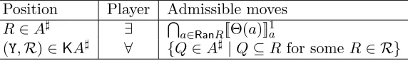
Definition 4.13 LetA= (A,Θ,Ω, aI) be any modal X-automaton, and let S= (S, R, V) be any Kripke structure. Theacceptance game A(A,S) forA with respect toS is defined as in the following table:
Position Player Admissible moves
(a, s)∈A×S ∃ {m:R[s]→PA|(V†(s), R[s], m)1 Θ(a)}
m ∀ {(b, t)|b∈m(t)}
Winning conditions are the usual ones for parity games. That is, the loser of a finite match is the player who got stuck. An infinite match (a1, s1)m1(a2, s2)m2(a3, s3)m3. . . induces a
streama1a2a3. . .over the alphabetA, and we declare the winner of this match to be∃if the
highest priority state that appears infinitely often in the worda1a2a3. . .has an even priority,
and∀ is the winner otherwise.
We say that A accepts the pointed structure (S, s) if (aI, s) is a winning position in the
acceptance game A(A,S), and write S, s A to denote that A accepts (S, s). We define [[A]]S :={s∈S |S, s A}, and we define L(A) (the “language recognized by A”) to be the
class of pointed Kripke structures accepted byA.
Definition 4.14 LetA= (A,Θ,Ω, aI) andA0= (A0,Θ0,Ω0, a0I) be two modal automata. We
say that A(semantically) implies A0, notation: A≤A0, if L(A)⊆L(A0), and that Aand A0 areequivalent, notation: A≡A0, if they recognize the same language, i.e., if L(A) = L(A0).
In the sequel we will need the following strong version of equivalence between automata.
Definition 4.15 Two modal automata A = (A,Θ,Ω, aI) and A0 = (A0,Θ0,Ω0, a0I) are
one-step equivalent, notation: A ≡1 A0, if A = A0, Ω = Ω0, aI = a0I, and Θ(a) ≡1 Θ(a) for all
a∈A.
It is obvious that one-step equivalence implies equivalence.
4.3 Operations on modal automata
Conjunction and disjunction
Suppose we are given modal automata A = (A,ΘA,ΩA, aI) and B = (B,ΘB,ΩB, bI). We
define the automaton A∧B= (C,ΘC,ΩC, aC) as follows:
- aC is some arbitrarily chosen object, andC is defined to beA]B] {aC}.
- ΘC(aC) := ΘA(aI)∧ΘB(bI) and ΩC(aC) :=k+ 1 where k is the maximum priority of
A,B.
- Fora∈A, ΘC(a) := ΘA(a) and ΩC(a) := ΩA(a).
- Forb∈B, ΘC(a) := ΘB(b) and ΩC(b) := ΩB(b).
Disjunction is handled in precisely the same manner, setting ΘC(aC) := ΘA(aI)∨ΘB(bI)
instead.
Negation
Negation corresponds tocomplementation on the side of automata, and for this we need the concept of theboolean dual α∂ of a one-step formula α:
Definition 4.16 First, we define the(boolean) dual of a lattice term over A, by setting:
a∂ :=a
(π∧π0)∂ :=π∂∨π0∂
(π∨π0)∂ :=π∂∧π0∂
With this definition in place, by putting
p∂ :=¬p (2π)∂ :=3π∂ (α∧β)∂ :=α∂∨β∂
(¬p)∂ :=p (3π)∂ :=2π∂ (α∨β)∂ :=α∂∧β∂
we inductively define the(boolean) dual of one-step formulas.
Observe that in this definition we see another clear example of the different role of the proposition letters and the automaton states in one-step formulas.
Given a modal automatonA= (A,Θ,Ω, aI) we define the automaton¬A:= (A,Θ0,Ω0, aI)
by setting, for eacha∈A: - Θ0(a) := Θ(a)∂ - Ω0(a) := Ω(a) + 1.
Modal operators
Given a modal automaton A = (A,Θ,Ω, aI), pick an arbitray object c, and define 3A = (A0,Θ0,Ω0a0I) by setting:
- A0 :=A] {c}, - a0I :=c,
- Θ0(a) := Θ(a) for a∈A, and Θ0(c) :=3aI,
Substitution
Let A = (A,Θ, aI,Ω) and B = (B,Λ,Ψ, bI) be modal automata, and assume that A is positive inx. We define the modal automaton A[B/x] as the structure (D,Θ0,Ω0, dI), where
D:=A]B, Θ0 is given by
Θ0(d) :=
Θ(d)[Λ(bI)/x] ifd∈A
Λ(d) ifd∈B.
The priority map Ω0 could have been defined as Ω]Ψ, but we find it convenient for later proofs to define Ω0 instead so that all states in A get higher priority than all states inB. So let n be the least even number greater than any priority inB. Then we set Ω0(b) = Ψ(b) for
b∈B, and Ω0(a) = Ω(a) +nfora∈A. (Clearly this will preserve the priority order among states inA and will not change the parities.) Finally, setdI =aI.
Fixpoint operators
We now turn to the definition of fixpoint operators on automata. For at least two reasons this is the most difficult case to handle. First, recall that in the one-step language associated with a modal automaton, the proposition letters (corresponding to the free variables of a formula) are treated rather differently from the states of the automaton (which correspond to the bound variables of a formula). We have good reasons to do so, but when constructing the automatonηx.Afrom an automatonAthere is a price to pay for this, related to the different status of the variablex in the two automata: while x is a free proposition letter in A, and so appears only in unguarded positions in the one-step formulas, it is treated as a state of
µx.Aand must therefore appear only guarded inµx.A. For this reason it will be necessary to
pre-process the automaton Aputting it in a shapeAx in which x is, in some sense, guarded.
Second, we have to be careful about how we go about this “pre-processing” of A. The reason for this will become clearer once we consider the satisfiability game for modal automata in Section 5. The game is played between Eloise, who wants to show that the automaton accepts some model, and Abelard, who wants to show that the automaton does not accept any model. It is important to realize that the roles of Eloise and Abelard are not treated symmetrically here, for the following reason: a match of the satisfiability game can be viewed as a collection of “virtual matches” of the acceptance game played at once. We shall see that the combinatorial difficulties involved in the completeness proof all stem from a common source: choices made by Abelard will generally cause the number of virtual matches we need to consider tomultiply, making the combinatorics of the game harder. For this reason, we want to take Eloise’s side as much as possible, and restrict the power of Abelard. In particular, since Abelard is in charge of conjunctions, we need to carefully control the shape of conjunctions that we introduce when we pre-process the automatonAintoAx.
Let us now turn to the construction of the auxiliary structure Ax, for which we shall require the following observation.
Proposition 4.17 For every modal X-automaton A positive in x∈X, and any state a∈A, there are formulas θ0a and θa1 in which x does not appear, such that
Proof. First rewrite Θ(a) as a disjunction
(x∧ψ0)∨...∨(x∧ψn)∨ψ00 ∨...∨ψm0
where each ψi and eachψ0j is a conjunction consisting of literals distinct fromx and formulas
of the form 2π,3π. This is then equivalent to
(x∧(ψ0∨...∨ψn))∨(ψ00∨...∨ψm0 )
and so we are done. qed
Convention 4.18 Relying on the previous observation, we fix from now on for every au-tomaton Aand a∈A, one-step formulasθa0, θa1 such that Θ(a)≡K (x∧θ0a)∨θ1a.
The construction of Ax is based on the following four ideas. First, since we do not formally allow proposition letters to appear guarded in the one-step formulas in the image of the transition map of an automaton, we introduce a new statex that we use to represent the variablex, in the sense that we put Θx(x) :=x. Second, we will “split” each stateainto two statesa0 anda1, taking care of theθa0- and theθa1-part of Θ(a), respectively. Thus we define
Ax := (A× {0,1})∪ {x}. Third, after this “change of base” of the automaton, we need to
ensure that the transition map Θx has the right co-domain (Ax). We can take care of this bysubstituting, in every one-step formula α∈1ML(X, A), each occurrence of a state aby the formula (x∧a0)∨a1. We shall denote the resulting substitution as κ : A → Ax. Fourth,
while we are mostly interested in the underlying automaton structure (AX,Θx,Ωx) ofAx, we do need to assign it an initial state. Our choice of (aI)1 is guided by the role of Ax in the proof of our main Lemma, Theorem 6.
Definition 4.19 Let A be any modal X-automaton which is positive in x ∈ X, and assume without loss of generality that the smallest priority in the image of Ω is greater than 0 (otherwise just start by raising all priorities in A by 2). Pick a new state x /∈A. Then we define theX-automatonAx= (Ax,Θx,Ωx, axI) as follows:
- Ax := (A× {0,1})∪ {x}. We write (a, i) as ai, fori∈ {0,1}.
- Θx(a0) :=θa0[κ] and Θx(a1) :=θa1[κ],
- Θx(x) :=x, - axI := (aI)1,
- Ωx(ai) := Ω(a) and Ωx(x) := 0.
Here,κ is defined to be the substitutiona7→(x∧a0)∨a1.
Note that the substitutionκinvolved in this construction does introduce new conjunctions, but in a very controlled manner: the only new conjunctions are of the formx∧a0 fora∈A,
i.e., we don’t introduce any conjunctions between states ai, for a ∈ A. This would not be
the case if we worked for example with the dual substitution κ∂ :a7→(x∨a0)∧a1. So the
Remark 4.20 The automaton Ax is not equivalent to A, in the sense that it does not ac-cept the same pointed Kripke structures asA does. On the other hand, it does contain all information that A does, and vice versa. The precise connection between A and Ax can best be expressed using thetranslation map that we will define in section 8. Running ahead of this, assume that we have defined, for each modal automaton A = (A,Θ,Ω, aI) a map
trA:A →µML assigning to each state a∈A an equivalent µ-calculus formula trA(a) in the sense thatAhai ≡trA(a) for each statea.
Phrased in terms of this translation map, the relation between Aand Ax is given by the equivalences
trA(a)≡(x∧trAx(a0))∨tr
Ax(a1)
and
trAx(ai)≡θia[tr
A(b)/b|b∈A]
which hold for alla∈A and i∈ {0,1}.
We now turn to the definition of the automata µx.A and νx.A; both constructs are variations of the auxiliary structure Ax. The key to understanding the definitions, and to proving correctness of the construction is the following proposition. We shall make use of it later on, when we consider the converse translation from automata to formulas. Since there we will be concerned withprovable equivalence, we formulate the next two propositions using the relation ≡K rather than the semantic equivalence relation ≡. Note that the semantic versions of the statements follow by the soundness of the axiom system.
Proposition 4.21 Let ϕ0, ϕ1 be any formulas in which the variable x appears positively.
Then:
µx.(x∧ϕ0)∨ϕ1 ≡Kµx.ϕ1
and
νx.(x∧ϕ0)∨ϕ1 ≡Kνx.ϕ0∨ϕ1
Proof. We consider the case forµfirst. One direction of the equivalence is immediate, since we haveϕ1 ≤K(x∧ϕ0)∨ϕ1. For the converse, we show thatµx.ϕ1 is a pre-fixpoint for the
formula (x∧ϕ0)∨ϕ1. To see this, we have:
((x∧ϕ0)∨ϕ1)[µx.ϕ1/x] ≡K ((µx.ϕ1)∧ϕ0[µx.ϕ1/x])∨ϕ1[µx.ϕ1/x]
≡K ((µx.ϕ1)∧ϕ0[µx.ϕ1/x])∨µx.ϕ1
≡K µx.ϕ1
For theν-case, again one direction is immediate since we have (x∧ϕ0)∨ϕ1≤K ϕ0∨ϕ1. For
the other direction we need to show thatνx.ϕ0∨ϕ1 is a post-fixpoint for (x∧ϕ0)∨ϕ1. We
reason as follows:
νx.ϕ0∨ϕ1 ≡K (νx.ϕ0∨ϕ1)∧(νx.ϕ0∨ϕ1)
≡K (νx.ϕ0∨ϕ1)∧(ϕ0[νx.ϕ0∨ϕ1/x]∨ϕ1[νx.ϕ0∨ϕ1/x])
≤K (νx.ϕ0∨ϕ1)∧ϕ0[νx.ϕ0∨ϕ1/x]
∨ϕ1[νx.ϕ0∨ϕ1/x]
= ((x∧ϕ0)∨ϕ1)[νx.ϕ0∨ϕ1/x]
![Table 3: The transition map and starting states of the automata A, Ax, µx.A and A[µx.A]](https://thumb-us.123doks.com/thumbv2/123dok_us/8383486.321215/42.612.103.504.116.243/table-transition-map-starting-states-automata-ax-ux.webp)

