MSc Thesis (Afstudeerscriptie)
written by
Haukur P´all J´onsson
(born July 28th, 1989 in Reykjav´ık, Iceland)
under the supervision of Frank van Harmelenand Jakub Szymanik, and submitted to the Board of Examiners in partial fulfillment of the requirements for the degree of
MSc in Logic
at theUniversiteit van Amsterdam.
Date of the public defense: Members of the Thesis Committee:
August 28, 2018 Ronald de Wolf Jaap Kamps
Abstract
In recent years interest has risen in combining knowledge representation and machine learning and in this thesis we explore Real Logic (RL). RL offers a novel approach to this combination. RL uses first-order logic (FOL) syntax and has a many-valued semantics in which terms are interpreted as real-valued vectors. By making assumptions about the model space and the relation between terms and predicates, we have a well-defined search procedure to search for models to our logical theory in a framework implementing RL called Logic Tensor Networks (LTN).
Acknowledgements
Contents
1 Theory 4
1.1 First Order Logic . . . 4
1.2 Many-valued Operators . . . 8
1.3 Real Logic . . . 11
1.4 Realization . . . 15
2 Experimental design 23 2.1 The Setting . . . 23
2.2 The Models . . . 26
2.3 Measures . . . 29
2.4 Hypotheses . . . 32
3 Experimental results 36 4 Discussion 43 4.1 T-norms and aggregations . . . 43
4.2 Biased features and variation . . . 45
4.3 Expressivity of LTN . . . 46
4.4 Logical constraints . . . 46
5 Conclusion 48
Introduction
Knowledge Representation and Reasoning is one of the core areas of artificial intelligence. The goal of knowledge representation is to model domain knowledge using a well-defined language along with inference rules to deduce facts. On the other hand, the goal of machine learning is to make predictions based on previous experiences by making assumptions about the underlying process. In both fields, the goal is to infer new knowledge given some input, but the structure of the input and assumptions made to do the inference differ quite a lot. One fundamental difference between the two approaches is the way objects are represented. Symbolic approaches tend to ignore the representation of the objects to be modelled and define symbolic inference to be invariant of representation. Machine learning approaches rely solely on the object’s representation when making predictions and one could say that a major factor in recent progress in machine learning is due to advances in learning better representations. Both approaches have enjoyed great success, but in order to solve tasks of increased complexity a combination of both approaches is in order. In particular for problems in which the problem statement is defined in terms of low-level representations and requires reasoning. Statistical Relational Learning (SRL) explores such tasks and tackles complex domains, which need to take into account uncertainty and complex relations between objects. In this thesis, we will use one such task, the task of Semantic Image Interpretation (SII) as an example to gain a better understanding of this combination. The goal of SII is to output a scene graph, given an image and some background knowledge about objects in the images. We want a solution to this task which is able to process an image from the raw pixel values and produces a graph in which the nodes have labels representing the type of object and labelled edges which describes their relationship in the image. Furthermore, we expect the predicted relations and labels to be consistent with some background knowledge. The labelling and edge-prediction tasks can be performed using machine learning alone, but a problem arises when the predictions are not consistent with the background knowledge. When the solutions are not logically consistent an object labelled as ”a cat” and another labelled as ”a tail” might be predicted to be in the ”part of” relation such that ”a cat is a part of a tail”, when it should much rather be ”a tail is a part of a cat” which we know from common sense knowledge. We would like to reject such predictions and better yet, improve the classifier in these cases.
This brings us to Real Logic (RL) (Serafini and Garcez, 2016; Serafini and d’Avila Garcez, 2016). RL is defined using the syntax of first-order logic (FOL) and has a many-valued se-mantics in which terms are interpreted in ann-dimensional space and consequently function symbols and predicate symbols as well. The intended application of RL is to describe knowl-edge about some domain using FOL and then represent the objects of that domain in a real-valued n-dimensional space. By assuming that terms which are represented ”close” to one another should have similar truth values, we can make predictions about otherwise
seen representations. By making this assumption, we can view the task of labelling and edge-prediction as knowledge base completion which is based on the representation of the terms. This further implies that all predictions are fundamentally limited by the represen-tation and functions considered. Thus, when evaluating RL we want to make sure that the representation is sufficiently informative, and together with the functions they are able to satisfy our theory. The particular functions considered are made concrete when we introduce the Logic Tensor Networks (LTN), which implement predicates of RL as a neural network. By working under the assumption that the functions considered are differentiable, we will use a search procedure from the gradient descent family.
In this thesis, we will evaluate RL by using the task of SII in two ways. First, we want to know how well RL is able to increase the logical consistency of predictions as well as over-all classification performance compared to a baseline model. This will give us an indication whether RL is able to combine learning based on low-level representation and logical reason-ing. Secondly, we want to know whether all instantiations of RL perform equally when using a search procedure from the gradient descent family. This will allow us to study the inner workings of RL and offer practical considerations based on theoretical and experimental evi-dence. Along the way, we formulate a number of hypotheses about the behaviour of RL and perform experiments to test them. This thesis is based on the works of Serafini et al. (2017) and Donadello et al. (2017) who show that RL using LTN is able to increase classification performance and performs well when trained on noisy data in the task of SII. In this thesis, we replicate these experiments and put forward other hypotheses. We confirm the original results but observe that the model does not learn in the way initially anticipated, the per-formance is somewhat unstable and some adjustments needed to be made to the structure of the model to achieve the same results. We start by making some observations how different implementations of RL will propagate the model’s error and quickly see that some implemen-tations will never work while other’s might. After viewing the experimental evidence and discussing the results we see conclusively that, out of the models we consider, a single class of models performs best. We experiment to see if the model is progressively able to satisfy the constraints and if more constraints make the predictions more logically consistent. We will see that the model does make the predictions more logically consistent and discuss how the model is able to make the predictions better. We hypothesize that adding more con-straints will decrease the variation in the performance of the model, and when we observe the opposite, we try to understand the origin of the variation. We do not explain the variation conclusively and only give a plausible explanation. Lastly, we compare the expressivity of the LTN to its predecessor. We quickly see when we compare the models that the LTN will probably outperform its predecessor in this setting and verify it during experimentation.
We start by setting the stage by defining all relevant concepts in section 1. In section 1.1 we define first-order logic, the notion of satisfiability and knowledge bases. In section 1.2 we define t-norms which generalise classical conjunction, its dual the s-norm, aggregation functions which serve as semantics for the universal quantifier. We also explore the partial derivatives of these operators and consider implementation issues. In section 1.3 we define the RL framework, its semantics and the maximum satisfiability problem. In section 1.4 we define the LTN and the Neural Tensor Network (NTN) as possible implementations for the predicates of RL and derive the gradient of a sentence’s generic grounding.
of SII and present different implementations of RL which will be considered. In section 2.3 we describe how we will evaluate the performance of the model as we are interested in the performances of the classification task, relation prediction as well as the logical consistency of predictions. In section 2.4 we state our experimental hypotheses and motivate them.
In section 3 we will go through the results of each experimental hypothesis and in section 4 we will contemplate the results of the experiments and try to explain them.
In section 5 we conclude the thesis and summarize the results.
Theory
In this section, we define all relevant concepts required for different parts of the thesis. In section 1.1, we start with some fundamental concepts in logic, namely the language and sat-isfiability. In section1.2, we move to many-valued extensions of conjunction and universal quantifiers. In section 1.3 RL is defined through the concept of a grounding, which is es-sentially an interpretation in which satisfiability is defined over the real field, in the range [0,1] and subsets of closed terms of the language are considered when evaluating the truth of universal quantification. In section 1.4 we make assumptions about the space of possible groundings, introduce the LTN, demonstrate how the gradient of the network is computed, make observations based on the structure of the gradient and compare with the operators defined in section 1.2.
1.1
First Order Logic
Let us start by introducing FOL syntax.
Definition 1(Vocabulary of FOLL). The vocabulary of First-order logic languageLconsists of variables x, y, z, . . ., logical constants ¬,∨,∧,⇒,∀,∃, non-logical constants which consist of individual constants a, b, c, . . ., predicatesP, R, . . . and function symbols f, . . . and other auxiliary symbols.
We letP be the set of all predicates,F be the set of all function symbols andC be the set of all constants for languageL. Each P ∈ P and eachf ∈ F is assigned a natural number, thearity of the functionα,α:P ∪ F →N. We writeα(P) =nto denote that the arity ofP
isn. We note that function symbols of arity 0 can be used instead of the individual constants but we refer to the constants C. We further assume that P and F are disjoint. The tuple
hF,P, σi is called thesignature ofL.
Definition 2 (Terms of L). The terms of FOLL are
• The individual variables.
• The individual constants.
• If f is a function symbol of aritynandt1, . . . , tn are terms, thenf(t1, . . . , tn) is a term.
• Nothing else is a term.
We refer to closed terms as terms which do not contain variables and denote them as
terms(L).
Definition 3 (Formulas of L). We define formulas for L inductively.
• If P ∈ P has aritynandt1, . . . , tnare terms then P(t1, . . . , tn) is a formula, also called
an atom or atomic formula.
• If ϕis a formula then ¬ϕ is a formula.
• If ϕand ψ are formulas then ϕ∨ψ and ϕ∧ψ are formulas.
• If ϕ is a formula which has at least one occurrence of variable x and does not contain
∀x or ∃x already, then ∀xϕ and ∃xϕ are formulas.
• Nothing else is a formula.
We letϕ⇒ψbe a short-hand for¬ϕ∨ψand useϕ(t1, . . . , tn) to denote a formula defined
over termst1, . . . , tn.
Definition 4 (Literal ofL). Let ϕbe an atom of L then ϕis a literal and ¬ϕis a literal.
Definition 5 (Clause ofL). Let ϕ1, . . . , ϕn be literals of L thenϕ1∨ · · · ∨ϕn is a clause of
L.
Using this definition we can create formulas of the form∀xP(y)∧R(x, y) which leads to the definition of bound and free variables and the corresponding closed and open formulas of
L.
Definition 6(Bound and free variables ofL). A variablex is bound iff it occurs inϕof the form∀xϕ. A variable x is free if it is not bound.
Definition 7 (Closed and open formulas of L). A formula in which no variables occur free is a closedformula, also called a sentence. Otherwise, the formula is open.
These definitions offer quite a range of writing FOL formulas and in later sections, we want to limit our discussion to sentences which have a particular structure, therefore we introduce three normal forms.
Definition 8 (Conjunctive Normal Form (CNF)). A formula of L is in CNF if it is a conjunction of clauses.
Definition 9(Prenex Normal Form (PNF)). A formula ofL is in PNF if all the quantifiers of the formula occur in a sequence at the beginning of the formula.
Definition 10(Skolem Normal Form (SNF)). A sentence of Lis in SNF if it is in PNF with only universal quantifiers.
Definition 11(Interpretation for FOL). An interpretation,I, for FOL is a pairhD,Vi, s.t.
D is a non-empty set of objects called the domainand V a valuation function which assigns objects fromD to individual constants and a set of ordered n-tuples of objects to predicates.
An interpretation is only defined in terms of the signature of theLand if we were to define truth of a sentence only based on the signature we would not be able to talk about the truth of a sentence which includes variables. This is addressed using theβ-variant of interpretation
I.
Definition 12 (β-variant of interpretation I). Let β be an individual constant and I and interpretation which assigns some element toβ, thenI* is a β-variant of interpretationI iff
I* and I differ only (if at all) in the assignment of β.
For formula ϕ, variable x, and constant c we denote ϕ[c/x] as the the formula in which all occurrences ofxhave been replaced byc. We now have everything in place to define truth in an interpretation of FOL.
Definition 13 (Truth in an interpretation). LetI be an interpretation for L, we define truth in interpretationI as
• If P is a predicate of arity n and c1, . . . , cn are individual constants thenP(c1, . . . , cn)
is true in I iffhV(c1), . . . ,V(cn)i ∈ V(P).
• ϕ is true in I iff ¬ϕis not true in I.
• ϕ∧ψ is true in I iffϕ and ψ are true inI.
• ϕ∨ψ is true in I iffϕ or ψ are true in I.
• ∃xϕis true in I iffϕ[c/x] is true in some β-variant of of I.
• ∀xϕis true in I iffϕ[c/x] is true in everyβ-variant of of I.
Definition 14 (Logical consequence). Let Γ be a set of sentences (possibly empty) and ϕ a sentence ofL thenϕis said to be a logical consequence of Γiff whenever Γ is true then ϕis true. We denote this with Γϕ.
When talking about particular interpretations, the following two notions are helpful.
Definition 15 (A model). Let Γ be a set of sentences of L and I be an interpretation s.t. for all ϕ∈Γ ϕis true in I thenI is a model of Γ, denoted as M.
This leads to the definition of satisfiability of a set of sentences.
Definition 16 (Satisfiability). Let Γ be a set of sentences of L. If there exists a model for Γ then Γ is satisfiable.
Now we come back to the normal forms.
Proposition 1 (Normal forms preserve satisfiability). A formula ϕ of L in some theory T
not in SNF or CNF can be converted to ϕ0 in CNF and SNF s.t. ϕ0 is in language L’ which has been extended with a new function symbol in the process of skolemization and if Mϕ
This proposition is a bit out of the scope of this thesis but let us briefly describe why we need to extend the language and therefore consider these extra caveats. In the process ofskolemization we replace existential quantifiers with new function symbols. Let us assume that we have a sentence ∀x∀y∃zϕ(x, y, z). When we read this sentence we read it such that for every x and given this x for all y there exists some z such that ϕ. The existence of z
is dependent on the interpretation of x and y. So when we want to replace the existential quantifier and substitute it with a new function symbol, the function must depend on x and
y.
Proof. We first transform ϕ to CNF. van Dalen (2004) (1.3.9) proves that such a trans-formation preserves satisfiability. We can then transform the CNF sentence to PNF. van Dalen (2004) (2.5.11) proves that such a transformation preserves satisfiability. Lastly, we can transform the PNF sentence to SNF through the process ofskolemization. In this process the language L is extended with a new function symbol for each existential quantifier in the formula, resulting in ϕ0. In van Dalen (2004) (3.4.4) it is proved if T `ϕthen the (Skolem) extension of T is conservative and for every model of T there is a Skolem expansion M0.
We could also have written ϕ0 ϕ, which is roughly the same. This proposition implies that instead of searching for models of ϕ we can equally search for models of ϕ0, which we will do.
But let us now transform a sentence to CNF, PNF and SNF.
Example 1 (A sentence converted to normal form).
∀x(P(x)⇒ ∃yR(x, y))
∀x(¬P(x)∨ ∃yR(x, y)) (CNF)
∀x∃y(¬P(x)∨R(x, y))(PNF)
∀x(¬P(x)∨R(x, f(x))) (SNF)
¬P(x)∨R(x, f(x))(short-hand)
Indeed, in the last step the∀ quantifier can be omitted since all variables are bound and thus implicitly universally quantified. We will therefore consider all variables bound for the rest of the thesis.
We have now defined all the required FOL concepts. In later sections, we will consider a knowledge base KB, which is a consistent set of sentences in SNF and CNF which describes knowledge in FOL and we look to extend it consistently. We will extend KB semantically rather than syntactically. That is, we start with some model which should satisfy our knowl-edge base and ask whether this model makesϕtrue, i.e. we check ifKB ϕIfϕis true, we add it to our set, if not, the negation is added toKB. One of the problems we will encounter is that finding a model for KB in the first place is hard, which should be no surprise. To allow a systematic search procedure through the model space, the model space is reduced by making assumptions about the domains and valuation functions considered.
1.2
Many-valued Operators
The truth of sentences in some natural language is not necessarily binary, in the sense that they are either true or false, but rather they might have varying degrees of truth. For example, assume that we have three people Bob, John and George. Bob is 180cm tall, George is 200cm tall and John is 160cm. We can attempt to model facts about these three people using FOL, one constant for each person and a single predicate for the property of being tall. Thus we might consider T all(George) to be true and T all(J ohn) to be false. But where would be place Bob? In this example we might consider putting Bob between John and George, thus using more values for truth than just two.
Fuzzy logic considers these generalizations to the truth values, in particular, truth values in the range [0,1] which we will use when RL is defined(Bergmann, 2008; Nov´ak, 1987). The continuity of the range is important, as later on it allows us to consider functions which are differentiable over this range. We will now define the generalizations for conjunction and disjunction which was developed along with many-valued logics but we will deviate from the conventional approach of fuzzy logic when it comes to universal quantification and rather use aggregation functions. The motivation here is that fuzzy logics are very strict when it comes to the truth value of universal quantification, considering the greatest lower bound over all
β-variants(Bergmann, 2008). So if one β-variant has a truth value of 0, the whole sentence has a truth value of 0. The RL framework is not this strict, and we will see that it is beneficial when computing the gradient but the cost is that the existential quantifier will have the same meaning as the universal quantifier. We are not too concerned with that, as we have already assumed that all sentences are in SNF which does not contain existential quantification.
We will now start with the generalization for conjunction and disjunction for truth values in the range of [0,1]. Triangular norms, or simply t-norms, are binary operations T on the interval [0,1] which satisfy the following conditions.
Definition 17 (T-norm). A triangular norm or t-norm is a binary operation. T : [0,1]×
[0,1]→[0,1]which satisfies the following conditions.
• T(x, y) =T(y, x) (commutativity)
• T(x, T(y, z)) =T(T(x, y), z) (associativity)
• y ≤z⇒T(x, y)≤T(x, z) (monotonicity)
• T(x,1) =x (neutral element 1)
T-norms serve to generalize the classical conjunction.
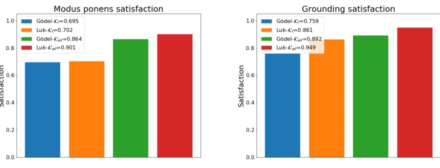
Example 2 (Examples of t-norms). See figure 1.1 for a contour plot of these functions.
• G¨odel t-norm: TG(x, y) = min(x, y)
• Lukasiewicz t-norm: T L(x, y) = max(x+y−1,0)
• Product t-norm: TP(x, y) =x·y
Due to associativity and commutativity T-norms can be extended to an n-ary opera-tion Klement et al. (2004), n∈N. We denote the extended t-norms with T(x1, . . . , xn).
Figure 1.1: The three t-norms; G¨odel, Lukasiewicz and Product t-norm and their values along [0,1]×[0,1]. Below the diagonal of the Lukasiewicz it takes the value 0.
• G¨odel t-norm: TG(x1, . . . , xn) = min(x1, . . . , xn)
• Lukasiewicz t-norm: T L(x1, . . . , xn) = max(Pin=1xi−(n−1),0)
• Product t-norm: TP(x1, . . . , xn) =
Qn i=1xi
The reader can verify that these norms are indeed generalizations of classical conjunction by checking that they result in the same values as the classical operators. At the same time, they all behave quite differently on the same inputs.
Example 4 (Examples of t-norm computations). Let x1 = 0.3, x2 = 0.5, x3 = 0.3, x4 = 0.1.
TG(x1, x2, x3, x4) = min(0.3,0.5,0.3,0.1) = 0.1
T L(x1, x2, x3, x4) = max(0.3 + 0.5 + 0.3 + 0.1−n+ 1,0) = 0
TP(x1, x2, x3, x4) = 0.3∗0.5∗0.3∗0.1 = 0.0045
We notice that the Lukasiewicz t-norm might often result in 0 when n is large. For example, with only two values, the average value needs to be greater than half to result in a positive number. We will make this observation concrete in section 1.4. We also observe that the product t-norm might cause issues in numerical computations, as computers do not handle multiplication of small numbers well. We will see that this is indeed an issue in hypothesis 1.1 but we will also present a solution to this in section 1.4 and follow up with hypothesis 7.
We now define the dual of a t-norm, a t-co-norm, also called s-norm1. Similarly, s-norms generalize the classical disjunction.
Definition 18 (S-norm). If T is a t-norm then S is an s-norm.
S(x, y) = 1−T(1−x,1−y)
Example 5 (Examples of s-norms). We give the duals of the previous examples
• G¨odel s-norm: SG(x, y) = max(x, y)
• Lukasiewicz s-norm: S L(x, y) = min(x+y,1)
1
• Product s-norm: SP(x, y) =x+y−xy
We also extend the s-norms to acceptn inputs and denote it asS(xn, . . . , x1).
Example 6 (N-ary s-norms). We extend the s-norms from our previous example.
• G¨odel s-norm: SG(x1, . . . , xn) = max(x1, . . . , xn)
• Lukasiewicz s-norm: S L(x1, . . . , xn) = min(Pni=1xi,1)
• Product s-norm: SP(x1, . . . , xn) = 1−Qni=1(1−xi)
Let us now explore how these s-norms work in computation.
Example 7 (Examples of t-norm computations). Let x1 = 0.3, x2 = 0.5, x3 = 0.3, x4 = 0.1.
SG(x1, x2, x3, x4) = max(0.3,0.5,0.3,0.1) = 0.5
S L(x1, x2, x3, x4) = min(0.3 + 0.5 + 0.3 + 0.1,1) = 0.9
SP(x1, x2, x3, x4) = 1−(0.7∗0.5∗0.7∗0.9) = 0.7795
Again, we see that the Lukasiewicz s-norm behaves quite strangely, we can almost trivially satisfy it just by adding enough xi > 0. We will make this observation more concrete in
section 1.4.
We have now introduced generalizations of conjunction and disjunction for truth values in the range [0,1] and now we will introduce aggregation functions, which are used for universal quantification in RL. The motivation to use the more generic aggregation functions instead of the standard fuzzy logic universal generalization is because they are simply too strict in the sense that a single β-variant can drag the truth value of the whole sentence down. We look for a softer approach than this. As an example, consider a sentence stating ”all swans are white”. We all know that this is sentence is false, as in fact ”most swans are white”. But stating it to be false seems to ignore a lot of the evidence that went into the statement. One could also consider the universal quantifier to be simply ”most” and thus the sentence would be true, but then the question arises, where to draw the line? What is ”most”? Instead, RL attempts to avoid this problem by considering generic aggregation functions2 so that one can choose based on a modelling scenario.
Definition 19(Aggregation function). An aggregation functionA is a functionA: [0,1]n→
[0,1] s.t.
• A(0) = 0.
• A(1) = 1.
If T = {x1, . . . , xn} then we denote A(T) to mean A(x1, . . . , xn) where we have ordered
the elements in some arbitrary order. One can think of aggregation functions which behave differently w.r.t. the order of inputs, and we consider those later on, but then we assume that the function itself orders the inputs.
2
Example 8 (Examples of aggregation functions). We give a few examples of aggregation functions which capture the intended definition.
• Arithmetic mean: Aari(x1, . . . , xn) =
Pn i=1xi
n
• Harmonic mean: Ahar(x1, . . . , xn) =
Pn i=1x
−1
i
n
−1
= Pnn i=1x
−1
i
• Minimum: Amin(x1, . . . , xn) = min(x1, . . . , xn)
• Maximum: Amax(x1, . . . , xn) = max(x1, . . . , xn)
Out of the example aggregation functions theAmin is the only candidate which is
consid-ered as in fuzzy logic (Bergmann, 2008).
We will also consider a different class of aggregation operators known as the Ordered Weighted Average (OWA). The OWA operator is an important aggregation function com-monly used in multi-criteria decision making, see Yager (1993).
Definition 20 (Ordered weighted average function (OWA)). An ordered weighted average functionA is an aggregate function s.t.
Aowa(x1, . . . , xn) = n
X
i=1
wixπ(i)
whereπ is a permutation from [n]to[n]s.t. xπ(i) is the i-th largest element ofx1, . . . , xn and
wi are the weights of the operator s.t. Pni=1wi = 1.
We use [n] to denote to the set {1,2, . . . , n}. Take note that for w1 = 1 and wi = 0 for
alli6= 1 then Aowa(x1, . . . , xn) =Amax(x1, . . . , xn). Similarly, forwn= 1 and wi = 0 for all
i6= n then Aowa(x1, . . . , xn) = Amin(x1, . . . , xn) and for wi = 1/n then Aowa(x1, . . . , xn) =
Aari(x1, . . . , xn).
We have now defined the many-valued operators we will consider for RL. The t-norms generalize the classical conjunction and s-norms generalize the classical disjunction. The treatment of many-valued universal quantification as aggregation functions is proposed as a more general approach than the standard fuzzy universal quantifiers, but we will show in the next section that this comes with a cost. Furthermore, in section 1.4, we will make concrete the limitations of the Lukasiewicz norms and analyse the partial derivative of the norms and aggregation functions. Now everything is in place to define RL.
1.3
Real Logic
RL is defined using the syntax of FOL and semantics in which terms are interpreted in an
after the original proposal, two other papers demonstrate RL in action Donadello et al. (2017); Serafini et al. (2017) and we plan to replicate their findings in this thesis.
RL assumes that there is an underlying domain of objects O = {o1, o2, . . .}, possibly
infinite. The objects are meant to be real-world objects which can be represented by a vector of real values. The mapping from the set of objects to the domain of representation is called a grounding, denoted byG. Thus, G(oi) is the vector representation of object oi. The
assumption is made that the representation of these objects preserves some latent structure between the numerical properties and the relations defined on Oα(Ri), where R
i is some
relation on O with arity α(Ri). The purpose of this formalism is to infer knowledge about
the relational structure ofO as well as to predict the numerical properties ofG(oi), based on
the latent numerical properties and knowledge aboutO (Serafini and Garcez, 2016).
To explain the intuition behind a grounding let us assume that our objects are John, George and Bob, as we did before. We would like to know whether George is taller than Bob and if we were to represent Bob and George by their height, i.e. G(Bob) = (heightBob) and
G(George) = (heightGeorge) and we want to know, isT aller(George, Bob) where isT aller is
a binary predicate. Recall that Bob is 180cm tall, George is 200cm tall and John is 160cm. If our grounding for the isT aller predicate accurately takes their height into account when computing the truth value ofisT aller(George, Bob) we should be able to decide this binary predicate based on the representation of Bob and George. On the other hand, if we were to represent Bob and George by something else than their height, for example, by how many friends they have and hair color we would not expect to be able to decide whether George is taller than Bob because we do not expect this grounding to preserve the latent structure between the numerical properties and the relation considered. Let us now assume that we do not know the height of John, but we do know that T all(J ohn) = 0.2, T all(Bob) = 0.6 and T all(George) = 0.9. Using the representation of ”tallness” we should also be able to decide whetherisT aller(George, Bob) andisT aller(Bob, J ohn), if we further ensure that the
isT aller predicate is transitive we should also be able to infer that isT aller(George, J ohn) without ever needing to observe it. In the experimental setting, we consider these ”logical representations” of the objects so it is good to keep this example in mind. Lastly, if we use this representation we could also infer something about John’s actual height, based on
T all(J ohn) = 0.2, George’s and Bob’s height, T all(Bob) = 0.6 andT all(George) = 0.9. We will now define a grounding, which is essentially an interpretation which assumes that the domain isRn and that predicates map to truth values in the range [0,1].
Definition 21(Grounding). A grounding G of the signature of L is a function s.t.
• G(c)∈Rn, for every c∈ C
• G(f)∈Rn·α(f)→
Rn for every f ∈ F
• G(P)∈Rn·α(P)→[0,1]for every P ∈ P
We inductively extend the definition over sentences ϕ of L over t1, . . . , tm ∈ terms(L),
the closed terms ofL.
• G(f(t1, . . . , tm)) =G(f)(G(t1), . . . ,G(tm))
• G(P(t1, . . . , tm)) =G(P)(G(t1), . . . ,G(tm))
• G(ϕ1∧ · · · ∧ϕn) =T(G(ϕ1), . . . ,G(ϕn))
• G(ϕ1∨ · · · ∨ϕn) =S(G(ϕ1), . . . ,G(ϕn))
WhereT is a t-norm andSthe corresponding s-norm. As mentioned before, the semantics of universal quantification deviates from the normal fuzzy logic semantics and is given in terms ofaggregation semantics. Aggregation semantics consider more generic functions and not all
β-variants need to be considered when evaluating the universal quantification.
Definition 22(Aggregation semantics). Let ∀x1, . . . , xnϕ(x1, . . . , xn)be a sentence ofLwith
nvariables3, T1, . . . , Tn⊆terms(L) and A is an aggregation operator from [0,1]|T1|···|Tn| →
[0,1] then the aggregated truth value of ϕ(x1, . . . , xn) over T1× · · · ×Tn is
• G(∀x1, . . . , xnϕ(x1, . . . , xn)) =A({G(ϕ(tx1, . . . , txn))|(tx1, . . . , txn)∈T1× · · · ×Tn})
We now denote ∀x1, . . . , xnϕ(x1, . . . , xn) as ϕ(x) where x is a vector of variables. We now
refer to the choice of aggregation operator, t-norm and corresponding s-norm operator as an instantiationof RL.
Before continuing, let us carefully consider what is going on and start with an example.
Example 9 (Computing aggregation). Let us consider an aggregation using the arithmetic mean and terms(L) ={a, b, c, d, e} and some sentence ϕ with two variables.
Let G(∀x1x2ϕ(x1, x2)) =Aari({G(ϕ(x1, x2))|(tx1, tx2)∈T1×T2}) withT1={a, b, c} and
T2 ={a, c, d, e}.
Thus,Aari({G(ϕ(x1, x2))|(tx1, tx2)∈T1×T2}) =Aari(G(ϕ(a, a)),G(ϕ(a, c)),G(ϕ(a, d)),
G(ϕ(a, e)),G(ϕ(b, a)),G(ϕ(b, c)),G(ϕ(b, d)),G(ϕ(b, e)),G(ϕ(c, a)),G(ϕ(c, c)),G(ϕ(c, d)),G(ϕ(c, e))) Indeed it is a function [0,1]12→[0,1]
Let us further assume that G(ϕ(b, a)) = 0 but for all the other pairs considered here the grounding is 1.
ThusG(∀x1x2ϕ(x1, x2)) = 1112.
In this example we considerT1 andT2 to be proper subsets ofterms(L) and from now on
whenT is a proper subset of terms(L) we will denote the groundingGas a partial grounding
b
G. A partial grounding Gbis a grounding over a subset of the signature of L and a grounding
G is said to be an extension of a partial grounding Gbif G and Gb coincide w.r.t. Gb and G is not a partial grounding4. But why do we need to consider partial groundings? The intuition behind the partial grounding is to allow us to make approximations when computing, by only considering a subset of the closed terms. In fact, just with a single 1-ary function symbol and one constant, we already need to deal with an infinite amount of closed terms5 when computing the aggregation value. Thus, when some Ti 6= terms(L) is used in a grounding
then the grounding is necessarily a partial grounding and we consider extensions of Gbto all
tx ∈/ Ti and tx ∈ terms(L). The assumption about the terms representation is made clear
here, by assuming that the representation of terms and the function space of predicates and
3
Here we could have also included open formulas ofLwithnfree variables but since we focus on sentences and all free variables are implicitly bounded by a universal quantifier in our setting, making them sentences, it is not needed.
4
We can of course also consider partial groundings w.r.t. either predicate or functions symbols but we will not consider these in this thesis.
5
function symbols generalizes from Gb to G, by generalizing from some finite T to terms(L). In our experimental setting we assume that the space of functions is a particular class of differentiable functions and the groundings of the objects are constants allowing us to search through function parameters which best fit our expectations. Thus, in the experiments we letT ⊂terms(L) be a finite set and treatT as an estimation forterms(L) and estimate how well Gbgeneralizes to G by testing it on previously unseen terms.
We pay a price when considering aggregation semantics. For some aggregation functions we loseduality. The universal quantifier and the existential quantifier can be defined in terms of one another as they are dual to each other. ∀xϕ(x) =¬∃x¬ϕ(x). But when we consider
Aari thenG(∀xϕ(x)) =G(∃xϕ(x)).
Proposition 2 (Aari does not preserve duality). If Aari is used as a grounding for the
universal quantifier then G(∀xϕ(x)) =G(∃xϕ(x)). Proof.
G(∃xϕ(x)) =G(¬∀x¬ϕ(x)) = 1− G(∀x¬ϕ(x))
= 1−Aari({G(¬ϕ(a))|a∈T}) = 1−
P
a∈T(1− G(ϕ(a)))
|T|
= 1−1 + P
a∈T(G(ϕ(a)))
|T| =G(∀xϕ(x))
We show this for demonstration purposes only and we will not show this for other aggre-gation functions. We will, like Donadello et al. (2017), not worry too much about this fact as we do not consider sentences which contain the existential quantifier.
Let us now make clear what we are optimizing when evaluating potential groundings, by first defining satisfiability of a sentence given a grounding.
Definition 23(Satisfiability). Letϕ(x)be a sentence inL,Ga grounding ofL,v≤w∈[0,1] then we say thatG satisfiesϕ(x) in the interval[v, w]whenG(ϕ)∈[v, w]. We useGw
v ϕ(x)
to denote the fact that G(ϕ)∈[v, w].
Again, take notice that sinceG is not a partial grounding then the aggregation semantics are defined over the terms(L), not some subset of it. We continue as we want to be able to address satisfiability in terms of multiple sentences andGb.
Definition 24 (Ground theory). A ground theory is a pairhK,Gib where K is a set of pairs
h[v, w], ϕ(x)i where ϕ(x) is a sentence with variables xof L and Gbis a partial grounding.
Definition 25(Satisfiable ground theory). A ground theoryhK,Gib is satisfiable if there exists a grounding G which extends Gbs.t. for all h[v, w], ϕ(x)i ∈ K, Gwv ϕ(x).
Finally, we can address what we want to optimize.
Definition 26 (Loss/Error of a sentence in ground theory). For a ground theory hK,Gib with
h[v, w], ϕ(x)i ∈ K, the error of Gbwith extension G w.r.t. ϕ(x) is
Loss(G,h[v, w], ϕ(x)i) = min
Furthermore, we can see that Loss(G,h[v, w], ϕ(x)i) = 0 iff G w
v ϕ(x). This loss is
based on the extended grounding which is defined over terms(L) (the Cartesian product of
terms(L)) thus it might encompass an infinite number of terms. Instead we consider the empirical loss over some finite set of terms.
Definition 27 (Empirical loss/error of a sentence in ground theory w.r.t. T). For a ground theoryhK,Gib withh[v, w], ϕ(x)i ∈ K, the error ofGbw.r.t. T ={(tx1, . . . , txn)∈T1×· · ·×Tn)} where T1, . . . , Tn⊆terms(L) and ϕ(x) is
Loss(Gb,h[v, w], ϕ(x)i, T) = min
v≤k≤w|k−
b
G(ϕ(x))|
andGb(c) is defined for all c∈T
Thus, we seek to minimize the empirical loss of the partial groundingGbin our search for the extension G. By minimizing the empirical loss, we are maximizing the satisfaction of the
b
G. In the experimental setting, we will only consider v=w= 1 for all sentences as we want all of the sentences to be fully satisfied6. Up to this point we have not explicitly considered any parameters for the model but essentially the parameters of the model are made concrete when we consider certain classes of groundings. For now, let Ω be the parameters of the model and denote Gb(· | Ω) as the grounding using parameters Ω. Thus, we can state the optimization problem which minimizes the empirical loss.
Ω∗= arg min
Ω0⊆Ω
(1−Gb(ϕ|Ω0)) = arg max
Ω0⊆Ω
b
G(ϕ|Ω0)
We add a regularizing term to this function to limit the size of the parameters to prevent overfitting whereλis a hyperparameter.
Ω∗ = arg max
Ω0⊆Ω
b
G(ϕ|Ω0)−λ||Ω||22
We have now defined RL and a function which can be optimized to maximize satisfiability of FOL sentences. In the experimental sections, we refer to a ground theory as a knowledge base or as a set of constraints. In the next section, we will introduce a neural network which makes our function space assumptions concrete and in the process gives us a well-defined function parameter search procedure know as backpropagation. Since the search procedure relies on the partial derivatives, we will also explore the partial derivatives of the many-valued operators defined in section 1.2.
1.4
Realization
In this section we will define the LTN and the NTN as possible implementations for the predicates of RL7. This will make our assumptions about the space of functions concrete and ensures that the functions used to model the predicates are differentiable. After presenting
6One might consider other values, for example, [0.9,1], if one expects a sentence not to be fully satisfiable,
but in this thesis, they are not considered.
7
the predicates we will derive the gradient of a sentence’s generic grounding and analyse the functions presented in section 1.2. We will end by deriving the logarithm of a generic grounding which will allow us to experiment on the product t-norm. Let us now define the implementations which we consider for the predicates.
Definition 28 (LTN grounding of predicate P). The LTN grounding of a predicate P of arity m with terms t1, . . . , tm ∈ terms(L), with the corresponding n dimensional grounding
t1, . . . ,tm and concatenation of terms as t= (t1, . . . ,tm), is a function G(P)LT N :Rmn → [0,1] with the following composition.
G(P)LT N =G(P)(t1, . . . ,tm) =σ(uTP tanh(tTW
[1:k]
P t+VPt+bP))
The parameters of the model are the following, WP[1:k] a 3-D tensor in Rmn×mn×k, VP a
matrix in Rk×mn, bP a vector in Rk and uTP a vector in Rk and σ is the sigmoid function
σ(x) = exe+1x .
The LTN grounding was originally introduced alongside the RL framework as a generaliza-tion of the NTN (Socher et al., 2013) which we will also consider as an implementageneraliza-tion for the predicates. Before defining the NTN let us recall our previous example of Bob, George and John and let us consider how the LTN could decide whether isT aller(Bob, George) based on their representation. Let us define the weights for the LTN so that we can compute
isT aller(George, J ohn) based on the representation T all(J ohn) = 0.2 and T all(George) = 0.9, that is, n= 1. We define G(J ohn) = 0.2,G(George) = 0.9. We consider a single binary predicate (m = 2), G(isT aller(x, y)) and we want G(isT aller(George, J ohn)) to be close
to 1. We have no need for the added expressivity of k and set k = 1. Set W =
0 0 0 0
,
v= [100,−100],b= 0 andu= 10. Then we compute.
G(isT aller(George, J ohn)) =G(isT aller)(G(George),G(J ohn)) =G(isT aller)(0.9,0.2)T =σ(10·tanh((0.9,0.2)W(0.9,0.2)T + (100,−100)(0.9,0.2)T + 0)) =σ(10·tanh(70))≈σ(10)≈1
This little toy example shows how the LTN can be used to compute the truth value of a predicate. What this example does not show is how W works. If we were to make the problem a bit more complex and consider an example withn= 2 which is even more related to the experimental setting. We consider two terms,t1 and t2, a tail and a cat, respectively.
We represent each term by its ”tailness” and ”catness”, that is, G(t1) = (tail(t1), cat(t1)) andG(t2) = (tail(t2), cat(t1)). Lets assume thatG(t1) = (0.9,0.2) and G(t2) = (0.4,0.9). We would then like to know whether partOf(t1, t2) and we assume that this ”part of” relation
can be decided based on this representation. We would thus expectpartOf(t1, t2) to have a truth value close to 1 ast1 is a tail andt2 is a cat and it is quite possible that this tail is a part of this cat. Conversely, we would not expectpartOf(t2, t1) to be true, that is, we expect
the ”part of” relation to be asymmetric and furthermore expect it to be irreflexive. This example might look a bit convoluted at first sight but it reflects the experimental setting well.
Consider these weights and notice the pattern in W. Set W =
100 0 0 0
0 −100 0 0
0 0 −100 0
0 0 0 100
v = [−5,−5,−5,−5], b = 0 and u = 10. We leave it to the reader to verify that, indeed the truth value ofpartOf(t1, t2) is high andpartOf(t2, t1),partOf(t1, t1) andpartOf(t2, t2)
is low. This example shows two things, that W is important if we want to capture logical properties of the relation and that there is symmetry in the LTN. In the next paragraph, we will explore the symmetry in the LTN.
Training a neural network consists of finding values to the parameters of a function in order to minimize the loss defined w.r.t.the output of the network. To do this, the parameters of the function are updated after computing the loss w.r.t.each parameter. To keep the argument simple consider the case with the dimension of terms as n, m = 2 and k = 1, without loss of generality. That is, we are considering the case for a binary predicate like in the example above and let us now consider the computation tTWPt or t1·tT2WPt1·t2 where ·denotes
concatenation. Let us denote the weights inWP withwti
1,t
j
2, wheret
i
1 refers toi-th dimension
of termt1 andtj2refers toj-th dimension of termt2. Thus the single weight denoted bywti
1,t
j
2 is the weight used in the computation forti1·tj2·wti
1,t
j
2 in which t
i
1 refers to the value in the
i-th dimension oft1. But then the weightswti
1,t
j
2 andwt
j
2,ti1 are used in different computations,
ti1·tj2·wti
1,t
j
2 andt
j
2·ti1·wtj2,ti
1 but we know thatt
i
1·t
j
2 =t
j
2·ti1. This implies that loss computed
w.r.t. wti
1,t
j
2
andwtj
2,ti1
on inputti
1 andt
j
2 will be minimal for both weights at a single weight
w∗, thuswti
1,t
j
2
andwtj
2,ti1
will both be updated to move towardsw∗in attempt to minimize the loss. After some iterations, we would expect the weights to converge to the same value. This argument demonstrates that there is redundancy in the LTN and the weights of the matrix
WP will contain symmetries. Thus these symmetries should be eliminated in implementation.
Let us now define the NTN grounding of a predicate and then compare these two models.
Definition 29 (NTN grounding of predicate P). The NTN grounding of a predicate P of arity 2 with terms t1, t2 ∈terms(L), with the corresponding n dimensional grounding t1,t2
and concatenation of terms as t = (t1,t2), is a function G(P)LT N : R2n → R with the following composition.
G(P)N T N =G(P)(t1,t2) =uTP tanh(tT1W [1:k]
P t2+VPt+bP)
The parameters of the model are the following, WP[1:k] a 3-D tensor in Rn×n×k, VP a matrix
in Rk×2n, bP a vector inRk and uTP a vector in Rk.
There are two differences between the functions which we are not too concerned with. First, the NTN does not accept more than two terms at a time, only allowing it to implement binary predicates when the LTN can accept an arbitrary number of terms allowing it to implement predicates of arity m ∈ N. Secondly, the NTN is a scoring function outputting numbers in R which are then interpreted more generally than truth values, when the LTN has a specific [0,1] truth interpretation through the sigmoid function.
These two differences are not important in our experimental setting and for our purposes we adjust the NTN function with the sigmoid function, making it suitable for truth evalua-tions. To implement unary predicates we simply remove the 3-D tensor WP[1:k], resulting in the following functionG(P1)N T N :Rn→R.
G(P1)N T N =G(P1)(t1) =uTP tanh(VPt+bP)
No other structural changes are done, thus the parameters of this model areVP a matrix in
Let us now compare what the LTN can express and the NTN cannot. Essentially, the LTN can expresstik·tjk·wti
k,t j k
,k∈[m] andi∈[n], which the NTN can never express. Originally, when comparing the expressivity of LTN and NTN we did not realize this and incorrectly interpreted the redundancy result and hypothesized that the NTN and LTN would perform equally. We will keep to this incorrect hypothesis (hypothesis 6) and report the results and the results will show that this expressivity is beneficial in our setting.
Let us now derive the gradient of a sentence’s generic grounding. To derive the gradient of a sentence we need to compute the partial derivative of the sentence w.r.t. every input dimension. The partial derivative is the generalization of the derivative to many dimensions, i.e. the slope of the function w.r.t. to some dimension. By deriving the partial derivative w.r.t. to some arbitrary parameter we will see how the functions introduced in section 1.2 are present in a sentence’s gradient. As mentioned in section 1.1 all sentences have the same structure as they are all in SNF and CNF. We now refer to definition 27 in which we defined the empirical loss of a sentence ϕ(x) with variablesx= (x1, . . . , xn) in a ground theory. Let
us compute the partial derivative w.r.t. some parameter pand note that the only parameters of a grounding are parameters of either a predicate or a term. Thus we will compute the gradient up to some literal which is based on the parameter p. We will assume that ϕ(x) is in SNF and CNF, that is ϕ(x) = ψ1(x)∧ · · · ∧ψk(x) =T(ψ1(x), . . . , ψk(x)) and that each
ψi(x),i∈[k], is in PNF, that is,ϕ(x) is strictly speaking not in SNF as it is not in PNF but
we do this because this aligns better with the experimental setting and allows us to optimize the universal quantification as not allψi(x) contain the same variables. Thus,ψi(x) =∀γ(x)
and γ(x) =l1(x)∨ · · · ∨lm(x) =S(l1(x), . . . , lm(x)) where each lj, j∈[m], is a literal. We
will assume that the universal quantification is over some setT of sizeo. Lastly, as mentioned before, we assumev=w= 18.
Loss(Gb,h[v, w], ϕ(x)i, T) = min
v≤k≤w|k−
b
G(ϕ(x))|= 1−Gb(ϕ(x)) =Gb(¬ϕ(x))
∂(1−Gb(ϕ(x)))
∂p =
∂(1−Gb(ϕ(x)))
∂Gb(ϕ(x))
∂Gb(ϕ(x))
∂p =−
∂Gb(ϕ(x))
∂p =−
∂Gb(ψ1(x)∧ · · · ∧ψk(x))
∂p
=−∂T(Gb(ψ1(x)), . . . ,Gb(ψk(x)))
∂p =∇T ·
∂Gb(ψ1(x))
∂p
· · ·
∂Gb(ψk(x))
∂p
Below we will explore ∇T9. We assume that some Gb(ψi(x)), i ∈[k], is a function of p and continue forGb(ψi(x)).
∂Gb(ψi(x))
∂p =
∂Gb(∀γ(x))
∂p =
∂A({Gb(γ(t))|t∈T})
∂p =∇A·
∂Gb(γ(t1))
∂p
· · ·
∂Gb(γ(to))
∂p
8Take note of the last equality sign in the first line. This special case can be considered as a refutation
proof.
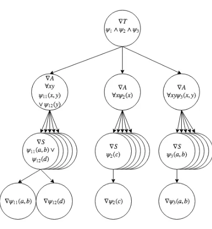
Figure 1.2: The flow of gradient through a sentence in an experimental setting. An arrow represents a partial derivative and shows how the gradient splits based on input dimensions. ∇T,∇Aand∇S are dependent on the instantiation and this images shows the importance of ∇T 6=0. The leaf nodes are not replicated in the last layer to unclutter the image.
We assume that some Gb(γ(ti)), i∈[o] is a function of p and continue forGb(γ(ti)).
∂Gb(γ(ti))
∂p =
∂Gb(l1(ti)∨ · · · ∨lm(ti))
∂p =
∂S(Gb(l1(ti)), . . . ,Gb(lm(ti)))
∂p =∇S·
∂Gb(l1(ti))
∂p
· · ·
∂Gb(lm(ti))
∂p
At this point we will stop but one can see how the partial derivatives could be taken w.r.t. a literal, which might contain a negation, and then take the partial derivative of the predicate as defined by either the LTN or the NTN. This shows us how∇T,∇A and ∇S are chained in order as can be seen in figure 1.2. We can also see that if ∇T = 0 then the gradient of the whole network will be0. Thus, we want to see if some of our operators have 0 gradient w.r.t. some input dimension or for some parts of the input domain. To make it clear, ∇T,
∇A and ∇S are dependent on the instantiation of RL and we want to see how the choice of many-valued functions impacts the gradient of our network.
Let us now compute the partial derivatives of the t-norms and start with the G¨odel t-norm.
∂TG(x1, . . . , xn)
∂xi
= ∂min(x1, . . . , xn)
∂xi
= (
1, ifxi= min(x1, . . . , xn)
0, otherwise
)
We can see that ∂TG(x1,...,xn)
∂xi is always 1 for a single xi (the minimum value). Thus, TG will
never have a zero gradient, as there is always a 1 along some dimension for all values of the input domain, i.e. ∇TG(x1, . . . , xn) 6= 0 for all x1, . . . , xn ∈ [0,1]10. Even though TG has a
10
non-zero gradient, it will only update parameters to one dimension at a time and in section 4.1 we argue that this can cause issues. Let us now explore partial derivative of the Lukasiewicz t-norm.
∂T L(x1, . . . , xn)
∂xi
= ∂max( Pn
j=1xj−(n−1),0)
∂xi
= (
1, if Pn
i=1xi> n−1
0, otherwise
)
We can see that ∂T L(x1,...,xn)
∂xi is 1 along all dimensions when
Pn
i=1xi > n−1, otherwise 0.
Essentially, the Lukasiewicz t-norm has 0gradient whenPn
i=1xi < n−1. This motivates the
following proposition.
Proposition 3 ( Lukasiewicz t-norm and input space). When the number of inputs tends to infinity and ∂T L(x1,...,xn)
∂xi 6=0 then
Pn i=1xi
n = 1.
Proof. If ∂T L(x1,...,xn)
∂xi 6= 0 then
Pn
i=1xi > n−1, given n > 0 then
Pn i=1xi
n > n−1
n we want
to know limx→∞
Pn i=1xi
n thus we use L’Hˆopital’s rule on n−1
n and when the number of input
parameters tends to infinity then
Pn i=1xi
n = 1, that is, the average value approaches 1.
This tells us that when the number of inputs approaches infinity and we want the gradient to be non-zero then the average value for each input approaches 1. At first, this might not seem like a big issue for us in the experimental setting, but in fact this is an issue withn= 2. Consider the case for n= 2, withx1 = 0.4 and x2 = 0.5, then the gradient will be 0. In our
experimental setting, all parameters of the network are initialized so that eachxi will have a
value close to 0, thus the gradient will always be0. We thus hypothesize that the Lukasiewicz t-norm will not be trainable in our experimental setting. We will revisit this hypothesis in section 2.4 in hypothesis 1.
Let us now compute the derivative of the product t-norm.
∂TP(x1, . . . , xn)
∂xi
= ∂ Qn
j=1xj
∂xi
=
n
Y
j=1∧j6=i
xj
We can see that if somexj = 0 then the partial derivative will be 0 to all variables but xj.
This does not cause much alarm for us, as in our experimental setting these values might be close to 0, but never actually 0. Again, we make note of the possible computational underflow issues.
We will not compute the partial derivatives of the s-norms, as they are very similar to the t-norms but we will address the issue of being ”easily satisfiable” we raised when introducing the Lukasiewicz s-norm.
Proposition 4 ( Lukasiewicz s-norm and input space). When the number of inputs tends to infinity and all xi >0 thenmin(Pni=1xi,1) = 1
Proof. Ifxi >0 then limn→∞Pni=1xi tends to infinity thus, min(limn→∞Pni=1xi,1) = 1
Lukasiewicz t-norm, due to the structure of our sentences, but it would be if we considered Disjunctive Normal Form instead of CNF. We will discuss the norms better in section 4.1.
Now similarly as we did with the norms, we want to compute the partial derivatives of the aggregation functions. For the minimum and maximum, we refer to the partial derivatives derived previously from the norms. That is, the gradient for Amin and Amax w.r.t. xi is
always 1 for a singlexi, the minimum and maximum value, respectively. For all other input
variables, it is 0. Let us now derive the partial derivative ofAari.
∂Aari(x1, . . . , xn)
∂xi
= ∂
Pn j=1xj
n
∂xi
= 1
n
We see thatAariw.r.t. xi has a constant gradient for every input over the whole domain, but
we notice that if the number of input variables tends to infinity then the gradient tends to0. Despite this drawback, we suspect thatAari will be the most practical in high dimensional
implementations due to the simplicity in computation, as it is a constant. Let us now derive the partial derivative ofAhar.
∂Ahar(x1, . . . , xn)
∂xi
=
∂Pnn j=1x
−1 j ∂xi = n x2 i( Pn
j=1x
−1
j )2
Similarly, the gradient for Ahar w.r.t. xi is always positive for every input over the whole
domain except when xi = 0 or all other xj = 0, j6=i, then it is not defined. Again, despite
these drawbacks, we are not too worried about these properties of theAhar and we will rely
heavily on it during experimentation.
We can also see that the partial derivative ofAowa w.r.t. xi iswi. This fact motivates the
hypothesis that in a high dimensional implementation the OWA operator might be useful by limiting computation over only the elements which are less satisfied. Thus, we hypothesize that an OWA operator which has 0 weights for the first elements and then distributes the re-mainder over the last elements will outperform the arithmetic mean in large-scale experiments and present this hypothesis in section 2.4 in hypothesis 8.
We will now address the issue of numerical underflow for the product norms. Instead of computing G(ϕ) we will compute log(G(ϕ)). Let us start by pointing to the fact that the log is a monotonically increasing function so the minimum of this function will also be the minimum of the log of this function. This implies that we can just as well search for optimal parameters of the log of the grounding, rather the grounding itself. Due to our sentence structure, we need to make sure that when we take the log of the conjunction, it is passed down, all the way to the disjunction. We start by considering the log-product t-norm.
Proposition 5 (The log-product t-norm). The log of the product t-norm is
log(TP(x1, . . . , xn)) = log( n
Y
i=1 xi) =
n
X
i=1
log(xi)
We can retrieve the product t-norm value from the log-product norm, TP(x1, . . . , xn) =
elog(TP(x1,...,xn)).
use it in the experimental setting to allow more numerically stable computation.
log(Ahar(x1, . . . , xn)) = log(
n
Pn
i=1x
−1
i
) = log(n)−log(
n
X
i=1 x−i 1)
= log(n)−log(
n
X
i=1
elog(x−i1)) = log(n)−log(
n
X
i=1
e−log(xi))
We will then use a numerically stable estimation for f(x1, . . . , xn) = log(Pni=1exi) in the
implementation.
Lastly, we consider the log of the product s-norm.
Definition 30 (The log-product s-norm). Thelog of the product s-norm is
log(SP(x1, . . . , xn)) = log(1− n
Y
i=1
(1−xi)) =log1p(−e
Pn
i=1log(1−xi))
Where log1p(x) = log(1 +x) is an optimized function for small x provided with many numerical computation libraries.
These derivations allow us to use the product norms in computation and in hypothesis 7 we will see the benefits of this extra work.
Experimental design
In this section, we describe how RL is used in the Semantic Image Interpretation (SII) task and how it will be evaluated. In section 2.1, we start by defining the task of SII and the dataset which is used to perform the task. In section 2.2, we define a knowledge base which describes the dataset along with logical properties of the dataset and define a grounding over this knowledge base allowing us to perform the SII task. In section 2.3, we define the measures used to evaluate classification performance and logical consistency of the model’s predictions. In section 2.4, we state our experimental hypotheses and motivate them.
2.1
The Setting
On a high level, the task of SII is to produce a scene graph given an image. In the scene graph, the nodes represent some object in the image and edges between nodes imply a relationship between the objects (Donadello et al., 2017; Serafini et al., 2017). The task is then to label objects and potential relations in the image. In addition to the image, we also base the predictions on background knowledge in the form of a knowledge base. The knowledge base describes properties about objects and relations in the image. We view the knowledge base as additional constraints and expect the predictions of the model to be consistent with these constraints.
We perform this task on the PASCAL-Part dataset (Chen et al., 2014) for the three following reasons. First, it provides a good selection of images along with bounding boxes around objects of interest in each image, its labelling and pair labellings. Second, a simple ontology is provided with the dataset which is easy to model in FOL. Third, a lot of work has already been done for this task on this dataset by Donadello et al. (2017); Serafini et al. (2017) which provides a good place to start.
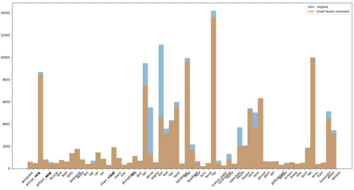
The PASCAL-Part dataset is a further annotated dataset of the PASCAL VOC 20101 dataset (Everingham et al., 2010). The original dataset contained 21,738 images (10,103 training, 9,637 testing) and 20 different classes for the classification task along with bounding boxes around objects of interests, but did not contain training data for relation prediction. This is added in the PASCAL-Part dataset, along with more fine-grained object classification. In fact, the object classification is so fine-grained that the parts are separated based on direction and alignment, f.ex. ”left leg” and ”right back upper leg”. We follow Donadello
1
PASCAL is an acronym for Pattern, Analysis, Statistical Modelling an Computational Learning and VOC is an acronym for Visual Object Classes.
et al. (2017); Serafini et al. (2017) by merging these finer partitions into a single partition, i.e. ”left leg” and ”right back upper leg” are taken as ”leg”. After making this adjustment there are 40 additional classes added to the dataset. These 40 classes are ”parts” of 20 original ”wholes”. For these classes we consider a single binary relation, the ”part of” relation for when ”x is a part of y”. The ontology provided states what ”parts” each ”whole” object consists of. As an example, in the dataset a ”bicycle” is considered as a whole consisting of the parts ”chain wheel”,”handlebar”, ”headlight”, ”saddle” and ”wheel”, thus ”saddle is a part of bicycle” is a true statement according to the ontology. Thus, when we classify something as a ”bicycle” and there is another object overlapping with ”bicycle” and that object is one of ”chain wheel”,”handlebar”, ”headlight”, ”saddle” and ”wheel” we are inclined to infer that these two are related. This is not always the case and in our experiments we want to know whether a particular ”saddle” is a part of a particular ”bicycle”, based on their representations. For practical reasons, these classes are then further separated into these three categories: indoor objects, vehicles and animals. The following experiments are only based on the PASCAL-Part training set (10,103 training examples) and we follow Donadello et al. (2017); Serafini et al. (2017) and eliminate images smaller than 6×6.
Figure 2.1: Class distribution of the training dataset. We can see that we have varying numbers of examples of each class. The image also shows the effect of removing images smaller than 6×6 from the dataset.
(a) In this image we can see the different class frequencies of an object in the ”part of” re-lation as a ”part”. All parts take part in the ”part of” relation.
[image:29.612.272.495.396.582.2](b) Similar to figure 2.3a, in this image we can see the different class frequencies of an object in the ”part of” relation as a ”whole”. All the wholes are ”bottle”, ”pottedplant”, ”tvmonitor”, ”chair”, ”sofa”, ”diningtable” but since ”chair”, ”sofa” and ”diningtable” do not have any parts they are never in the ”part of” relation.
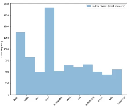
Figure 2.2: Class distribution over the training dataset with only indoor objects with small images removed. There are in total 11 classes.
Since the correct classification of classes impacts how well the ”part of” relation can be predicted, we are interested in learning more about this relation. For example, how sparse is the relation? That is, for all possible pairs of bounding boxes, how often are two bound-ing boxes related? Furthermore, what types of objects are most of-ten the ”wholes” and ”parts” in the ”part of” relation? We will use the ”indoor” objects dataset to answer these questions. See fig-ure 2.2 for the class distribution of the ”indoor” dataset. In the indoor dataset there are 2135 images bro-ken into 8535 bounding boxes, thus roughly 4 bounding boxes per im-age. There are in total 76037 pairs
of bounding boxes of which only 3049 are positive examples of the ”part of” relation or 4%. As we can see in figures 2.3a and 2.3b the class imbalance is not that dramatic when it comes to the ”part of” relation so we can treat each class equally and during training we will sample each class equally. In some settings, this might lead to overfitting for the class prediction but we see as a result of hypothesis 4 that this is not an issue and the class prediction generalizes well.
the images themselves as data, but rather use precomputed representations by Donadello et al. (2017). The representations are based on the output of a Fast R-CNN as well as additional hand-crafted features (Girshick, 2015). By using this representation we side-step the task of predicting bounding boxes in the image as well as computing representations of those bounding boxes. Predicting bounding boxes dynamically, using reasoning, sounds like a challenging task which we will not explore now. We want to know if RL can use logical constraints to improve binary classification, relation prediction and make the predictions logically consistent. We demonstrate that it can, by applying it directly to this representation, which is effectively the predictions of the Fast R-CNN.
2.2
The Models
In the following section, we will define a FOL language L in which we will describe the elements of PASCAL-Part dataset and logical constraints which apply to it. These FOL sentences are then considered as a knowledge base and we train the model to minimize the empirical loss of these sentences. During training we search for a partial groundingGbwhich is able to satisfy our knowledge base the most. The grounding is partial because the universal quantifiers are limited and 2147 constants withheld during training. Thus we optimize Gb w.r.t. to the training set and evaluate it on the withheld constants. During the experiments we observe that no Gb is able to satisfy the training dataset in the interval [1,1], or even [0.95,1], indicating that the model space is not expressive enough, that is, the representation, as well as the functions considered, cannot account for the data.
Let us now define a FOL L by defining a FOL signature which we use to describe a domain of bounding boxes. We let Btrain = {b1, . . . , b8525} be the training domain and
Btest ={b8526, . . . , b10672} be the testing domain, thus B = Btrain ∪Btest is the domain we
want to model and we refer to each bounding box with a constant symbol bi.
We model the object types as unary predicates P1 = {P1, . . . , P60} and the ”part of”
relation as a binary predicate P2 ={R}, thus P =P1∪ P2 ={P1, . . . , P60, R}. We will not
consider any function symbols for this task,F =∅. Thus, L=hC,P,∅i.
Before continuing and defining a groundingGover this language we need to discuss ground-ings of pairs of bounding boxes. In the following definition we follow Donadello et al. (2017); Serafini et al. (2017) and define groundings w.r.t. pairs of bounding boxes. This is not well defined for RL as RL defines groundings over the signature ofL. If we were to use the current definition of groundings and treat pairs as constants we will need to adjust the RL definition quite a lot to make it work. We rather consider an extension of RL which also considers pairs of constants as separate entities, that is, we assume that G(a, b), where a and b are constants, is a functionC × C →R2n+k where k≥0 and nis the dimension of grounding of
constants. We thus consider the possibility of adding extra dimensions to the representations when grounding pairs of constants. In the following paragraph we will define use this exten-sion to define a pair grounding. Lastly, when we consider the pairs,Bpairs ⊆B ×B we do
not consider all possible pairs of bounding boxes but rather only pairs derived from the same image, greatly reducing the number of possible pairs.
the box along with the top-right location (x2, y2). The grounding of a single bounding box
bi∈B is
G(bi) = (p(P1|bi), . . . , p(P60|bi), x1(bi), y1(bi), x2(bi), y2(bi))
As mentioned above, we don’t represent pairs just as the concetination of two representations of a bounding but we also add additional information in form of the inclusion ratioir(bi, bj)
for the pair of bounding boxes (bi, bj)∈Bpairs.
ir(bi, bj) =
area(bi∩bj)
area(bi)
G(bi, bj) = (G(bi),G(bj), ir(bi, bj), ir(bj, bi))
We then define the baseline we want to compare to also in terms of groundings, for each
j∈[|P1|]
Gb(Pj)(G(bk)) =
(
1 ifj = arg max|P1|
i=1 G(bk)i
0 o.w.
Where G(bk)i is the i-th dimension of the grounding for bounding box bk. Essentially, we
choose the type with the highest predicted value from the Fast R-CNN for each bounding box. For the ”part of” relation, we consider two baselines.
Gb1(R)(G((bi, bj))) =
(
1 ifir(bi, bj)≥th
0 o.w.
G2b(R)(G((bi, bj))) =
(
1 ifir(bi, bj)≥thand the resolved type of bi is ”part of”bj
0 o.w.
That is,G2
b(R) takes into account type compatibility.
The unary predicate baseline can either predict a special type of class, which has no positive examples in neither the training nor testing datasets, the ”background” class. This baseline will predict this class on a number of occasions, as this is what the Fast R-CNN will do. This will always lead to strictly worse performance. We will consider two baselines, one which predicts the ”background” class and another which will never predict this class. We do this to offer an additional comparison to our model, but essentially, our model will never predict this class.
Furthermore, the framework needs to be instantiated with some t-norm, s-norm, aggre-gation function and predicate implementations and in the following experiments we consider some combinations of these instantiations and denote them in the subscript;GLT N,har,TG(ϕ) refers to the LTN implementation of predicates, the harmonic mean as an aggregation op-erator and the G¨odel t-norm and s-norm. But since this notation is very verbose, we omit
LT N, har and TG from the notation, that is, G(ϕ) =GLT N,har,TG(ϕ) and when some other
t-norm is used instead, we indicate that using this notation. Thus,GLT N,har,T L(ϕ) is denoted asGT L(ϕ).
We have yet to define our knowledge base usingL which we want to satisfy. Recall that theempirical loss is defined w.r.t. h[v, w], ϕ(x)i ∈ K.
![Figure 1.1: The three t-norms; G¨odel, �Lukasiewicz and Product t-norm and their values along [0, 1] × [0, 1].Below the diagonal of the �Lukasiewicz it takes the value 0.](https://thumb-us.123doks.com/thumbv2/123dok_us/8382551.320991/13.612.108.486.109.235/figure-norms-lukasiewicz-product-values-diagonal-lukasiewicz-takes.webp)