Absolute performance of AUSGeoid09 in mountainous regions

Research Article

Vittorio Sussanna, Volker Janssen*, and Peter Gibbings

Absolute performance of AUSGeoid09 in

mountainous regions

Abstract: The Australian Height Datum (AHD) is the current national vertical datum for Australia, and AUS-Geoid09 is the latest quasigeoid model used to compute (normal-orthometric) AHD heights from Global Navigation Satellite System (GNSS) derived ellipsoidal heights. While previous studies have evaluated the AUSGeoid09 model across Australia, such studies have not focused on moun-tainous regions in particular. This paper investigates the performance of AUSGeoid09 in an absolute sense in the Mid Hunter and Snowy Mountains regions of New South Wales. Absolute (i.e. single point) comparisons were un-dertaken between AUSGeoid09-derived heights and pub-lished AHD heights. The performance of AUSGeoid09 was evaluated relative to its predecessor AUSGeoid98. In both study areas, an overall improvement is evident when ap-plying AUSGeoid09 to compute AHD heights in an abso-lute sense. In the Mid Hunter, AUSGeoid09 provided a sub-stantial improvement over its predecessor, clearly demon-strating the benefits of its new geometric component on GNSS-derived AHD height determination. In the Snowy Mountains, moderate improvement over AUSGeoid98 was evident. However, a slope was detected for AUSGeoid09 residuals, and it appears that the geometric component may have overcompensated for sea surface topography in this area. While this appraisal of AUSGeoid09 per-formance in mountainous regions is encouraging, it has been shown that some discrepancies still remain between AUSGeoid09-derived heights and AHD. Eventually, a new vertical datum will be necessary to ensure homogeneity across Australia.

Keywords: AUSGeoid09, AHD, geoid model, N _values,

height datum, GNSS

Vittorio Sussanna:Survey Infrastructure and Geodesy, NSW Land and Property Information, Sydney, Australia

*Corresponding Author: Volker Janssen:Survey Infrastructure and Geodesy, NSW Land and Property Information, Bathurst, Australia, E-mail: [email protected]

Peter Gibbings:Faculty of Health, Engineering and Sciences,

Uni-versity of Southern Queensland, Toowoomba, Australia

DOI 10.1515/jag-2014-0007

Received March 30, 2014; accepted July 04, 2014

1 Introduction

Mean Sea Level (MSL) is the surface that most countries have adopted as zero height for their national vertical da-tum [11, 17]. Heights above MSL are crucial information for a wide range of applications, e.g. flood modelling and emergency management. In Australia, MSL was approxi-mated as the basis of the Australian Height Datum (AHD), by setting to zero the average MSL values of 32 tide gauges around Australia for a period of about two years that began in 1966 [22].

More than 40 years later, it is well known that short-comings in the AHD realisation (AHD71 for mainland Aus-tralia and AHD83 for Tasmania) resulted in MSL not be-ing coincident with the geoid at the tide gauges involved. These shortcomings included not considering dynamic ocean effects (e.g. winds, currents, atmospheric pressure, temperature and salinity), a lack of long-term tide gauge data, and the omission of observed gravity. This has in-troduced considerable distortions of up to about 1.5 m into AHD across Australia, which is therefore considered a third-order datum [7, 21]. However, AHD continues to be a practical height datum that provides a sufficient approx-imation of the geoid for many applications. Consequently, in practice AHD heights are often accepted as being equiv-alent to orthometric heights.

N values (N), also known as geoid undulations or geoid-ellipsoid separations, can be used to convert GNSS-derived ellipsoidal heights (h) to AHD heights (H) and vice versa (providedN_andh_{refer to the same ellipsoid):}

H=h−N (1)

For many years, the use of geoid models (or quasigeoid models – see [23] for a discussion of the difference) has helped GNSS users to compute AHD heights from ellip-soidal heights. In the Australian context, AUSGeoid09 is the latest quasigeoid model that best fits AHD [1, 9].

While the performance of AUSGeoid09, along with the improvements it provides over its predecessor AUS-Geoid98, have been investigated previously [1, 18], these studies have not focused on mountainous regions. Consid-ering that gravity can change dramatically within a few kilometres on the earth’s surface in Australia [3], espe-cially in mountainous terrain, and that observed gravity data are generally sparse in these areas, it is necessary to evaluate mountainous regions in particular.

Geoid or quasigeoid models are commonly verified by using GNSS and orthometric height data. This can be done in an absolute and relative sense [6]: An ab-solute verification estimates the accuracy and precision of the (quasi)geoid, with respect to the geocentric ellip-soid, using GNSS networks that have been tied to an (in-ter)national reference frame and spirit-levelled orthome-tric heights that have been tied to the (national) vertical datum. A relative verification utilises GNSS-derived ellip-soidal height differences and spirit-levelled orthometric height differences to estimate the accuracy and precision of the (quasi)geoid gradients.

This paper investigates, from a user’s point of view, AUSGeoid09 performance in the mountainous regions of the Mid Hunter and the Snowy Mountains in New South Wales (NSW) in an absolute sense, using GNSS-derived el-lipsoidal heights and published AHD heights. A compari-son between AUSGeoid09 and its predecessor AUSGeoid98 is also performed in these two study areas.

2 AUSGeoid09

AUSGeoid09 was released in March 2011 by Geoscience Australia to replace the previous model AUSGeoid98 [8]. Both models refer to the GRS80 ellipsoid, which was adopted as the reference ellipsoid for the Geocentric Da-tum of Australia 1994 (GDA94), and cover the same geo-graphical area between 108◦E and 160◦E longitude and between 8◦_{S and 46}◦_{S latitude. However, AUSGeoid09 is}

provided as a 1’ by 1’ grid (approximately 1.8 by 1.8 km), making it four times denser than its predecessor [9].

Previous versions of AUSGeoid were predominantly gravimetric-only quasigeoids, and it was assumed that these were sufficiently close approximations of AHD – an assumption we now know to be incorrect. In contrast, AUSGeoid09 is a combined gravimetric-geometric quasi-geoid, providing a direct connection to AHD and thereby allowing a more reliable determination of AHD heights from GNSS observations [1]. The geometric component ac-counts for the offset between the gravimetric quasigeoid and AHD, which is predominantly caused by AHD not tak-ing into account sea surface topography includtak-ing the dif-ferential heating of the oceans.

Since the warmer or less dense water off northern Aus-tralia is about 1 metre higher than the cooler or denser wa-ter off southern Australia, AHD is about 0.5 m above the quasigeoid in northern Australia and roughly 0.5 m be-low the quasigeoid in southern Australia [1, 18]. The intro-duction of the geometric component takes care of most of this 1-metre trend across Australia (0.6-metre trend across NSW), thereby providing a better overall fit to AHD.

AUSGeoid09 has been shown to convert ellipsoidal heights to AHD heights with an accuracy of ±0.03 m (1 sigma) across most of Australia, with the exception of some pocket areas where the misfit can be larger than ±0.1 m due to errors caused by factors such as the age-ing levellage-ing network, geoid height variability or data defi-ciency [1]. Using a more practical approach, [18] found that AUSGeoid09 generally allows GNSS-based height determi-nation in NSW at the ±0.05 m level (1 sigma). In contrast, its predecessor AUSGeoid98 only provides an absolute ac-curacy of ±0.4 m [8, 10].

3 Absolute geoid model verification

Owing to the increased use of GNSS Continuously Oper-ating Reference Station (CORS) networks, the absolute ac-curacy of Nvalues is now more important than ever for AHD height determination using satellite positioning tech-niques [18]. In this paper, the performance of the AUS-Geoid09 model is verified in an absolute sense based on the comparison of a network of GNSS observations and published AHD heights. Using equation 1, AHD-derivedN

values (NAHD) are computed by subtracting the published

AHD height (HAHD) at each checkpoint from the ellipsoidal

These NAHD values are compared with N values

computed using AUSGeoid09 (and AUSGeoid98) with bi-linear, bi-quadratic, bi-cubic and bi-quartic interpolation to determine residuals (NAG–NAHD) for the following two

tests, both statistically and graphically [8]: – Comparison over all checkpoints. – Comparison as a function of AHD height.

Descriptive statistics are computed to obtain a numeri-cal representation of the population sample, as previously adopted by [1]. Z-statistics are employed to identify any outliers, in this paper defined as three times larger than the standard deviation. Since it is necessary to consider resid-uals of different signs, the Root Mean Square (RMS) is also utilised.

Generally speaking, the primary aim of this verifica-tion is to quantify the precision of AUSGeoid09 in regards to computing AHD heights at single points in mountainous regions and evaluate the four interpolation methods men-tioned above. Furthermore, a comparison between AUS-Geoid09 and its predecessor AUSGeoid98 is performed to quantify the expected improvement in mountainous areas.

4 Study areas and datasets

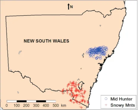
The absolute performance of AUSGeoid09 in mountainous regions is evaluated in two study areas located in NSW (Figure 1). Both study areas represent typical mountainous terrain conditions encountered in Australia and exhibit large differences in elevation. NSW Land and Property In-formation (LPI) provided two GNSS network datasets col-lected over many years, together encompassing 186 survey marks with known AHD heights of sufficient quality (Class C Order 3 or better) on public record in the Survey Control Information Management System (SCIMS). SCIMS is the state’s database containing about 250,000 survey marks across NSW, including coordinates, heights and other in-formation [19]. For a discussion of the terms class and or-der, the reader is referred to [15] and [5].

The Mid Hunter GNSS network adjustment covers an area of approximately 13,000 km2_{, stretching from about}

115 km south of the Mount Royal National Park to 170 km east of Mudgee. The terrain is mainly composed of valleys and mountains with elevations ranging between 20 m and 1,400 m. This dataset consists of 327 independent GNSS baselines observed between 147 marks. Of these, 82 SCIMS marks have known AHD heights (C3 or better), including 40 spirit-levelled marks of classification LCL3 or better.

Fig. 1.Location of the two study areas in NSW.

The Snowy Mountains GNSS network adjustment cov-ers an area of about 35,000 km2, approximately bounded in the north by Tumut and the ACT border to Cooma, and in the south by Albury and the Victorian border towards the coast. The terrain exhibits an undulated topography com-posed of mountains reaching a peak of 2,200 m and low valleys with elevations of about 200 m. The GNSS dataset consists of 629 independent baselines observed between 263 marks. Of these, 104 SCIMS marks have known AHD heights (C3 or better), including 94 spirit-levelled marks of classification LCL3 or better.

In total, across both study areas, this provides 186 checkpoints with known AHD heights of sufficient quality for a practical AUSGeoid09 performance verification in ab-solute terms and a comparison to AUSGeoid98. It should be noted that while some of the GNSS data used in this study contributed to the generation of AUSGeoid09, the datasets are considered sufficiently independent for the purpose of this study.

5 Data processing

The two GNSS networks used in this study were subject to several adjustments performed using the GeoLab least squares adjustment software. These adjustments were constrained to the national datum (GDA94) by holding sev-eral AUSPOS solutions [13] fixed, i.e. 7 and 27 marks in the Mid Hunter and Snowy Mountains networks respectively.

AUS-Geoid98 to enable comparison between the two models. The resulting GNSS-derived AHD heights are therefore in-dependent of published AHD heights.

Before computing any constrained least squares ad-justment (LSA), it was necessary to perform a minimally constrained LSA as per Surveyor General’s Direction No. 12 [20] and the ICSM Standards and Practices for Control Surveys (SP1), version 1.7 [15]. While it is acknowledged that a new version 2.0 of SP1 was released in late 2013 [16], this update does not affect the outcome of the analysis pre-sented in this paper. It is crucial to investigate the data quality before undertaking any comparison to ascertain the correct estimation of coordinate precision and estab-lish a realistic outcome of this research [10].

Ellipsoidal heights retrieved from AUSPOS solutions represent the vertical control marks that are held fixed throughout both the Mid Hunter and Snowy Mountains LSA networks. As outlined by [6], this constraint was nec-essary in order to connect the GNSS data to GDA94 and ob-tain a homogenous network of ellipsoidal heights for both study areas. This provided the basis for the comparison ofN_{values obtained from AUSGeoid09 and AUSGeoid98}

withNAHDvalues computed from published AHD heights

at the checkpoints.

Although the aim of this study was to verify the perfor-mance of AUSGeoid09 using the vertical component of the GNSS data, it was also important to evaluate the horizontal components because GeoLab computes the variance factor from a 3D adjustment and this provides further validation of the LSA results. In this fashion, the marks held fixed hor-izontally by LPI in the supplied adjustment datasets were adopted.

The static GNSS network observations were weighted based on an empirical method where the input stan-dard deviations of each GNSS baseline were computed using Northing-Easting (NE) correlations, as opposed to Northing-Easting-Up (NEU) correlations. While it is recog-nised that horizontal and vertical components are some-what correlated, this allowed the vertical component to re-main free for adjustment onto the ellipsoid.

The final outcome of the minimally constrained LSA established the method and path for the constrained LSA. In this case, the same empirical method of baseline weighting was adopted for both adjustments. Variance fac-tors for the horizontal and vertical components were com-puted separately, and several attempts were necessary to ensure that both variance factors were close to unity and passed the Chi-square test. The final estimation of pre-cision implemented for the constrained LSAs of the two study areas is summarised below.

Mid Hunter final weighting criteria (ppm values refer to baseline length):

– Horizontal: ±(0.007 m + 1.8 ppm) and ±0.0015 m cen-tring.

– Vertical: ±(0.005 m + 1.0 ppm), ±0.002 m antenna height measurement and ±0.012 m input standard de-viation for constrained stations.

Snowy Mountains final weighting criteria (ppm values re-fer to baseline length):

– Horizontal: ±(0.005 m + 1.0 ppm) and ±0.0015 m cen-tring.

– Vertical: ±(0.010 m + 1.0 ppm), ±0.002 m antenna height measurement and ±0.010 m input standard de-viation for constrained stations.

This method, however, does not identify any marginally detectable errors (i.e. small errors within the observations) because the Chi-square test is limited to verifying the net-work’s goodness of fit. In order to identify marginal er-rors, it was therefore necessary to evaluate the standard-ised residuals in conjunction with the redundancy values. The latter were computed by dividing the variance of the residual by the variance of the observation. It is recognised that redundancy values do not specifically detect a gross error, but they help identify marginally detectable errors.

Typical redundancy values for a GNSS network range between 0.5 and 0.8 [14]. The degree to which a residual would be affected by a marginally detectable error is com-puted by multiplying the redundancy value with the hypo-thetical gross error [2]. Hence, as redundancy values ap-proach unity, the influence of a gross error increases. Con-sidering a network, it follows that if a particular baseline returns a flagged standardised residual and a redundancy value is close to unity, a possibility exists that the base-line includes a marginally detectable error. Indeed, this method successfully identified the presence of marginally detectable errors in the Snowy Mountains dataset, and consequently four baselines were removed from the final LSA and two new baselines were added for redundancy.

Both the Mid Hunter and the Snowy Mountains net-works generated Class A surveys as per [15]. The ellip-soidal heights for the 104 checkpoints in the Snowy Moun-tains network displayed an average uncertainty of ±0.031 m at the 95% confidence interval (CI). The Mid Hunter net-work performed slightly better, resulting in an average un-certainty of ±0.024 m (95% CI) for the 82 checkpoints.

At each checkpoint,NAHDvalues were computed from

obtained from AUSGeoid09 and AUSGeoid98 using four different interpolation techniques.

6 Comparison over all checkpoints

The N _{values at the 186 checkpoints were computed}

four times, using linear, quadratic, cubic and bi-quartic interpolation, and then compared withN_values

derived from published AHD heights (NAHD). Descriptive

statistical analysis of the resulting AUSGeoid09N_values

showed that the differences between the four interpolation methods were negligible for the purpose of this research, withNvalues differing by only 1 or 2 mm between meth-ods. However, AUSGeoid98N_{values appear to be}

consis-tent only for bi-quadratic, bi-cubic and bi-quartic interpo-lation, while bi-linear interpolation providesN_{values that}

are up to about 7 mm different in some instances. The bet-ter consistency among different inbet-terpolation methods can be explained by the AUSGeoid09 model being four times denser than its predecessor. As a consequence, the remaing analyses presented in this paper utilise the bi-cubic in-terpolation method.

In order to examine the distribution of the residuals (NAG– NAHD), a Kurtosis test was performed. A negative

Kurtosis value indicates flatness with a large number of residuals concentrated along the side of a normal distribu-tion, while a positive value denotes a sample of a peak with the majority of the residuals concentrated in the proximity of the mean [4]. It was found that the AUSGeoid09 residu-als in both study areas are more consistent with a normal distribution with a large amount of residuals close to the mean, while AUSGeoid98 residuals denoted flatness with a large amount of residuals along the side of the normal distribution.

The comparison of the two quasigeoid models in the Mid Hunter study area shows a substantial improvement using AUSGeoid09 over its predecessor, evidenced by the standard deviation dropping from ±0.074 m to ±0.040 m. The RMS for AUSGeoid09 indicates an improvement fac-tor of 6 compared to AUSGeoid98. None of the two models indicate any outliers of three times their standard devia-tion.

As evident from Figure 2, the AUSGeoid98 residuals are heavily positive at around 0.25 m, while the AUS-Geoid09 residuals are well distributed around a near-zero mean. AUSGeoid09 provides an exceptional improvement over AUSGeoid98, showing no trends and exhibiting con-sistent residuals across the study area.

Fig. 2.Mid Hunter verification: Absolute residuals between quasigeoid-derived (AUSGeoid09 and AUSGeoid98)Nvalues and NAHDvalues for (a) increasing longitudes and (b) decreasing

south-ern latitudes.

Figure 2a suggests the existence of a slope in AUS-Geoid98 residuals in the longitudinal direction, dipping towards the east of the network, while Figure 2b indicates a rise in the middle of the study area’s latitudinal extent. The heavily positive AUSGeoid98 residuals are consistent with the geometric component of AUSGeoid09 generally amounting to about -0.2 m in this area [1], clearly showing the beneficial effect the introduction of the geometric com-ponent has on GNSS-derived AHD height determination in this area.

The comparison of the two quasigeoid models in the Snowy Mountains study area reveals a moderate improve-ment of AUSGeoid09 over AUSGeoid98 with the standard deviation dropping from ±0.090 m to ±0.070 m. However, no improvement was detected in the RMS. While neither model showed any outliers greater than three times the standard deviations, the mean of the residuals is closer to zero for AUSGeoid98 than AUSGeoid09 because the AUS-Geoid98 residuals are almost equally balanced between positive and negative values ranging between -0.224 m and 0.165 m. In contrast, the majority of AUSGeoid09 residuals are negative ranging from -0.284 m to 0.059 m.

Fig. 3.Snowy Mountains verification: Absolute residuals between quasigeoid-derived (AUSGeoid09 and AUSGeoid98)Nvalues and NAHDvalues for (a) increasing longitudes and (b) decreasing

south-ern latitudes.

Both models show a similar trend as a function of the latitudinal position, with residuals decreasing (smaller negative values) in the northern direction (Figure 3b). A closer evaluation of the residuals identifies that AUS-Geoid98 residuals are of larger magnitude and larger spread from the mean, while AUSGeoid09 residuals are more closely aligned with the mean, the only exception being two checkpoints at latitude -37.0◦ (and longitude 149.9◦). If these two residuals are removed, the range in AUSGeoid09 residuals decreases by about 75 mm and the standard deviation improves to ±0.065 m. However, there is not enough evidence supporting a gross error within these two checkpoints to justify their removal.

Figure 3 shows that a slope is evident within AUS-Geoid09 residuals from the north-west to the south-east corner, with the majority of negative residuals situated at the south-east corner of the study area. This direction is perpendicular to the known general south-west to north-east slope present in the gravimetric component of AUS-Geoid09 (and more generally the geoid across Australia). While this slope indicates that a small residual geomet-ric effect may be present in this area, the sample is not large enough to identify any anomalies in AUSGeoid09 with any certainty. The small offset between the two mod-els is consistent with the geometric component of AUS-Geoid09, generally amounting to about -0.1 m or less in this area [1]. This suggests that the geometric component of AUSGeoid09 may have overcompensated for the effect of sea surface topography in this case.

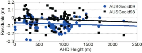
Fig. 4.Mid Hunter verification: Absolute residuals between quasigeoid-derived (AUSGeoid09 and AUSGeoid98)Nvalues and NAHDvalues as a function of AHD height.

Fig. 5.Snowy Mountains verification: Absolute residuals between quasigeoid-derived (AUSGeoid09 and AUSGeoid98)Nvalues and NAHDvalues as a function of AHD height.

7 Comparison as a function of AHD

height

In mountainous regions, it is useful to investigate the per-formance of the two quasigeoid models as a function of AHD height. While it is recognised that the sample of checkpoints decreases considerably with increasing ele-vation, this will provide an indication of how well the two models fit AHD in undulating terrain. Following the approach taken by [8], Figure 4 illustrates the absolute

N_{value residuals for both quasigeoid models as a}

func-tion of AHD height for the 82 checkpoints located in the Mid Hunter study area. Figure 5 shows the corresponding results for the 104 checkpoints in the Snowy Mountains study area.

Table 1.Mid Hunter verification: Descriptive statistics of the absolute residuals between AUSGeoid09Nvalues andNAHDvalues.

AHD No. of Min Max Mean Range STD RMS Height (m) Points (m) (m) (m) (m) (m) (m)

>20 82 -0.134 0.109 -0.014 0.243 0.040 0.042

>200 54 -0.134 0.109 -0.009 0.243 0.046 0.045

>400 22 -0.134 0.109 -0.002 0.243 0.059 0.058

>600 13 -0.085 0.109 0.018 0.194 0.055 0.055

>800 6 -0.085 0.109 0.033 0.194 0.069 0.071

>1,000 3 0.056 0.109 0.083 0.053 0.026 0.086

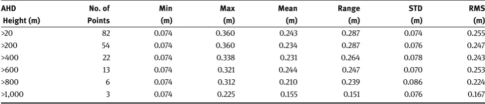
Table 2.Mid Hunter verification: Descriptive statistics of the absolute residuals between AUSGeoid98Nvalues andNAHDvalues.

AHD No. of Min Max Mean Range STD RMS Height (m) Points (m) (m) (m) (m) (m) (m)

>20 82 0.074 0.360 0.243 0.287 0.074 0.255

>200 54 0.074 0.360 0.234 0.287 0.076 0.247

>400 22 0.074 0.338 0.231 0.264 0.078 0.243

>600 13 0.074 0.321 0.244 0.247 0.070 0.253

>800 6 0.074 0.312 0.210 0.239 0.086 0.224

>1,000 3 0.074 0.225 0.155 0.151 0.076 0.167

again demonstrates the benefit of introducing the geomet-ric component, but also indicates that it may have over-compensated for the sea surface topography effect in the Snowy Mountains study area. However, it should be noted that these results are not a true representation of a contin-uous elevation model because the checkpoints are located across a large area and both datasets contain a small num-ber of checkpoints at the higher elevations.

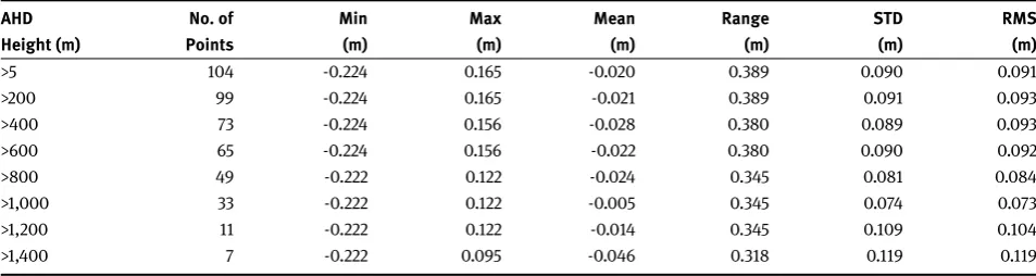
These findings are supported by investigating descrip-tive statistics of the absolute residuals, calculated for all checkpoints in increments of 200 m in AHD height. Table 1 and Table 2 show the statistics of the Mid Hunter study area, while Table 3 and Table 4 present the statistics of the Snowy Mountains dataset for the AUSGeoid09 and AUS-Geoid98 models, respectively.

In the Mid Hunter study area, both quasigeoid models demonstrate relatively stable and consistent sets of statis-tics with increasing elevation. AUSGeoid09 shows sub-stantial improvements in the mean, standard deviation, RMS and also the range of residuals. The large positive bias in the mean of the AUSGeoid98 residuals has been success-fully accounted for by AUSGeoid09.

In the Snowy Mountains study area, AUSGeoid09 shows improvements over AUSGeoid98 in terms of stan-dard deviation and range, particularly for higher eleva-tions. The AUSGeoid09 statistics are also generally more stable with increasing elevation. However, the RMS only shows improvement for the highest elevations. As

men-tioned earlier, the mean of the AUSGeoid09 residuals is no-ticeably biased to the negative.

8 Concluding remarks

By examining two datasets located in New South Wales, this paper has investigated the performance of the AUS-Geoid09 quasigeoid model in mountainous regions and compared it to its predecessor AUSGeoid98 from a user’s perspective, in an absolute sense. The differences between the four interpolation methods examined (i.e. bi-linear, bi-quadratic, bi-cubic and bi-quartic) were negligible for AUSGeoid09, while AUSGeoid98 showed some inconsis-tencies when using bi-linear interpolation. AUSGeoid09 has demonstrated increased consistency and accuracy compared to its predecessor, owing to the inclusion of a geometric component, a larger amount of input data and its higher density. However, this improvement was more evident in the Mid Hunter than in the Snowy Mountains.

posi-Table 3.Snowy Mountains verification: Descriptive statistics of the absolute residuals between AUSGeoid09Nvalues andNAHDvalues.

AHD No. of Min Max Mean Range STD RMS Height (m) Points (m) (m) (m) (m) (m) (m)

>5 104 -0.284 0.059 -0.076 0.343 0.070 0.103

>200 99 -0.284 0.059 -0.077 0.343 0.071 0.104

>400 73 -0.209 0.051 -0.091 0.260 0.059 0.108

>600 65 -0.209 0.051 -0.091 0.260 0.060 0.108

>800 49 -0.209 0.051 -0.090 0.260 0.066 0.111

>1,000 33 -0.195 0.051 -0.074 0.246 0.057 0.093

>1,200 11 -0.112 0.051 -0.023 0.163 0.051 0.054

>1,400 7 -0.112 0.051 -0.016 0.163 0.051 0.050

Table 4.Snowy Mountains verification: Descriptive statistics of the absolute residuals between AUSGeoid98N_{values and}NAHDvalues.

AHD No. of Min Max Mean Range STD RMS Height (m) Points (m) (m) (m) (m) (m) (m)

>5 104 -0.224 0.165 -0.020 0.389 0.090 0.091

>200 99 -0.224 0.165 -0.021 0.389 0.091 0.093

>400 73 -0.224 0.156 -0.028 0.380 0.089 0.093

>600 65 -0.224 0.156 -0.022 0.380 0.090 0.092

>800 49 -0.222 0.122 -0.024 0.345 0.081 0.084

>1,000 33 -0.222 0.122 -0.005 0.345 0.074 0.073

>1,200 11 -0.222 0.122 -0.014 0.345 0.109 0.104

>1,400 7 -0.222 0.095 -0.046 0.318 0.119 0.119

tion of the checkpoints, and relatively stable and consis-tent sets of statistics were obtained for increasing eleva-tions. AUSGeoid09 has clearly demonstrated the benefit of its geometric component on GNSS-derived AHD height de-termination in this area.

In the Snowy Mountains study area, AUSGeoid09 pro-vided moderate improvement over AUSGeoid98, with the standard deviation dropping form ±0.090 m to ±0.070 m. However, it should be noted that the majority of AUS-Geoid09 residuals were negative, rather than evenly dis-tributed around a zero mean. This suggests that the geo-metric component of AUSGeoid09 may have overcompen-sated for sea surface topography in this case. The dataset also detected a slope in AUSGeoid09 residuals from the north-west to the south-east corner, indicating that a small residual geometric effect may be present in this area. How-ever, the sample size is not sufficiently large to identify any anomalies in AUSGeoid09 with any certainty. It is recog-nised that the terrain correction (TC) is likely to represent a more prominent error source for theNvalues in this study area. The accuracy of its computation is dependent on the integrity of the Digital Elevation Model (DEM) in the re-gion, and for the rugged terrain of the Snowy Mountains

this TC element is expected to show a larger degree of un-certainty than in the Mid Hunter.

It is important to note that this investigation of abso-lute AUSGeoid09 performance in the two study areas does not provide a general verification of AUSGeoid09 in other mountainous regions. It is acknowledged that sources of error exist within extensive datasets, even after careful in-vestigation. Furthermore, GNSS and AHD height data have their own error budgets, and the sparseness of gravity data and any uncorrected biases in the spirit-levelling data in mountainous terrain may have contributed to some of the trends shown. Consequently, the results presented cannot be relied upon as an exact indication of the accuracy and precision of AUSGeoid09. However, considering that the main use of AUSGeoid09 is to compute AHD heights from GNSS-derived ellipsoidal heights, the data and method employed in this paper represent the most practical means of absolute quasigeoid verification currently available.

ar-eas have shown. Eventually, the introduction of a new na-tional vertical datum for Australia will be necessary in or-der to achieve higher consistency and generate a verti-cal reference surface that is more closely aligned with the geoid. For a discussion of possible options in this regard, the reader is referred to [12].

References

[1] Brown N. J., Featherstone W. E., Hu G., Johnston G. M., AUS-Geoid09: A more direct and more accurate model for converting ellipsoidal heights to AHD heights,Journal of Spatial Science

56(1), (2011), 27-37.

[2] Caspary W. F., Concepts of network and deformation analysis (3rd ed.). Sydney, Australia, University of New South Wales, 1987.

[3] Darbeheshti N., Featherstone W. E., Non-stationary covariance function modelling in 2D least-squares collocation,Journal of Geodesy83(6), (2009), 495-508.

[4] DeCarlo L. T., On the meaning and use of Kurtosis, Psychologi-cal Method2(3), (1997), 292-307.

[5] Dickson G., Control surveys: Why things are the way they are and not the way you think they should be! Proc. Association of Public Authority Surveyors Conference (APAS2012), 19-21 March, Wollongong, Australia, 12-28, 2012.

[6] Featherstone W. E., Absolute and relative testing of gravimetric geoid models using global positioning system and orthometric height data,Computers and Geosciences27(7), (2001),

807-814.

[7] Featherstone W. E., Filmer M. S., The north-south tilt in the Australian Height Datum is explained by the ocean’s mean dy-namic topography,Journal of Geophysical Research117, (2012),

C08035, doi:10.1029/2012JC007974.

[8] Featherstone W. E., Guo W. Evaluations of the precision of AUS-Geoid98 versus AUSGeoid93 using GPS and Australian Height Datum data,Geomatics Research Australasia74, (2001), 75-102.

[9] Featherstone W. E., Kirby J. F., Hirt C.et al., The AUSGeoid09

model of the Australian Height Datum,Journal of Geodesy85(3),

(2011), 133-150.

[10] Featherstone W. E., Kirby J. F., Kearsley A. H. W.et al._{, The}

AUSGeoid98 geoid model of Australia: Data treatment, com-putations and comparisons with GPS-levelling data,Journal of Geodesy75(5-6), (2001), 313-330.

[11] Featherstone W. E., Kuhn M., Height systems and vertical da-tums: A review in the Australian context,Journal of Spatial Sci-ence_{51(1), (2006), 21-41.}

[12] Filmer M. S., Featherstone W. E., Three viable options for a new Australian vertical datum,Journal of Spatial Science_57(1),

(2012), 19-36.

[13] GA. AUSPOS - Online GPS Processing Service (accessed July 4, 2014, at http://www.ga.gov.au/earth-monitoring/geodesy/ auspos-online-gps-processing-service.html).

[14] Harvey B. R., Practical least squares and statistics for survey-ors. Monograph 13 (3rd ed.), Sydney, Australia, University of New South Wales, 2009.

[15] ICSM. Standards and practices for control surveys (SP1), ver-sion 1.7, 2007.

[16] ICSM. Standard for the Australian survey control network (SP1), version 2.0, 2013.

[17] Janssen V., Understanding coordinate reference systems, da-tums and transformations,International Journal of Geoinformat-ics_{, 5(4), (2009), 41-53.}

[18] Janssen V., Watson T., Improved AHD71 height determination from GNSS using AUSGeoid09 in New South Wales, Australia,

Journal of Global Positioning Systems9(2), (2010), 112-121.

[19] Kinlyside D., SCIMS3: The next generation Survey Control In-formation Management System. Proc. Association of Public Authority Surveyors Conference (APAS2013), 12-14 March, Can-berra, Australia, 174-186, 2013.

[20] LPI. Surveyor General’s Direction No. 12 (accessed July 4, 2014, at http://www.lpi.nsw.gov.au/surveying/publications/ surveyor_generals_directions).

[21] Morgan P., An analysis of the Australian Height Datum 1971,

Australian Surveyor_{37(1), (1992), 46-63.}

[22] Roelse A,. Granger H. W., Graham J. W., The adjustment of the Australian levelling survey 1970-1971. Technical Report 12, Canberra, Australia, Division of National Mapping, 1971. [23] Vaniček P., Kingdon R., Santos M., Geoid versus quasigeoid: A