Models of the Polymodal Provability Logic
MSc Thesis
(
Afstudeerscriptie
)
written byThomas F. Icard, III
(born March 12, 1984 in Florida, USA)
under the supervision of Lev D. Beklemishev andDick de Jongh, and submitted to the Board of Examiners in partial fulfillment of the requirements
for the degree of
MSc in Logic
at theUniversiteit van Amsterdam.
Date of the public defense: Members of the Thesis Committee:
August 15, 2008 Lev D. Beklemishev
Contents
1 Introduction 2
1.1 GLandGLP. . . 2
1.1.1 Classical Provability Logic . . . 2
1.1.2 From Provability toω-Provability to Reflection Principles 4 1.2 GLPand Ordinal Analysis . . . 6
1.3 Outline of the Thesis . . . 7
2 Relational Models 8 2.1 Frame Incompleteness . . . 8
2.2 Models of GLP. . . 9
2.2.1 The LogicJ. . . 10
2.2.2 Beklemishev’s Blow-up Models . . . 13
2.3 Ignatiev’s Frame U . . . 18
2.4 Words and Ordinals . . . 25
3 The Canonical Frame of GLP0 28 3.1 Descriptive General Frames . . . 29
3.1.1 Basic Facts . . . 29
3.1.2 Descriptive Frames and Canonical Frames . . . 30
3.2 The FrameVc . . . . 32
3.2.1 Compactness . . . 32
3.2.2 Tightness . . . 35
4 Topological Models 37 4.1 Ordinal Completeness of GLP0 . . . 38
4.1.1 The Space Θ . . . 38
4.1.2 Limit Points in Θ . . . 42
4.2 GLP-Spaces . . . 43
1
Introduction
Arguably, the most successful applications of modal logic to other areas of math-ematics have been the so called “provability” interpretations, and various topo-logical interpretations.1 This thesis concerns both of these interpretations, al-beit each only indirectly. The Polymodal Provability Logic known asGLPhas held significant interest in the study of strong provability predicates in arith-metical theories, as well as in the study of ordinal notation systems for these theories. In particular, the closed fragment of GLP, which we shall denote
GLP0, simply GLP restricted to the language without variables, has found applications in mainstream proof theory (See Section 1.2). The majority of this thesis is therefore dedicated to exploring relational and topological models of this logic. At the same time, however, an underlying impetus for this study is the fact that the full logicGLPwith variables is frame-incomplete (See Section 1.1.2). While a thorough treatment of the full logic is beyond the scope of the thesis, it is hoped that a better understanding of the closed fragment, and in particular the interaction between relational and topological interpretations of the closed fragment, will shed some light on the full fragment. Last but not least, some of the structures we will come across are sufficiently intriguing and natural, we believe, so as to merit interest in and of themselves.
1.1
GL and GLP
1.1.1 Classical Provability Logic
The idea of a logic of provability goes back to a short paper by Kurt G¨odel ([G¨odel, 1933]). LetB(x, y) be (any reasonable variation of) G¨odel’s ∆0 predi-cate formalizing, “y is the code of a proof in Peano Arithmetic of the sentence with G¨odel numberx,” with Bew(x) =∃yB(x, y), and letA# be the numeral of the G¨odel code ofA. G¨odel first showed that the following schema is valid:
Bew((A→B)#)⇒(Bew(A#)⇒Bew(B#))
In fact, not only is the schema true, it can be proven in Peano Arithmetic (henceforthPA) itself, whereby the meta-conditional “⇒” becomes “→” in the language of arithmetic. The following rule also holds for allA (as an instance of so called Σ1-completeness):
IfAis provable, thenBew(A#) is provable.
This fact is also formalizable inPA(by so called provable Σ1-completeness), so we have one more schema:
Bew(A#)→Bew(Bew(A#)#)
Ignoring the distinction between a formula and its G¨odel number, and replacing
Bewwith ¤, we can write each of these schemas and rules in what looks like the standard modal language, giving each a name suggestive thereof.
K: ¤(φ→ψ)→(¤φ→¤ψ)
4: ¤φ→¤¤φ
And the rule,
Nec: Ifφ, then¤φ.
If we add to this the rulemodus ponens, we obtain the modal systemK4. Later, building on work by Hilbert and Bernays, Martin L¨ob identified ([L¨ob, 1955]) one last principle that he showed is sufficient, given the other axioms, for a schematic proof of G¨odel’s Second Incompleteness Theorem. The extra principle is known as L¨ob’s Axiom (stated here in the anachronistic modal language):
L: ¤(¤φ→φ)→¤φ
The resulting extension of K4 is called GL (named after G¨odel and L¨ob). Essentially what G¨odel, L¨ob, and Hilbert and Bernays showed is that if φ is a theorem of GL, then for all functions f that send propositional variables to arbitrary arithmetical formulas, ¤ψ to Bew(ψ#), and that commute with boolean operations, f(φ) is a theorem of PA. And this is indeed enough to prove the Second Incompleteness Theorem using purely modal reasoning: If PA could prove its consistency statement, ¬¤⊥, then ¤⊥ → ⊥would follow. By rule Nec, we would have ¤(¤⊥ → ⊥), and finally by Axiom L and one application ofmodus ponens, ¤⊥, that is,PA would be inconsistent.
The question eventually arose whether GLencompasses all schemata prov-able of the provability predicate. Provoked by a notice to the American Mathe-matical Society written by George Boolos, Robert Solovay provedGLis arith-metically complete.2
Theorem 1.1.1 ([Solovay, 1976]). GL⊢φiff PA ⊢f(φ), for allf.
The logic GL is sound and complete with respect to the class of finite, rooted, partially ordered Kripke frames (henceforthGL-frames), a result first published by Krister Segerberg ([Segerberg, 1971]). The basic idea of Solovay’s proof is to embed an arbitraryGL-model into Peano Arithmetic, so that any refuting Kripke model becomes an arithmetical counterexample.
This striking correspondence between modal logic and arithmetic opened up the possibility of proving interesting arithmetical results using purely modal methods, one of the most famous examples being the de Jongh-Sambin Fixed Point Theorem (in fact proven even before the publication of Solovay’s paper), which shows when and why certain formulas have explicit and unique solutions, thus generalizing the original fixed point theorem. For, in a very definite sense,
GLtells us everything there is to know about what a reasonable arithmetical theory can say about the behavior of its own provability predicate.
2Solovay also proved that the non-normal logicGLS, obtained by extending GL with
1.1.2 From Provability to ω-Provability to Reflection Principles
G¨odel’s original proofs of the incompleteness theorems did not apply to all consistent arithmetical theories, but merely to theories that wereω-consistent. Recall thatTisω-inconsistent if there is an arithmetical formulaA(x) such that, T⊢ ∃xA(x), but for each natural number n,T ⊢ ¬A(n).3
T is ω-consistent if it is not ω-inconsistent. ω-consistency is stronger than consistency: If T is
ω-consistent, then there is some formula that T does not prove (either ¬A(n) for somen, or ∃xA(x), for every predicate A(x)), so it is certainly consistent; however, there are examples of consistent theories that are notω-consistent (e.g. add the sentenceBew(0=1) toPA). And it was not until later that John Rosser extended the range of incompleteness to consistent theoriestout court.
We sayAisω-provablein a theoryT, if the theoryT+¬Aisω-inconsistent.4 Asω-consistency implies consistency, so also ω-provability implies provability: If A is not provable, then T + ¬A is consistent, i.e. not inconsistent, hence not ω-inconsistent, and so A is not ω-provable. George Boolos was the first to address the logic of ω-provability for PA([Boolos, 1980]). He found that it is also GL, and with some minor adjustments the Solovay-style arithmetical completeness proof can be used.
The next natural question was to determine the joint logic of provability andω-provability so as to capture the exact relationship between them. Several principles we can see right away must be valid. Let us write [0] for normal provability and [1] for the natural arithmetical formalization of ω-provability as a Σ3-predicate. We know both [0] and [1] satisfy all of the axioms of GL. Moreover, by our earlier observation, we obviously have,
[0]φ→[1]φ
It is also not difficult to see that this principle should also be part of the logic:
¬[0]φ→[1]¬[0]φ
Reasoning in PA, suppose A is not provable. Then no number n is the code of a proof of A, that is, ¬B(n, A#) is true for all n, which means that PA
⊢ ¬B(n, A#) for alln. But then it is easy to see thatPA+∃xB(x, A#) will be
ω-inconsistent, that is to say, ¬∃xB(x, A#) is ω-provable. And ∃xB(x, A#) is exactly the definition ofBew(A#), so¬Bew(A#) isω-provable.
Giorgi Japaridze was the first to prove that these principles are indeed suf-ficient ([Japaridze, 1985]). The proof is a non-trivial variation on Solovay’s method for proving arithmetical completeness of GL.
In a certain sense, the set of ω-provable sentences of PA gets us one step closer to the set oftrue arithmetical sentences than the set of normally provable sentences. This can be better seen by considering an alternative, but equivalent,
3For convenience, we use bold notation for the arithmetical representation of numerals and
logical symbols.
4The presentation in this section is very much based on that in [Boolos, 1993]. This is also
formulation ofω-provability. Let us sayAis provable by one application of the
ω-rule if there is some formula B(x) such thatPA ⊢B(n) for all n, andPA ⊢ ∀xB(x)→A. It is easy to see that these two concepts coincide. That provability by one application of theω-rule impliesω-provability is obvious. For the other direction, ifAisω-provable, there is someB(x) such that (using the Deduction Rule), for alln,PA ⊢ ¬A→ ¬B(n), but PA⊢ ¬A → ∃xB(x). It follows that, PA ⊢ ∀x(¬A → ¬B(x))↔ ⊥, and in particularPA ⊢ ∀x(¬A→ ¬B(x))→A. SoA is provable by one application of theω-rule.
Taking provability by one application of theω-rule as an alternative defini-tion of ω-provability, this notion naturally gives rise to a whole succession of stronger and stronger provability predicates. We could then let [2] correspond to the formalization ofprovable by two applications of theω-rule, and so on for all natural numbers. In this way, adding more and more sentences to this list of “provable” formulas, we gradually approach the standard model of all true arithmetical sentences, since infinitely many applications of the rule gives all such sentences. Obviously the logic of “n-provability” for each n will mirror that of normal provability, just as 1-provability does. And the relationship be-tweenn- andn+ 1-provability is analogously captured by that between 0- and 1-provability. Thus, we are ready to give the formal definition of GLP(Pfor “polymodal”):
Definition 1.1.2. The logicGLPis defined by the following axioms, forn < ω:
(i) All tautologies
(ii) [n](φ→ψ)→([n]φ→[n]ψ)
(iii) [n]([n]φ→φ)→[n]φ
(iv) hniφ→[n+ 1]hniφ
(v) [n]φ→[n+ 1]φ
GLPis closed under modus ponens, and [n]-necessitation for alln < ω.
As in the case of GL, we put a natural restriction on the functions f from modal formulas to arithmetical formulas, in particular so that, e.g. [n]φ is always mapped to the formalization of “φis provable by napplications of the
ω-rule.” Then, Japaridze’s Theorem can be stated:
encompassed by the more general and canonical notion ofreflection principles, sentences of the form,
Bew(A#)→A
When such principles are restricted to subclasses of the arithmetical hierarchy, a more natural definition ofn-provability arises.
WhereThΠn(N) is the set oftrueΠnarithmetical sentences, let us say a
the-oryTisn-consistent ifT+ThΠn(N) is consistent, otherwise it isn-inconsistent.
It is known that the statement of a theory’sn-consistency is equivalent (prov-ably in a weak arithmetic) to Σn-reflection over that theory. And a natural notion ofn-provability of a sentence can be defined analogously to the case of
ω-provability:
A sentenceAisn-provable inTif the theory T+¬Aisn-inconsistent.
Son-provability becomes a natural Σn+1 predicate meaning, “provable fromT along with all true Πn sentences,” and the connection to reflection principles thereby becomes more evident.5
Theorem 1.1.3 was extended by Konstantin Ignatiev ([Ignatiev, 1993]) to a wider class of possible interpretations of [n]φ. He isolated minimal requirements for an interpretation to give rise toGLP, andn-provability turns out to be the weakest possible. All of these considerations together suggest thatn-provability takes precedence as the standard arithmetical interpretation of GLP. The ap-plication discussed in the next section strengthens this suggestion yet further.
1.2
GLP and Ordinal Analysis
One of the traditional aims of proof theory has been to assign appropriate ordinals to arithmetical theories. By appropriate, it is meant, on the one hand, that the assignment should provide a comparative measure of “strength” of different theories, most notably consistency strength. On the other, it should be possible to glean computational information about such theories from their respective ordinals, e.g. a characterization of the class of functions the theory is able to prove total. Ordinal analysis began with Gerhard Gentzen, who proved that Peano Arithmetic is consistent by using induction up to the ordinal ǫ0, that is, the least ordinal fixed point of the equation ωα = β. In the same paper, Gentzen showed that PA is able to verify transfinite induction for any arithmetical predicate up to any ordinal less thanǫ0. Thus, a reasonable idea for the definition of theproof-theoretic ordinalof a theoryTcould be something like, “the least ordinal needed to prove the consistency ofT,” or else, “the supremum of the ordinals (order types) thatTis able to prove are well-founded.”
The problem with these definitions is that pathologies creep in where details, such as how ordinals are to be represented in the theory, are left vague and open-ended. For instance, Georg Kreisel has shown that it is possible to define a (primitive recursive) ordering of typeω so that even very weak theories can prove the consistency of quite strong theories, likePA, using induction on this
ordering. As a converse to this, Lev Beklemishev has shown that for any ordinal
λ < ωCK
1 there is a (primitive recursive) well-order of order typeλsuch that no sufficiently modest theory can prove the consistency ofPA, even with transfinite induction up to λ.6 One lesson that could be drawn from such examples is that the notion of a proof-theoretic ordinal should abstract away as much as possible from the particular syntactic details of the theory in question, and that the assignment of an ordinal should be somehowcanonical. The problem then becomes, what sort of informationshould be relevant to determining a theory’s ordinal? And what exactly does, or should,canonical mean here?
In [Beklemishev, 2004a], Beklemishev proposes that the relevant information is captured, roughly, by the logic GLP. More particularly, he considers the Lindenbaum-Tarski Algebra of GLP (See Definition 3.1.10), in which terms corresponds to polymodal formulas and the identities are exactly the theorems of GLP. On the 0-generated free subalgebra, corresponding exactly to the set of closed formulas of GLP, a primitive recursive relation<0is defined:
φ <0ψ ⇔ GLP⊢ψ→ h0iφ
As we shall see later in this thesis (Section 2.3), the order type of<0 is exactly
ǫ0whenTis a sound arithmetical theory. Given the arithmetical interpretation ofGLPasn-provability, a direct connection can be made betweenn-provability and quantifier complexity. Finally, by defining a bijection between elements of this algebra and ordinals less thanǫ0(see Definition 2.4.4), an ordinal notation system is established that essentially depends only on the natural quantifier complexity levels of the arithmetical language. This treatment allows for a very simple, and “high-level” proof of Gentzen’s result on the consistency of PA, as well as a more refined ordinal analysis of theories weaker thanPA.
As this seems to be a promising and attractive approach to one of the central problems in proof theory and mathematical logic generally, the closed fragment of GLP, and the associated modal algebra, holds special interest.
1.3
Outline of the Thesis
The thesis is divided into three main sections. In the first section, we investigate relational models of GLP. After presenting a simplified treatment of Beklem-ishev’s blow-up model construction, we exploit completeness for such models to obtain a new, purely semantic proof thatGLP0 is complete with respect to Ignatiev’s universal frame U. Following this, we investigate formula definable subsets ofU in anticipation of our work in the next two sections.
In the second section, we explore the connection between the frameUand the canonical frame of GLP0. Using the theory of descriptive frames, we extend
U to a frame Vc that is isomorphic to the canonical frame, thus obtaining a detailed definition of this object in terms of a coordinate structure we develop in Section 2.
6Recall thatωCK
1 is the least ordinal that cannot be represented as the order type of a
Finally, in the last section, we explore topological models of GLP. The central result of this section is an analog of the Abashidze-Blass Theorem for
GL, to the effect thatGLP0 enjoys topological completeness with respect to a simply defined polytopology on the ordinal ǫ0+ 1. This space can be seen as a condensed, and much simplified, version of the canonical frame of GLP0. We then consider the possibility of an extension of this theorem to fullGLP. However, such an extension would require large cardinal assumptions beyond ZFC, so we leave this further question for future work.
2
Relational Models
2.1
Frame Incompleteness
GLPis the normal polymodal logic defined as follows:
Definition 2.1.1 (The Logic GLP).For eachn < ω, extendKby the axioms:
(iii) [n]([n]φ→φ)→[n]φ
(iv) hniφ→[n+ 1]hniφ
(v) [n]φ→[n+ 1]φ
As usual, we would like to know what class of frames, if any, this logic defines. Unfortunately, in this case, the answer is that there is no single frame on whichGLPis sound. Recall the relational semantics of GL:7
Fact 2.1.2 ([Segerberg, 1971]). F²[n]([n]φ→φ)→[n]φ, if and only ifRn is transitive and converse-well-founded.
Axiom (iv) also defines a property on frames:8
Fact 2.1.3. F²hniφ→[n+ 1]hniφ, if and only ifxRny,xRn+1z implyzRny. Axiom (v) does as well:
Fact 2.1.4. F²[n]φ→[n+ 1]φ, if and only ifxRn+1y impliesxRny.
Remark 2.1.5. LetRn be the set of pairs (x, y) such thatxRny, and letR−1n be its inverse. ThenRn(X) :={y:∃x∈X, xRny}, andR−1n (X) :={x:∃y ∈
X:xRny}. We call a setX anRn-upset if it is upwards closed with respect to
Rn, i.e. x∈X andxRny impliesy∈X.
Axioms (iv) and (v) have interpretations in this terminology: Axiom (iv) means every setR−1
n (X) is anRn+1-upset. And Axiom (v) meansRn+1⊆Rn.9
7Fdenotes an arbitrary frame in the polymodal language, and “²” denotes modal validity. 8Facts 2.1.3 and 2.1.4 are very easily proven. See, e.g. [Boolos, 1993].
No non-trivial frame satisfies all of these requirements. Suppose for a con-tradiction that GLP is sound with respect to a frameF with R1 non-empty. Then there are x, y such that xR1y, and by Fact 2.1.4, xR0y. By Fact 2.1.3,
yR0y, which contradicts Fact 2.1.2. Consequently, on any frame for whichGLP is sound, Rn must empty, so [n]⊥becomes valid for all n > 0. We state this result as a limitative theorem:
Theorem 2.1.6. GLP is incomplete with respect to its class of frames. In particular,GLPis not sound on any frame for whichRn6=∅forn >0.
2.2
Models of GLP
Faced with the impossibility of obtaining a class of frames forGLP, one might nonetheless hope a reasonable class of models forGLPis obtainable. Beklemi-shev has isolated such a class for whichGLPis sound and complete. We shall outline the basic idea of this approach, simplifying where possible, and use it to study models of the closed fragment. Since many of the results in this first part are derived from [Beklemishev, 2007a], we often refer to this paper when proofs would take us too far afield. We are most concerned with presenting a readable treatment that gives the basic idea of the construction, and of what models of
GLPlook like.
Following [Beklemishev, 2007a], our strategy will be as follows. We first identify a logic J that approximates GLP, but in which the “monotonicity axiom,” Axiom (v), is weakened. Jenjoys completeness with respect to a simple class of frames, which satisfy all of the axioms of GLP, with the exception of Axiom (v). Models of GLP will then be obtained by defining a certain operation, called the blow-up operation, over models based on J-frames. The resulting models, calledblow-up models, will simultaneously be models ofJand satisfy Axiom (v); that is, they will be models ofGLP.
Before going further, we define a model property that serves as a suffi-cient condition for the monotonicity axiom to hold. Recall the definition of
m-bisimilarity:
Definition 2.2.1 (n-bisimilarity). We definex∼mx′ by recursion onm:
• x∼0x′ if and only ifxandx′ force all the same variables
• x∼m+1x′ if and only if each of the following holds:
– x∼mx′
– ∀k≥0∀y(xRky⇒ ∃y′(x′Rky′&y∼my′))
– ∀k≥0∀y′(x′R
ky′ ⇒ ∃y(xRky&y′∼my))
Let us writedp(φ) for thedepth ofφ, that is, the maximal number of nested modalities inφ. The following fact is well known.10
Fact 2.2.2. If x∼nx′, then if dp(φ)≤n,x²φ ⇐⇒ x′²φ.
Definition 2.2.3. A modelAsatisfies them-similarity property forRn if,
∀x, y∈ A(xRn+1y⇒ ∃y′(xRny′&y∼my′))
Lemma 2.2.4. If Asatisfies them-similarity property forRn, then
A²[n]φ→[n+ 1]φ
for everyφwith dp(φ)≤m.
Proof. If A, x 2 [i+ 1]φ, then there is some y ∈ A such that xRi+1y and
A, y 2 φ. By the n-similarity property, there is some y′ such that xR iy′ and
y∼n y′. HenceA, x2[i]φ. ⊣
Given the completeness result that we will obtain in Theorem 2.2.36, we can give relatively abstract conditions for a class of models for whichGLPis sound and complete:
Proposition 2.2.5. GLP ⊢ φ, if and only if φ is valid in all converse-well-founded, transitive models with them-similarity property for all m and allRn, and in which eachR−1
n (A)is an Rn+1-upset.
This section is dedicated to giving a sense of how such models are obtained.
2.2.1 The Logic J
Definition 2.2.6. Jis the sublogic of GLPdefined by the weaking the mono-tonicity axiom (v) of Definition 2.1.1 to axioms (vi) and (vii) below:
(vi) [n]φ→[n+ 1][n]φ
(vii) [n]φ→[n][n+ 1]φ
As usual, we close under modus ponens and [n]-necessitation.
One can easily show that, indeed, (vi) and (vii) are already theorems of
GLP. As we said earlier,Jenjoys a relatively simple frame semantics:
Definition 2.2.7. A modal frame is called a J-frame if, for all n, Rn is a converse-well-founded, transitive relation, and, moreover, it satisfies the prop-erties (I) and (J) for all suchnandm:
(I) ∀x, y(xRny⇒ ∀z(xRmz⇔yRmz)), if m < n.
(J) ∀x, y(xRmy&yRnz⇒xRmz), ifm≤n.
Condition (I) simply says that each R−1
n / / m   ? ? ? ? ? ? ? m ² ² n / / m   m ² ²
Figure 1: Frame Condition (I)
m / / m   n ² ²
Figure 2: Frame Condition (J)
Theorem 2.2.8 ([Beklemishev, 2007a]). J is sound and complete with re-spect to (finite)J-frames.
This theorem is proven using a variation of the standard filtration method used to prove completeness of GL ([Segerberg, 1971]). The class of J-frames can be improved to another, more restricted class.
Definition 2.2.9. A frame is called a stratified frame if it is a J-frame and moreover satisfies the property (S):
(S) ∀x, y, z(zRmx&yRnx⇒zRmy), ifm < n
m / / m   n O O
Figure 3: Frame Condition (S)
Stratified frames have a certain structure that makes them especially pleas-ant to work with. For any stratified frame, the relation R0 defines a strict, well-founded partial ordering on what we shall call 1-sheets; 1-sheets are simply submodels all of whose members areRi-related to one another, fori >0.
Definition 2.2.10. A subframe of a stratified frame is ann-sheet if it is closed under the operationR∗
n, wherexR∗ny if for somem≥n, xRmy oryRmx. In turn, each 1-sheet can be seen as a partial ordering of 2-sheets, and so on for alln. This also means, in general, we can talk about n+ 1-sheets being
Rn-related to one another: Letting ordinals serve as variables for sheets, if α
andβ are n+ 1-sheets, x∈α, y ∈β, and xRny, then, by properties (J) and (S), all elements ofαareRn-related to all elements ofβ.
Definition 2.2.11. A stratified frame ishereditarily rooted if for all n-sheets, there is ann+ 1-sheetα, such thatαRnβ for all othern+ 1-sheetsβ.
Theorem 2.2.12 ([Beklemishev, 2007a]). Jis sound and complete with re-spect to (finite) stratified, hereditarily rooted frames.
Our interest in the closed fragment leads us to the following subclass:
Definition 2.2.13. Let us say a stratified frame is hereditarily linear, or h.l. for short, if it satisfies property (L):
(L) ∀x, y, z(xRny&xRnz ⇒ ∃m≥n(yRmz orzRmy or z=y))
In other words, h.l. stratified frames can be visualized as those stratified frames in whichRn defines a transitive, linear ordering ofRn+1-sheets for alln. This class holds particular interest because it is exactly the class of frames for the closed fragment of J. Just as the closed fragment of GL is complete with respect to converse-well-founded, transitive linear frames, the closed fragment of Jis complete with respect to h.l. stratified frames. In particular, we have:
Lemma 2.2.14. The root point of any rooted, stratified frame is point-wise bisimilar to the root point of some h.l. stratified frame.
Proof. TheRn-depthof a point in a stratified frame is the length of the greatest
Rn-chain beginning at that point. Given a rooted stratified frameA, define an equivalence relation on A so that xEy if and only if x and y have the same
Rn-depth for alln. LetAE be the frame consisting of these equivalence classes, and let [x]Rn[y] in AE if and only if there is some x ∈ [x] and some y ∈ [y] such thatxRny inA(or equivalently, if and only if for allx∈[x] there is some
y ∈[y] such thatxRny in A). Wherer is the root point ofA, we must check thatrand [r] are bisimilar, and thatAE is a h.l. stratified frame.
Thatrand [r] are point-wise (frame) bisimilar follows immediately from the definition ofA.11 Noting that all paths are finite, ifrR
iy..Rjxis any path inA it can be imitated by the path [r]Ri[y]...Rj[x] in AE. For the other direction, if [r]Ri[y]...Rj[x], then taking any representativewof [r] will give us somez in [y] such thatwRiz, and so on up to [x].
AE is a stratified frame because A is. E.g., to see condition (S), suppose [z]Rn[x] and [y]Rn+1[x]. Then there arez∈[z],x∈[x], andy ∈[y] such that
zRnxandyRn+1xin A, so since (S) holds in A,zRny, and so [x]Rn[y] inAE. It remains to show hereditary linearity. Suppose [x]Rn[y] and [x]Rn[z]. We must show either [z]Rk[y] or [z]Rk[y] for some k ≥ n, or [z] = [y]. Since [y] and [z] are in the same n-sheet, they have the same Ri-depth for all i < n. If [z] 6= [y], suppose without loss that k is the least such that [z] has greater
Rk-depth than [y]. Then [z]Rk[w], where [w] has the sameRk-depth as [y]. [w] also has the sameRi-depth for all i < n, again because [w] and [y] are in the same n-sheet. We must show they have the same Ri-depth for n≤ i < k as well: This follows because, for any such i, [z] and [y] have the sameRi-depth,
and if [z]Ri[u], then by Condition (I), [w]Ri[u] as well. Consequently, we can continue in this way: If there is a j such that [w] and [y] have different R j-depth forj > k, then repeat the same process. SinceAE is well-founded, this will eventually come to an end. We will obtain some point [v] such that (using (J)), either [z]Ri[v] for i > n or [z] = [v], and either [y]Rj[v] for j > n or [y] = [v]. If either equality holds, we are done. We cannot havei=j, because then they would be in the samei-sheet, which contradicts the fact that, e.g. [z] has greaterRi-depth than [y]. So, if i > j, then by (S), [y]Rj[z]. And ifi < j,
then again by (S), [z]Ri[y]. ⊣
Corollary 2.2.15. If φ is a closed formula and J 0 φ, then there is a h.l. stratified frameAsuch that A2φ.
Proof. If J 0 φ, then φ is falsified at the root x of some hereditarily rooted stratified frameA. By Lemma 2.2.14, xis bisimilar to some pointx′ in a h.l. stratified frameA′. As a closed formula,φis obviously falsified atx′ inA′. ⊣
2.2.2 Beklemishev’s Blow-up Models
We present a different treatment of blow-up models from [Beklemishev, 2007a]. First of all, whereas Beklemishev defines blow-ups to be finite objects and ob-tains models of GLP as inverse limits of these objects, our construction is slightly more general. Our blow-up operation applies directly to infinite objects, and we obtain infinite objects already in the first stage of the construction. This has advantages and disadvantages. On the one hand, it is significantly simpler and less involved than the treatment in [Beklemishev, 2007a]. On the other hand, we are unable to reason about our construction in a finitistic manner. Another difference is that we are mainly interested in blow-ups of h.l. stratified frames. Therefore, while we believe our treatment applies equally well to the case of arbitrary hereditarily rooted stratified models, we focus on this case.
Blow-up models will be introduced in two stages. First we define what is calledsheet-wise blow-up, which takes ann+ 1-sheet and turns it into a much larger n-sheet satisfying the m-similarity property for Rn. Then, in order to ensure that the m-similarity property holds for all Rn simultaneously, we will introduceglobal blow-up.
For the next two definitions, suppose (I,R) is a converse-well-founded, tran-sitive, linearly ordered set, and we have a 0-sheetαi for eachi∈I.
Definition 2.2.16. LetPi<ωαi, thedisjoint sum, denote the disjoint union of theαi’s, R0-ordered so that xR0y if and only if x, y∈αi andxR0y, orx∈αi andy∈αj andiRj. For the binary case, we writeαi+αj.
We call an injective p-morphism an end-embedding.12 We define the direct limit of end-embeddings as follows:
12See [Chagrov and Zakharyaschev, 1997] or [Blackburn et al., 2001] for the definition of
Definition 2.2.17 (Direct Limit). Suppose whenever iRj, there is an asso-ciated end-embeddingυij:αi−→αj, such that:
• υii is the identity map onαi.
• υjk◦υij =υik, ifiRjRk.
Then we define limi∈Iαias the disjoint union of theαi’s, modulo the equivalence relation∼I defined as the transitive, symmetric closure of:
x∼I y ⇐⇒ ∃i, j∈I(iRj ori=j, x∈αi, y∈αj, andy=υij(x))
The relations are defined for equivalence classes:
[x]RIn[y] ⇐⇒ ∃i,∃x′, y′∈αi(x∼I, y∼I y′ andx′Rny′)
Finally, validity is defined:
lim
i∈Iαi,[x]²φ ⇐⇒ ∃i,∃x
′ ∈αi(x∼
I x′ andαi, x′²φ)
Essentially, the direct limit identifies exactly those points that are mapped one to the other by the end-embeddingsυij. The key fact about such limits is the following:
Lemma 2.2.18. If each of theαi’s is a hereditarily linear stratified model, then limi∈Iαi is a hereditarily linear stratified model.
Proof. This is a straightforward consequence of the Definition 2.2.17. ⊣ Remark 2.2.19. We shall find it convenient to abuse notation somewhat and writeSi∈Iαi, instead of limi∈Iαi. End-embeddings are, after all, embeddings, so it is often more intuitive to see eachαi as a submodel of the direct limit.
Without further ado, we introduce the first blow-up notion,sheet-wise blow-up. Whereαis a 1-sheet, andρits root 2-sheet (we writeαρ to make this more apparent), the resulting 0-sheet,α(ω)ρ , will give us them-similarity property for
R0 without leaving the class of hereditarily linear stratified models.13
Definition 2.2.20 (Sheet-Wise Blow-Up). We define thesheet-wise blow-up ofαρ, denotedα(ω)ρ , by induction onR1-successors ofρ. Ifαρconsists only of the 2-sheetρ, thenαρ(ω)is defined to be the same 1-sheet, now considered as a 0-sheet withR0 empty. Otherwise, supposeα(ω)σ is defined for any σsuch thatρR1σ. For each suchσ, letBσ:=Pi<ωα
(ω)
σ , that is,ω-many copies ofα(ω)σ conversely-well-founded and linearly ordered by R0. We inductively assume whenever
ρR1σR1σ′, there are natural end-embeddings υσ′σ :Bσ′ −→ Bσ. Appealing to
Definition 2.2.17 and Lemma 2.2.18,α(ω)ρ is obtained by puttingSρR1σBσ, the
13It will often be convenient to give definitions and prove results for 0-sheets, tacitly using
direct limit,R0-above a copy ofαρ. Thus, the inductive end-embedding υσρ:
Bσ −→ Bρ becomes the composition of the following obvious end-embeddings:
Bσ−→
[
σR1σ′
Bσ′ −→α(ω)ρ −→
X
i<ω
α(ω)ρ =Bρ
Corollary 2.2.21. Ifαρ is a hereditarily linear, stratified model, so isαρ(ω). Effectively, the blow-up operation turns a 1-sheet (n+ 1-sheet) into a much larger 0-sheet (n-sheet). To work with such models, it will help to label certain parts of the structure. In that direction we shall let [αi
σ](ω) stand for the ith copy ofα(ω)σ withinPi<ωα(ω)σ . So we will have, e.g.,
αρR0...R0[ασi+1](ω)R0[αiσ](ω)R0...R0[α0σ](ω)
(and the transitive closure thereof) for any σ for which ρR1σ. Furthermore, each [αi
σ](ω)has a copy ofασ as its root, and this will be denotedαiσ.
We say a pointx∈α(ω)ρ haslevel i, writtenl(x) =i, ifx∈[αiσ](ω)forρR1σ. Ifxis in the root, thenl(x) =∞. We also define natural projection functions for this structure:
Definition 2.2.22. We recursively define aprojection functionπρ:α(ω)ρ →αρ. First,πρis identity onαρ. Assumeπσi : [αiσ](ω)→αiσhas been defined for each
σfor whichρR1σand for alli < ω. Ifx∈[ασi](ω), thenπρ(x) :=ywherey ∈ασ is the point corresponding toπi
σ(x) in the isomorphic structureαiσ.
Fact 2.2.23. πρ restricted to any 1-sheet in α (ω)
ρ is an end-embedding.
Proof. See [Beklemishev, 2007a]. ⊣
With these definitions and facts in hand, we can show that blowing up sheet-wise gets us part of the way to the globalk-similarity property.
Lemma 2.2.24. Suppose a∈ αρ. Each point x∈αρ(ω) such that x∈ πρ−1(a) andl(x)≥kisk-bisimilar to a(and thus also to every other such point). Proof. We show this by induction on k. The case of k = 0 follows trivially since the valuation on all points inπ−1
ρ (a) is the same. So consider the case of
k+ 1. We show each of the conditions from Definition 2.2.1 in turn. For the first condition, we havex∼k aby the induction hypothesis.
Next, suppose xRmy. Ifm = 0, then certainlyaRmy by the construction. Ifm >0, thenaRmbforb=πρ(y), and by induction hypothesisb∼ky.
For the last condition, supposeaRmb. Ifm >0, thenbis in the root as well, so we can take ay∈π−1
ρ (b) in the same 2-sheet asx, andxR0yand y∼k bby induction hypothesis and by Fact 2.2.23. On the other hand, ifm= 0, thenb
must be in [αi
σ](ω) for some σ and some i. If i ≤k, then automatically xR0b sincel(x)≥k+ 1; but if i > k, then we can still find the correspondingb′ in [αk
We also have the following elementary fact aboutn-bisimilations:
Fact 2.2.25. SupposeB ⊆ A is a submodel such that for all k≥0, we have:
∀x, y∈ B ∀z∈ A \ B(xRkz⇒yRkz)
Thenx∼ny in Bif and only if x∼ny inA.
Lemma 2.2.26. The modelα(ω)ρ satisfies thek-similarity property forR0. Proof. This is proven by induction on the construction ofα(ω)ρ . Supposex∈α(ω)ρ andxR1y. Ifx∈αρ, then so is y and we can find an appropriatey′ ∈πρ−1(y) such thatl(y′)≥k. Then, by Lemma 2.2.24, y′∼
ky. Ifx∈[αi
σ](ω), by the inductive hypothesis, we can find ay′ such thatxR0y′ and y ∼k y′ in [αiσ](ω). Then [αiσ](ω), as a submodel of α
(ω)
ρ , satisfies the conditions of Fact 2.2.25. So we havey∼k y′ inα(ω)ρ as well. ⊣
Lemma 2.2.27. If m > 0 and αρ satisfies the k-similarity property for Rm, then so doesα(ω)ρ .
Proof. By Lemma 2.2.23, every 1-sheet of α(ω)ρ can be end-embedded into αρ, and so each such 1-sheet satisfies thek-similarity property forRm. Since this is generally true for 1-sheets inα(ω)ρ , it also holds forα(ω)ρ itself. ⊣
What we have argued so far is that, if we sheet-wise blow-up a 1-sheetα, we get a new 0-sheetα(ω), that satisfies the k-similarity property forR0. As we noted earlier, this can automatically be lifted to the case ofn+ 1-sheets, for anyn. However, to obtain models of GLPor GLP0, we need thek-similarity property for allRn simultaneously. For that, we introduce the global blow-up operation. IfAis a 0-sheet (i.e. a stratified model), we writeα∈ Ato meanα
is a 1-sheet inA, and so on for 1-sheets, 2-sheets, etc.
Definition 2.2.28 (Global Blow-Up). For any hereditarily linear, stratified modelA, we define,
Bω(A) := X
α∈A
Bω(α)(ω)
That is, to obtain the blow-up of a model A, we take the ordered sum of infinitely many copies of the blow-up of each 1-sheet in A, and order the resulting sum by mimicking the R0-order of the 1-sheets in A. In turn, the blow-up of each 1-sheet is defined analogously in terms of blow-ups of its 2-sheets, and so on. As there is a hidden recursion in the definition, the operation
Bω is ambiguous in a certain sense: we must know whether the model we we
are blowing up is being considered as a 0-sheet, a 1-sheet, etc. The operation is defined in such a way as to apply ton-sheets for any n. It is this operation that will give us thek-similarity property for allRm.
Proof. This follows by Corollary 2.2.21 and Definition 2.2.28. ⊣ Lemma 2.2.30. If A is a finite, hereditarily linear, stratified model, then
Bω(A)satisfies thek-similarity property for allRm.
Proof. Assume this holds for all 1-sheetsα∈ A. So, for eachα,Bω(α) satisfies
thek-similarity property for allRn. We have two cases:
Ifn= 0, then indeedBω(α)(ω)satisfies thek-similarity property by Lemma 2.2.27. By Fact 2.2.25 so doesPα∈ABω(α)(ω).
Ifn >0, then by Lemma 2.2.27, eachBω(α)(ω)also satisfies thek-similarity property. Once again, by Fact 2.2.25 this carries over toPα∈ABω(α)(ω). ⊣
When we took sheet-wise blowups ofn+ 1-sheets, we maintained models of
J, in fact, even stronger, we remained in the class of hereditarily linear stratified models (Corollary 2.2.21). Lemma 2.2.30, coupled with Lemma 2.2.4, ensures that blow-up models also satisfy each of the monotonicity schemas.
Corollary 2.2.31. For any hereditarily linear, stratified modelA,Bω(A)is a
model of GLP.
Definition 2.2.32. LetM(φ) :=Vi<s([mi]φi →[mi+ 1]φi), where [mi]φi for
i < s are all subformulas of φ of the form [k]ψ. And if n = maxi<smi, let
M+(φ) :=M(φ)∧V
i≤n[i]M(φ). We clearly have:14
Fact 2.2.33. If J ⊢M+(φ)→φ, then GLP⊢φ.
Given Corollary 2.2.15 and Fact 2.2.33, completeness of GLP0 is relatively straightforward.
Theorem 2.2.34. If GLP00φ, there is an h.l. stratified modelA, such that
Bω(A)2φ.
Proof. If φ is a closed formula and GLP0 0 φ, then J 0 M+(φ) → φ. By Corollary 2.2.15, there is a h.l. stratified modelAsuch thatA2M+(φ)→φ. We must see thatBω(A)2φ.
Define the natural projection function π∗ : Bω(A)→ A, so that π∗ is the identity mapping whenAis trivial. Otherwise, recall by Definition 2.2.28,
Bω(A) = X
α∈A
Bω(α)(ω)
By inductive hypothesis, we are given a functionπ∗
α for Bω(α). And let πα :
Bω(α)(ω) → Bω(α) be the projection function from Definition 2.2.22. Then π∗(x) :=π∗
α(πα(x)), wheneverx∈Bω(α)(ω). We state the following lemma:
14As a result of Theorem 2.2.36, this is actually a biconditional. This fact allows for a
proof of the Craig Interpolation Property and the Fixed Point Property forGLPby
Lemma 2.2.35. Ifψ is a subformula ofφ, then for all x∈Bω(A),
Bω(A), x²ψ ⇐⇒ A, π∗(x)²ψ
Proof. The proof of this lemma is identical to that for Lemma 9.3 in the original [Beklemishev, 2007a], so we shall not repeat it here. The rough idea is simply that the composition of the natural projection functions from the “outermost” sheets all the way to the rootn-sheet isomorphic to Ais exactly the function
π∗. Since each of these functions preserves and reflects modal validity (Lemma
2.2.24), so doesπ∗. ⊣
Lemma 2.2.35 thus completes the proof, asBω(A)2M+(φ)→φ, but since Bω(A)²M+(φ) by Corollary 2.2.31, it follows that Bω(A)2φ. ⊣
As we noted earlier, the treatment here is significantly simpler than that in [Beklemishev, 2007a], both because our operation is well defined over infinite models, and because we concentrate on the hereditarily linear case. While we believe these results also apply equally well to arbitrary hereditarily rooted stratified models, nevertheless such a completeness result for fullGLPhas been established, and we state this result here.
Theorem 2.2.36 ([Beklemishev, 2007a]). GLP ⊢φ, if and only if, for all hereditarily rooted stratified modelsA,Bω(A)²φ.
2.3
Ignatiev’s Frame
U
As a historical point, the frame we shall introduce in this section, due to Ignatiev, was actually the prototype on which the models discussed in the last section were based. Indeed, we shall prove that, ignoring valuations, Ignatiev’s frame
U is a special case of the blow-ups of h.l. stratified frames (Corollary 2.3.11 below). However, U is of special interest because it is universal for the closed fragment of GLP; that is, every non-theorem is falsifiable on U. By showing that the blow-up of any h.l. stratified frame is embeddable inU, completeness of
GLP0 with respect to the former, proven in the previous section, will translate to completeness with respect to the latter.
Remark 2.3.1. IfA is a relational structure in the polymodal language,A+ is the same structure obtained by lettingxRn+1y inA+ if and only if xRny in
A, so thatRn is empty inA+, for the least non-emptyRn inA.
Recall that every ordinal can be put into normal form:
Theorem 2.3.2 (Cantor Normal Form). Every ordinal >0 can be written in Cantor Normal Form: in the formωλk+...+ωλ0, whereλ
i≥λj fori > j. The following functione, defined on the Cantor Normal Form of an ordinal will be used heavily in our study. It is important to notice that, for any ordinal
Definition 2.3.3. Ifα≤ǫ0has Cantor Normal Formωλk+...+ωλ0, then we definee(α) :=λ0. In particular,e(ǫ0) =ǫ0. We furthermore stipulatee(0) = 0.
We shall give two different definitions of U. The first is a variation of Ig-natiev’s original definition ([Ignatiev, 1992]), due to [Beklemishev et al., 2005].
Definition 2.3.4. Define U = (U, Rn :n < ω) inǫ0-many stages so that U =
S
α<ǫ0Uα. U0 is the structure consisting of a single point with empty relations. AssumingUβhas been defined forβ < α, letWαbe an isomorphic copy ofUe(α)+ , which is already defined, sincee(α)< αwheneverα < ǫ0. ThenUαis obtained by taking the disjoint union ofSβ<αUβ andWα, and by extendingR0so that each element ofWα isR0-related to each element inSβ<αUβ.
Recalling Remark 2.2.19, the definition ofUα can simply be stated:
Uα:=
[
β<α
Uβ+Ue(α)+
Since Wα is isomorphic to Ue(α)+ , we let p : U → U be a function mapping any point ofWα to the corresponding point in Ue(α) (the same frame with the original relations).
For ease of reference,15 we associate with every elementx∈ U a sequence of ordinals (α0, α1, α2, ...), eachαi< ǫ0. In general,α0will signify at which stage
xwas constructed, and the rest of the coordinates will locate wherexis within
Wα0. More precisely, supposeα0 is the first ordinal such that x∈ Uα0. Since
α0 is least, x /∈Sβ<α0Uβ, and sox∈ Wα0. Then considerp(x), and letα1 be the first ordinal such that p(x) ∈ Uα1. Continuing in this way we obtain our sequence of ordinalsα0,α1,α2, ... Recall that, for example, sincep(x)∈ Ue(α), we must haveα1≤e(α). In general, then, our sequence satisfies the requirement that ∀i, αi+1 ≤e(αi). Conversely, if we consider any such sequence satisfying this requirement, we can easily find an appropriate pointx.
Let Ω be the set of ω-sequences ~α := (α0, α1, α2, ...), where each αi < ǫ0. The correspondence described in the previous paragraph leads to our second definition ofU.16
Definition 2.3.5 (Ignatiev’s FrameU). U := (U, Rn:n < ω) is defined:
U :={α~ ∈Ω :∀n < ω, αn+1≤e(αn)}
~
αRnβ~ ⇔ (∀m < n, αm=βm&αn> βm)
Thus, each point inU can be seen as a strictly decreasing finite sequence of ordinals. We label then-th “coordinate” of a point ~αby αn. Then, for each
~
α∈U, there is somemsuch thatαn= 0 for alln≥m.
15And following [Beklemishev et al., 2005].
16Definition 2.3.5 is based on the treatment in [Beklemishev et al., 2005], which is itself a
We define validity of formulas in the usual way:
U, ~α²hniφ ⇐⇒ ∃β~ ∈U (~αRnβ~&U, ~β ²φ)
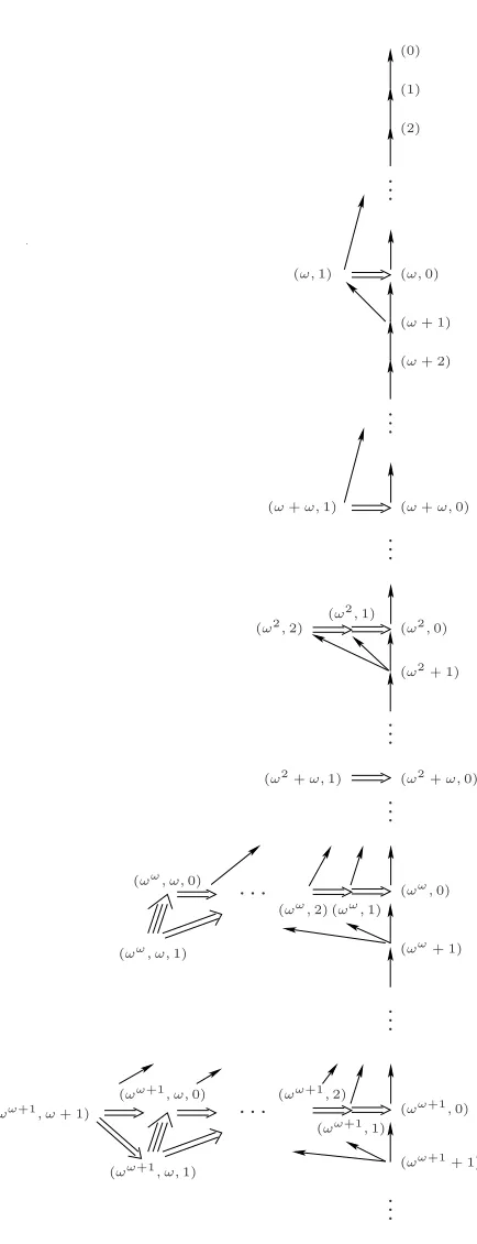
For a visualization of the very top part ofU, namelyUωω+1, see Figure 4.17 Single arrows representR0, double arrows represent R1, and triple arrows represent
R2. While eachRn is transitive, we leave out many of the arrows that should be there as a consequence.
The 1-sheets on this structure are easily identifiable. They are simply those clusters of points that areR1-related to one another. E.g. (ω,1) and (ω,0) form a 1-sheet. U is also clearly a h.l. stratified frame. Indeed,U is a model ofGLP0, andGLP0 is complete with respect toU, as Ignatiev was the first to show. As our proof of this fact makes use of blow-up models, it differs significantly from those in [Ignatiev, 1993] and [Beklemishev et al., 2005], which are both based on syntactic arguments.
Proposition 2.3.6. GLP0⊢φif and only if, for allα~ ∈ U,U, ~α²φ. We first prove soundness, then completeness.
Lemma 2.3.7. GLP0 is sound w.r.t. U.
Proof. We reason by induction on proofs in GLP0, treating only axioms (iii), (iv), and (v). To see Axiom (iv), it is sufficient to note that each relationRn+1 satisfies the condition:
∀α, ~~ β∈U(~αRn+1β~⇒ ∀~γ(~αRn~γ⇔βR~ n~γ))
This is obvious by the definition ofRn+1.
An easy proof that L¨ob’s Axiom is valid relies on the fact that each relation
Rn is transitive and converse-well-founded. It is converse-well-founded simply because all ordinals are well-founded under the <-relation. So given a point
~
α∈ U,αn can decrease only finitely often.18
Finally, while it is possible to prove the validity of Axiom (v), the “Mono-tonicity Axiom”, in a number of ways, we refer the reader to Corollary 3.2.14 below, where we prove that the validity of closed formulas does not change when we augment relations so that ~αRn+1β~ impliesαR~ nβ~ for alln. This is clearly
sufficient for Axiom (v) to hold. ⊣
Our method of showing completeness is to reduce the completeness forU to that for blow-ups of h.l. stratified frames. So we must first prove a number of auxiliary lemmas.
Lemma 2.3.8. For allα, β < ǫ0,Uα+Uβ∼=Uα+1+β.
17This diagram is due to Joost Joosten, having originally appeared in [Joosten, 2004]. 18This fact, however, is not formalizable inPA. In [Beklemishev et al., 2005], a proof of the
..
.
..
.
..
.
..
.
..
.
..
.
..
.
· · ·
(0)
(1)
(2)
(ω,0)
(ω+ 1)
(ω+ 2)
(ω+ω,0)
(ω2,0)
(ω2+ 1)
(ω2+ω,0)
(ωω+ 1)
(ωω+1,0)
(ωω+1+ 1)
(ω,1)
(ωω,0) (ω2,2) (ω
2
,1)
(ω+ω,1)
(ω2+ω,1)
(ωω,1)
(ωω,2)
· · ·
(ωω, ω,0)
(ωω+1,1)
(ωω+1,2)
(ωω+1, ω,0)
(ωω+1, ω+ 1)
[image:22.595.207.424.104.669.2](ωω+1, ω,1) (ωω, ω,1)
Proof. Transfinite induction on β. For the basic case,Uα+U0is isomorphic to
Uα+1 by definition.
Supposeβ=γ+ 1. The induction hypothesis (×2) gives the result:
Uα+Uγ+1 ∼= Uα+
[
δ<γ+1
Uδ+Ue(γ+1)
∼
= Uα+Uγ+U0
∼
= Uα+1+γ+U0
∼
= Uα+1+γ+1
Whenβ=λis a limit, we have the following:
Uα+Uλ ∼= Uα+
[
γ<λ
Uγ+Ue(λ)+
∼
= [
γ<λ
(Uα+Uγ) +Ue(λ)+
∼
= [
γ<λ
Uα+1+γ+Ue(λ)+
∼
= [
γ<α+1+λ
Uγ+Ue(λ)+
∼
= [
γ<α+1+λ
Uγ+Ue(α+1+λ)+
∼
= Uα+1+λ
The penultimate step follows because the efunction only depends on the last
summand of the Cantor Normal Form. ⊣
Lemma 2.3.9. For allα,(U+
α)(ω)∼=Uωα.
Proof. This is shown by transfinite induction on α. First of all, notice we have the following by the definition of sheet-wise blow-up:
(U+ α)(ω):=
[
b
αR0~β
X
i<ω (U~+
β)
(ω)+U+ α
Otherwise put,
(U+ α)(ω)=
[
β<α
X
i<ω (U+
β)
(ω)+U+ α
By the inductive hypothesis,
[
β<α
X
i<ω (U+
β)
(ω)∼= [ β<α
X
i<ω
Uωβ
We claim that, [
β<α
X
i<ω
Uωβ =
[
β<ωα
There are two cases to check: eitherαis a limit or a successor ordinal. Supposeαis a successor ordinal. In particular, suppose α=γ+ 1:
[
β<α
X
i<ω
Uωβ =
X
i<ω
Uωγ
= [
β<ωγ·ω
Uβ
= [
β<ωα
Uβ
On the other hand, ifαis a limit ordinal:
[
β<α
X
i<ω
Uωβ =
[
β<α
Uωβ+1
= [
β<α
Uωβ
= [
β<ωα
Uβ
Finally, putting all of this together,
(U+
α)(ω) ∼=
[
β<ωα
Uβ+Uα+
But this is exactly the definition ofUωα. ⊣
Lemma 2.3.10. Suppose Ais a h.l. stratified model and αis an n-sheet with
Rm empty for allm > n. Then there is someβ such thatBω(α) =Uβ. Proof. Any such n-sheet can be written as U+...++
k , where k is the length of the single n-chain inαand there aren‘+’ symbols. This is simply an n-sheet isomorphic to the very top part of the Ignatiev frame. For simplicity denote it
Uk+n. By the definition of global blowup, we have:
Bω(α) ∼= Bω(U+n
k )
∼
= (Bω(U+n−1
k ) +)(ω) ..
. (n−1 applications of Definition 2.2.28)
∼
= ((...(Bω(Uk)+)(ω)...)+)(ω)
..
. (n−1 applications of Lemma 2.3.9)
∼
= Uβ
Thisβ is therefore determined as in Lemma 2.3.9. ⊣
Seeing asBω(U1)∼=Uωis obvious, the argument in Lemma 2.3.10 gives rise
Corollary 2.3.11. For alln,Bω(U1+n)∼=Uω
n.
This next theorem shows thatU is in a strong sense universal for the class of finite h.l. stratified frames.
Theorem 2.3.12. For any finite h.l. stratified frameA, there is aβ such that
Bω(A)∼=Uβ.
Proof. We show this by induction on rank.19 The case of rank 0 is exactly Lemma 2.3.10. So, consider any h.l. stratified frame A with positive rank. Every such frame can be written as the 0-linear ordering of 1-sheets:
α0R0α1R0...R0αn
The blowup,Bω(A), can be written similarly as the 0-linearly ordered sum of
blow-ups of 1-sheets:
Bω(α0) +Bω(α1) +...+Bω(αn)
By induction hypothesis, each suchBω(αi) is isomorphic to someUβ
i. So:
Bω(A) ∼= Uβ
0+Uβ1+...+Uβn
∼
= Uβ0+1+β1+1+...+βn
The last step is by Lemma 2.3.8. ⊣
Theorem 2.3.13. GLP0 is complete with respect to U.
Proof. If GLP0 0φ, thenJ 0M+(φ)→φ, and by Corollary 2.2.15 there is a h.l. stratified frameAsuch thatA2M+(φ)→φ. Correspondingly,Bω(A)2φ. Theorem 2.3.12 ensures thatBω(A) is isomorphic to some generated subframe
ofU. Therefore,U 2φ. ⊣
In fact Theorem 2.3.13 can be improved to a special subset of points inU. We only mention the result here, and defer the proof to the next section, after further study ofU.
Definition 2.3.14 (Main Axis). ~α ∈ U is a root point if and only if ∀i,
αi+1=e(αi). Themain axis ofU, denotedM, is the set of all root points. We shall writeαb for the root point “generated by” a given ordinalα:
b
α:= (α, e(α), e(e(α)), ...)
Proposition 2.3.15 ([Ignatiev, 1993]). If GLP0 0 φ, then there is a root pointαbon the main axisM, such thatU,αb2φ.
19We have not needed to use the notion ofrank ([Beklemishev, 2007a]) up to this point,
but it is a sufficiently natural notion. Essentially, it is just the maximal depth of nestings of sheets. The formal definition is as follows: For anm-sheetA, if allRn are empty, then
2.4
Words and Ordinals
Our study ofU will center around a class of formulas calledwords, introduced in [Beklemishev, 2004a].20 An important fact, analogous to the Normal Form Theorem forGL,21is that all closed formulas areGLP0-equivalent to a boolean combination of words. Syntactic proofs of this fact were given by Ignatiev and Beklemishev ([Beklemishev, 2004a],[Beklemishev, 2004b],[Ignatiev, 1992]). As a result of Theorem 2.3.13, knowing thatGLP0 is sound and complete for U, we automatically gain a normal form result forU:
Theorem 2.4.1 (Normal Form Theorem). Every closed formula is equiva-lent inU to a boolean combination of words.
We shall use words to study the subsets ofU that correspond to the validity set of a closed formula. We call such setsclosed formula definable subsets, or simplydefinable subsets, ofU. The notationSφ denotes the set of points where
φis true. As a result of Theorem 2.4.1, words will provide a very useful tool in studying such subsets.
By a word we mean a modal formula of the formhnmi...hnoi⊤. Instead of writing out words in this way we shall abbreviate, letting any sequence of nu-merals denote a word. In particular, the empty sequence Λ corresponds to⊤. This will allow us to perform various operations on sequences such as concate-nation: e.g. if 12 denotes h1ih2i⊤ and 01 denotes h0ih1i⊤, then 1201 denotes
h1ih2ih0ih1i⊤. We shall letn, m, ...serve as variables for individual diamonds, and A, B... serve as variables for sequences of diamonds. We will also write, e.g. U, ~β ²A, even though, strictly speaking, this is an abuse of the notation. Finally, letS denote the set of all words, and Sn denote the set of words with only modalitieshmiform≥n.
In order to investigate validity of words, and closed formulas in general, in
U, we introduce the following ordering on U.
Definition 2.4.2. The relation¹defines a rooted partial order on points inU
so that, for any two points~αandβ~,
~
β¹~α⇔(∀i, βi≤αi)
Lemma 2.4.3. For any word A, if U, ~α ² A, then for all β~ ∈ U such that
~
βº~α, we have U, ~β ²A.
Proof. By induction on the length of words. If A= Λ, this is obvious. Suppose this holds for formulas of lengthm, andα~ ²nA, forA of length≤m. Suppose in particular thatαR~ n~δ for some~δ²A. Now take anyβ~ ∈ U such thatβ~ ºα~. We seeβR~ n~γ, where~γ is such that∀i < n γi=βi, and∀i≥n γi=δi. Then we have that~γº~δ, so by the induction hypothesis~γ²A, and henceβ~ ²nA. ⊣
Next, we define a surjective function o from words to ordinals, originally used by Beklemishev to establish a one-to-one ordinal notation system forǫ0 (See Section 1.2).22 The function o is defined by recursion on the width of a word, denotedw(A), wherew(A) is the number of different numerals occurring inA, with a subsidiary recursion on min(A), where min(A) = min(nm, ..., n1) if
A=nm...n1. We writeA− for the result of reducing each element ofAby one.
Definition 2.4.4 ([Beklemishev, 2004a],[Beklemishev, 2005]). The func-tiono:S→ǫ0 is defined:
• IfA= 0k, theno(A) =k
• Otherwise, if A = A10...0Ak, with eachAi ∈ S1 and not all Ai empty, theno(A) =ωo(A−
k)+...+ωo(A−1).
To see that this is a well defined function, note thatw(A−i )< w(A) whenever
k >1. And whenk= 1, min(A−i ) = min(Ai)−1<min(A).
We shall prove that o gives us a means of specifying at what points inU a given closed formula is validated. First, an auxiliary lemma:23
Lemma 2.4.5. If A ∈ S1, then for any word B, we have U, ~β ² A0B if and only ifU, ~β²AandU, ~β²0B.
Proof. For the left-to-right direction, if β~ ²A0B, certainly β~ ² A. Moreover, there is some sequence
~
βRi~γ...Rj~δR0α~
such that eachi, j... > 0 andα~ ²B. Since thereforeα0 < β0, we haveβR~ 0α~, and thusβ~²0B.
For the other direction, ifβ~²A, we have a sequence witnessing this fact:
~
βRi~γ...Rj~δ
AsA ∈S1, eachi, j, .. >0. Therefore, δ0 =β0. Sinceβ~ ²0B, it is also clear that~δ²0B. This meansβ~²A0B. ⊣
Definition 2.4.6. Letι(A) :=o[(A), so thatι(A) is inM.
Proposition 2.4.7. For all words A∈S and pointsβ~ ∈ U,
U, ~β²A⇐⇒β~ ºι(A)
Proof. Induction on the length of A. When A is the empty sequence, this is clear, asι(Λ) = (0).
SupposingAis not empty, we now induct on min(A).
22Ignatiev has also defined such a surjection ([Ignatiev, 1993]), however that in
[Beklemishev, 2004a] is simpler.
If min(A) = 0, thenAcan be written in the formA00A′, withA
0∈S1. Let
ι(A′) =αb
Then by induction hypothesis, β~ ² A′ if and only if β~ º αb. As A
0 ∈ S1, we haveo(A0) =ωγ, where γ=o(A−
0). Thus,
ι(A0) = (ωγ, γ, e(γ), e(e(γ)), ...)
And by the induction hypothesis,~β²A0 if and only ifβ~ ºωcγ. Using Lemma 2.4.5, we have
~
β²A00A′ ⇐⇒ (β~²A
0 & β~²0A′) We know exactly whenβ~²A0; To see when β~²0A′, we have:
~
β²0A′ ⇐⇒ ∃β~′(βR~
0β~′ & β~′ ²A′)
⇐⇒ ∃β~′(βR~
0β~′ & β~′ ºαb)
⇐⇒ β0> α0
We can thus conclude,β~ ²A00A′ if and only ifβ~ºωcγ andβ 0> α0. On the other hand,o(A) =o(A′) +ωo(A−
0)=α
0+ωγ. So,
ι(A) = (α0+ωγ, γ, e(γ), e(e(γ)), ...)
Hence,β~ ºι(A) if and only if β~ ºωcγ and β
0 ≥α0+ωγ. It remains to show
β0> α0 is equivalent toβ0≥α0+ωγ.
The right-to-left direction is obvious. For the other direction, if β0 > α0, thenβ0=α0+δforδ >0. Since e(β0) =e(δ), it follows
δ≥ωe(δ)=ωe(β0)≥ωβ1 ≥ωγ
And soβ0≥α0+ωγ, thus concluding the basic case.
Finally suppose min(A)>0. Since 0 does not occur inA,β~²Aif and only ifβ~′ ²A−, whereβ~′ := (β
1, β2, ...) (each coordinate shifted once to the left). By the induction hypothesis (on min(A)), this is equivalent toβ~′ ºι(A−). Let
ι(A−) =αb. Thenι(A) =ωcα. But clearlyβ~ºωcαif and only ifβ~′ºαb. Putting all of this together:
~
β²A ⇐⇒ β~′²A− ⇐⇒ β~′ºαb ⇐⇒ β~ºωcα ⇐⇒ β~ºι(A)
This concludes the inductive step. ⊣
Proposition 2.4.7 is of central importance. One immediate consequence is thatU is optimal in the sense that it does not have any superfluous points:24
24In the proof of Lemma 2.4.8, as elsewhere, we writeαβ
nto mean ann-stack ofα’s with a βas the top exponent, rather than, e.g. (αn)β, which would denote ann-stack ofα’s raised
Lemma 2.4.8. For any distinct points ~αand β~ in U, there is a word A such thatU, ~α²Abut U, ~β2A.
Proof. Without loss of generality, suppose∀i < n, αi=βi, andαn> βn. Let
b
γ:= (ωβn
n , ..., ωβn, βn, e(βn), e(e(βn)), ...) and supposeo(A) =γ=ωβn
n . Then clearlyU, ~α²nA(since~αRn~δfor~δexactly like ~αup to then-th coordinate and like~γ from then-th on). But we cannot haveU, ~β ²nA, because ifβR~ n~δ, for some appropriate~δ, thenδn< βn=γn. ⊣
We are also now in a position to prove Ignatiev’s strengthening of complete-ness, to the effect that it is possible to falsify any non-theorem ofGLP0on the main axis.
Theorem 2.4.9. If GLP00φ, there isαb∈M such that U,αb2φ.
Proof. If GLP0 0 φ, then by Theorem 2.3.13,U 2φ. By Corollary 2.4.1, we can assume φis in conjunctive normal form, where each “atom” is a word or the negation thereof. It follows that U 2 A → (A1∨...∨Aj) for some such conjunct ofφ. I.e, there is some pointα~ such that~α²A, but~α2(A1∨...∨Aj). By Proposition 2.4.7, ~αºι(A), and α~ ²ι(Ai), for each i≤j. Putting these together givesι(A)²ι(Ai), for eachi≤j, so ι(A)2(A1∨...∨Aj). In other words,ι(A)2A→(A1∨...∨Aj), and henceι(A)2φ, as desired. ⊣
3
The Canonical Frame of GLP
0Recall the definition of thecanonical frame:
Definition 3.0.10. Thecanonical frameforGLP0 is defined:
C0:= (W0, R0
n:n < ω)
• W0 is the set of maximal-GLP0-consistent sets.
• xR0
ny if and only if for all closed formulasφ, φ∈y implieshniφ∈x. A very natural question, given completeness and soundness of GLP0 with respect to U, is what the relationship is between U and C0. Certainly every finite GLP0-consistent set is a subset of the formulas true at some point in
U. But we might also wonder whether every maximal GLP0-consistent set is satisfiable at a single point. The answer turns out to be no, as we shall see.
After discussing the relationship between descriptive frames and canonical frames, we will be able to show thatU is not the canonical frame of GLP0. The rest of the section will be dedicated to turningU into a descriptive frame
3.1
Descriptive General Frames
3.1.1 Basic Facts
Definition 3.1.1 (General Frames). Ageneral frame25 in the basic modal language is a pair (F, A) such that F= (F, R) and A⊆ P(F), which is closed under finite union, finite intersection, complement, andR−1.
In other words, a general frame is simply a frame along with a distinguished set of subsets, which also defines an algebra over the frame. For the extension to the polymodal case, we must simply add closure underR−1
n for eachn.
Remark 3.1.2. Though we will not be concerned with valuations in this sec-tion, as we are only dealing with the closed fragment, it is worth mentioning that a so calledadmissible valuation on a general frame, giving rise to amodel based on a general frame, is one whose values are restricted to sets inA. For any logicL, if we consider the canonical frameCLand letCbe the set of sets of the form{Γ :φ∈Γ,Γ is maximal-L-consistent}, withφranging over all formulas, it is easily seen that (CL, C) is a general frame. From this it follows that any logic is sound and complete with respect to some class of general frames.26 This of course means that we do have a very abstract completeness result for full
GLP. However, a challenge would be to describe what such a class looks like in some detail, analogous to our treatment ofC0in the coming pages.
The algebraic flavor of general frames is by no means merely superficial. Given a general frameG= (F, A), we can form amodal algebra G∗, taking A as the underlying set andR−1 as an operator. A formulaφ will be valid inG just in case the identityφ=⊤is a valid identity ofG∗, so Gand G∗ are in a sense modally equivalent.
In the other direction, it is also always possible to form a general frame from a modal algebra. From a modal algebraAwe obtain the so calledgeneral
ultrafilter frame A∗, the underlying set being the set of ultrafilters ofA, with
relations and the setAdefined appropriately. As before, for a formulaφ,φ=⊤
is an identity ofAif and only if φis valid inA∗.
This explanation is of course far from comprehensive, but the details of this correspondence are not crucial. An important fact about these operations is that the following isomorphism always holds, whereAis any modal algebra:
(A∗)∗∼=A
That is, if we form the general ultrafilter frame and then take the associated algebra of this general frame, we will always end up with something isomorphic toA. The converse, however, does not hold for arbitrary general frames:
(G∗)∗∼=G
25The definitions and background results in this section are drawn from a combination of
[Blackburn et al., 2001] and [Chagrov and Zakharyaschev, 1997].