Iterated Majority Voting
St´ephane Airiau and Ulle Endriss
Institute for Logic, Language and Computation University of Amsterdam
{s.airiau,u.endriss}@uva.nl
Abstract. We study a model in which a group of agents make a
se-quence of collective decisions on whether to remain in the current state of the system or switch to an alternative state, as proposed by one of them. Examples for instantiations of this model include the step-wise refinement of a bill of law by means of amendments to be voted on, as well as resource allocation problems, where agents successively alter the current allocation by means of a sequence of deals. We specifically focus on cases where the majority rule is used to make each of the collective decisions, as well as variations of the majority rule where different quo-tas need to be met to get a proposal accepted. In addition, we allow for cases in which the same proposal may be made more than once. As this can lead to infinite sequences, we investigate the effects of introduc-ing a deadline boundintroduc-ing the number of proposals that can be made. We use both analytical and experimental means to characterise situations in which we can expect to see a convergence effect, in the sense that the expected payoff of each agent will become independent from the initial state of the system, as long as the deadline is chosen large enough.
1
Introduction
We consider the very general problem where a finite set ofagents must choose one alternative among many, and we are interested in decentralised solutions. The alternatives may represent different policies, world states, or allocations of resources, etc. One simple idea is to start with an initial current alternative, let a random agent propose a different alternative, and organize a vote between these two alternatives. The processiterates using the winner of the election as current alternative. Unfortunately, with no restriction on the agents’ preferences, this simple process may iterate forever. In this paper, we investigate the possibility of using a bound on the number of iterations. In particular, we investigate the problem of determining whether the choice of the bound can guarantee that no agent benefits unduly from the choice of the initial alternative.
In this case, every possible allocation of resources constitutes an alternative and proposing a new alternative means proposing a deal regarding the reallocation of some items. Here, the voting rule used would typically require each agent affected by the proposal to give their consent. Finally, recent work in computa-tional social choice has shown that decomposing combinatorial voting problems into a sequence of smaller elections has a number of advantages [3].
In general, there are many possible choices of a voting rule. In this paper, we focus on the majority rule, which specifies that a proposal is accepted if at least half of the concerned agents (those that are not indifferent) vote in favour. This is clearly a very natural choice, and it is the only rule that is anonymous, neutral, and monotone (May’s Theorem [4]). We also consider generalisations of the majority rule, where a quota different from 50% may be needed to accept a proposal. For example, for some important elections, a higher proportion of votes in favour of an alternative is needed, e.g., a two-thirds majority in parliament is needed to change the constitution. As we allow agents to make the same proposal over and over, there is the possibility for cycles. This phenomenon is linked to the fact that the preference relation we obtain when several individual preferences are aggregated by means of the majority rule need not be transitive. In social choice theory, one approach to address this problem has been to restrict the range of allowed preferences, e.g., to single-peaked preferences or preferences meeting Sen’s triple-wise value restriction [5]. When we have no control over the agents’ preferences, we need to modify the protocol to induce the agents to choose a good social alternative. A simple solution to the problem of cycles is to introduce a deadline that limits the number of iterations.
We assume that the agents’ preferences are common knowledge and that agents are strategic: they will make proposals and vote in elections so as to max-imise their expected payoff. What would be a good choice of deadline under these circumstances? If it is small, the choice of initial state will play an important role for the final outcome. If it is large, as we shall see, it is sometimes the case that the expected payoff of an agent becomes independent of the initial state, which provides some level of fairness. Our aim in this paper is to get a clearer understanding of such convergence effects.
The remainder of this paper is as follows. Section 2 further motivates and defines our model. In particular, we detail how strategic agents can compute their best moves using backward induction. Section 3 formally defines the notion of convergence as used here and establishes sufficient conditions on a game for being convergent. Then, Section 4 takes this analysis further by mapping out the convergence behaviour for a wider class of games by means of an experimental study. We conclude with a discussion about related work and present future axes of research.
2
The Model
We study games consisting of a finite setN ofnagents and a finite setX ofm
is assumed to be common knowledge. Each agent is rational, i.e., it maximizes its expected utility. The utility functions are represented together as anm×n
matrixU0, withU0(x, i) =ui(x). We do not assume that utility is transferable:
the utility of two agents may not be comparable (e.g., agents can use different currencies). However, we do assume that agents will use their knowledge of the utility of other agents for predicting their behaviour.
A game proceeds in successive iterations. At each iterationt, there is a cur-rent alternativex(t) (a given allocation, a current bill). One agent is randomly selected, with equal probability, to propose a new alternativex⋆
to be considered (e.g., a new allocation, an amendment to the current bill). An agent may pro-pose an alternative that was already propro-posed in the past; and it may propro-pose to maintain thestatus quoby proposingx⋆
=x(t). The agents vote betweenx⋆
and x(t). If the proposed alternative wins the election, and we will present the criterion to win an election next, it replaces the current alternative for the next iteration. Else, the current alternative remains in place for the next iteration.
Elections are decided using aquota systemfor some fixed quotaq: a proposal will be declared the winner iff it receives at least q percent of the votes. More precisely, ifn⊕agents are voting in favour andn⊖against a proposal (and some agents may abstain), then the proposal is accepted if n⊕ > q·(n⊕+n⊖). The standard majority rule is the quota system withq = 50%. When the majority rule is used, cycles may occur. The same is true for quota systems with q 6= 50%. In the presence of a cycle, the sequence of elections could be infinite. In order to force the eventual choice of an alternative, we propose the use of a deadline limiting the number of iterations to be played. The following definition summarises the components that make up a game:
Definition 1 (Game). A game is a quadruple hN, X, U0, qi, where N with
n = |N| is a finite set of agents, X with m = |X| is a finite set of states (or alternatives), U0 is an m×nmatrix defining the utility each agent assigns
to each state, andq∈[0,1]is a quota (typically expressed in percent).
Playing a game requires us to also specify adeadline, i.e., the number of iterations to be played, and aninitial statefrom X.
2.1 Backward induction
Agents are assumed to be expected-utility maximisers, i.e., the goal of a proposal or a vote is to maximise expected utility in the final state. We now discuss how to perform this strategic vote and strategic choice of proposals.
Let the matrixWt of sizem×mspecify the transition between the alterna-tives at iterationt. An entryWt(x, y) ofWtis the probability to have alternative
y become the current alternative at the next iteration when alternative xwas current at iterationt. A row ofWtis a probability distribution over the
i.e.,Ut(x, i) is the expected payoff of agentifor alternativexat iterationt. We haveUt+1=Wt+1·Ut, and therefore:
Ut+1= 1
Y
τ=t+1
Wτ
!
·U0=Wt+1·Wt·Wt−1·. . .·W1·U0
Next, we discuss how to computeWt+1 from Ut. Let us assume that the agents
know what to propose and how to vote during thetth
iteration for any alternative
x∈X. Because of the common knowledge assumption on the utility functions, the possible proposals and votes of any agents are also known, hence the matrices
Wt,Wt−1, . . .,W1 are known. What should an agent do during iterationt+ 1?
How to vote?The decision depends on the comparison of the expected utility of the current alternativex(t) with the one of the proposed alternativex⋆
, i.e., agent i will vote in favour of the proposal when Ut(x⋆, i) > Ut(x(t), i) and
against whenUt(x⋆
, i)< Ut(x(t), i). Note that the agent does not vote in case it is indifferent between the two alternatives.
What to propose? First, the agent needs to compute the outcome of the vote between the current statex(t) and each possible alternativex′∈X. LetXw
⊆X
denote the set of winning alternatives againstx(t). For agent i, the set of best proposals isPi = argmaxx′∈XwUt(x
′, i). If the expected utility of the alternatives inPi is greater thanUt(x(t), i) (the expected utility of the current alternative), then agent i proposes with equi-probability one of the alternatives inPi. Else, agent i is content with the current alternative and proposes maintaining the status quo (there is no decision to make since x⋆
= x(t)). Since each agent has an equal probability to be selected to make a proposal, we can compute the probability of any alternative to be proposed. And since any alternative that is proposed is winning against the current alternative, we can compute the probability of an alternative to become current at the next iteration.
To summarise, a gamehN, X, U0, qiinduces a sequence ofm×mtransition
matricesW1, W2, . . ., as described above, as well as a sequence ofm×nmatrices
U1, U2, . . ., fixing the expected payoffs for each agent at each iteration, with
Ut+1=Wt+1·Ut. Here, “iteration 1” is the final iteration/step in a play of the
game, “iteration 2” is the penultimate iteration, and so forth. These matrices allow us to study the game for all possible choices of initial current alternative.
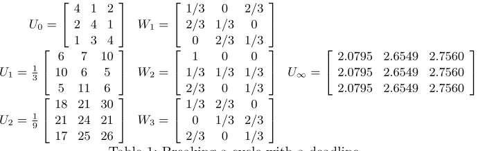
2.2 Example: a cycle with majority voting
Consider the following problem with 3 agents and 3 states. The utility vectors are: h4,1,2ifor state a, h2,4,1i for state b and h1,3,4ifor state c. The corre-sponding matrixU0is shown in Table 1. With no deadline, the agents would be
U0=
2
4 4 1 2 2 4 1 1 3 4
3
5 W1=
2
4
1/3 0 2/3 2/3 1/3 0
0 2/3 1/3 3
5
U1= 1 3
2
4
6 7 10 10 6 5
5 11 6 3
5 W2=
2
4
1 0 0
1/3 1/3 1/3 2/3 0 1/3
3
5 U∞= 2
4
2.0795 2.6549 2.7560 2.0795 2.6549 2.7560 2.0795 2.6549 2.7560
3
5
U2= 1 9
2
4
18 21 30 21 24 21 17 25 26
3
5 W3=
2
4
1/3 2/3 0 0 1/3 2/3 2/3 0 1/3
3
[image:5.612.139.484.115.224.2]5
Table 1: Breaking a cycle with a deadline
State awould lose an election against state c, and win an election against state b. If the current alternative is state a one step before the deadline, the second and third agents should propose statec, the first agent should propose the status quo. As the agents are chosen to make a proposal with equi-probability, the probability to stay in a is 1
3, the probability to move to c is 2
3, and the
probability to move tob is zero. This provides the first row of the matrix W1
in Table 1. We carry this reasoning to completeW1. The expected utility of the
agents one step before the deadline is U1 =W1U0. We iterate the reasoning to
obtain the matricesW2,U2, etc. We note that, in this example,W1,W2 andW3
are different. We have implemented the iterative algorithm for computing the matricesWtandUt. For large values oft,Utconverges to a particular matrix (see U∞ in Table 1). That is, fort large enough, the expected utility of each agent is independent of the initial state (e.g., agent 1’s expected utility approaches 2.0795). Hence, if the deadline is far enough, no agent can take advantage of the initial choice of alternative. Finally, note that, in the limit, the expected utility of an agent is not simply the average utility over the 3 alternatives.
3
Convergence
The example given in the previous section shows that there are instances of games where we will observe some kind of convergence. For the example in question, we have seen that the expected payoff of any given agent for any given initial state will converge to a certain value as we increase the deadline (we call thisintra-state convergence). We have also observed that the expected payoff will become less and less dependent on the initial state as we increase the deadline (we call thisinter-state convergence). In this section, we will define these notions of convergence formally and identify some classes of games for which convergence can be guaranteed.
3.1 Types of convergence
Definition 2 (Intra-state convergence). A game hN, X, U0, qi is said to
be intra-state convergent if, for any agent i ∈ N and any state x ∈ X, limt→∞[Ut(x, i)−Ut+1(x, i)] = 0.
Next, we define a game as being inter-state convergent if, for any agent and any two states, the difference in expected payoff for making either one of these states the initial state can be made arbitrarily small when we increase the deadline:
Definition 3 (Inter-state convergence). A game hN, X, U0, qi is said to be
inter-state convergent if, for any agent i ∈ N and any two states x, x′ ∈ X, limt→∞[Ut(x, i)−Ut(x′, i)] = 0.
Inter-state convergence provides a level offairness: as long as we choose a suffi-ciently large deadline, the choice of initial state will not affect the expected payoff of the individual agents. This does not mean that all agents can be expected to do equally well, but it does mean that one important parameter that determines how a game is played (the initial state) does not influence the (expected) out-come. Intra-state convergence does not directly affect fairness, but offers some level ofrobustnessof the mechanism: expected payoffs will not depend on the ex-act deadline chosen (for instance, we would avoid situations whereby an agent’s expected payoff could depend on whether the chosen deadline is odd or even).
Our example did exhibit both types of convergence. Both are entailed by a third notion of convergence, expressed in terms of the transition matrices Wt
induced by a game.
Definition 4 (Fundamental convergence). A game hN, X, U0, qiis said to
be fundamentally convergent if the limit of the product of its transition matrices
W = lim
t→∞
1
Y
τ=t
Wτ is a matrix in which all row vectors are identical.
Definition 4 is reminiscent of the Fundamental Limit Theorem for regular Markov chains, which says that ifP is the transition matrix of a regular Markov chain, then limn→∞P
n
=W for some matrixW with identical row vectors [6]. Recall that a stochastic matrix P is a matrix defining a regular Markov chain if there exists a ksuch thatPk
has only non-zero elements. In particular, the theorem applies whenPitself only has non-zero elements. Inspection of the standard proof of the Fundamental Limit Theorem shows that the same is true for the product of severaldifferent matrices, provided that an infinite number of them are zero-free. While there are similarities to our scenario, we stress that the Fundamental Limit Theorem doesnot apply here, because the transition matrices generated by our games need neither be zero-free nor regular.
Before linking the three definitions of convergence, we state a simple property of stochastic matrices. The proof is standard and omitted for lack of space.
Lemma 1. LetAandB bem×mstochastic matrices. IfB has all row vectors
identical, then A·B=B.
Proposition 1. If a game is fundamentally convergent, then it is also
Proof. LetW = limt→∞Q
1
τ=tWτfor the game under consideration. Suppose the
game is fundamentally convergent, i.e.,W is a matrix of identical row vectors. Then the game is also inter-state convergent: if we multiply W with the payoffs for agenti, then we get the same expected payoff for any initial state.
Next, we show that intra-convergence also follows. By Lemma 1, asQ1
τ=tWτ
converges to a matrix with identical rows, Wt+1·Q 1
τ=tWτ converges to that
very same matrix. The former determines Ut(x, i), while the latter determines
Ut+1(x, i). Hence, their difference must converge to 0. ⊓⊔
Furthermore, it is not hard to verify that inter-state convergence implies intra-state convergence. Intra-intra-state convergence is weaker than the other two forms of convergence. There are games that are intra-state convergent but not inter-state convergent. A simple example would be a game with 2 agents, 2 states, and
q= 50%, where agent 1 prefers stateaand agent 2 prefers state b. Then, if the initial state isa, this will remain the status quo, independently of the deadline (and analogously for the case wherebis the initial state). The transition matrices for this game are all equal to the identity matrix. Hence, inter-state convergence is not satisfied (your expected payoff is equal to the utility you assign to the initial state), while intra-state convergence is (your expected payoff remains constant when we vary the deadline).
3.2 Sufficient conditions
We will now identify sufficient conditions for a game to be convergent. There are some clear-cut cases, when the quotaq takes extreme values. First, ifq = 0%, i.e., when a single agent in favour is sufficient for a proposal to be accepted, then all forms of convergence are satisfied. In such a game, whichever agent is chosen to make a proposal in the last iteration will propose their favourite state, and that motion will carry—independently from the current state. Hence, W1
(the transition matrix for the last iteration) will be a matrix with all rows equal. Therefore, by Lemma 1, also the product W of all transition matrices will be such a matrix, which means that the game will satisfy the convergence condition of Definition 4, and by Proposition 1 also all other notions of convergence.
Second, ifq= 100%−ǫ, i.e., when only proposals opposed by no agent are accepted, then a proposal is accepted iff it represents a Pareto improvement. Hence, the final state will be Pareto optimal—provided the deadline is chosen large enough. But if there is more than one Pareto optimal state, then the expected payoff can be different for an agent if either one of these Pareto optimal states is selected as the initial state. Therefore, inter-state convergence is not generally satisfied (and neither is fundamental convergence). Only in very special cases, such as when all agents are indifferent between all states, would be obtain inter-state convergence.
U0=
2
6 6 4
4 4 4 6 2 3 2 6 2 3 0 6
3
7 7 5
W1=
2
6 6 4
1 0 0 0
2/3 1/3 0 0 0 1/3 1/3 1/3 1/3 1/3 0 1/3
3
7 7 5
U∞= 2
6 6 4
4.3676 3.0288 3.9973 4.3676 3.0288 3.9973 4.3676 3.0288 3.9973 4.3676 3.0288 3.9973
3
[image:8.612.143.478.116.163.2]7 7 5
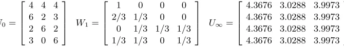
Table 2: Example with a unique Condorcet winner: the final outcome may not be the Condorcet winner.
h4,4,4i), but the expected payoffs in the limit are not the payoffs of the Con-dorcet winner. This is because from the state with payoffh2,6,2i, no agent has an incentive to propose the Condorcet winner.
We now analyse the case of games with two states in detail.
Proposition 2. Any game with two states is intra-state convergent.
Proof. In games hN, X, U0, qi with |X| = 2, each transition matrix is of the
following form:
Wt =
p 1−p
1−q q
Two special cases arep=q= 1 (the identity matrix) andp=q= 0 (the “switch matrix”). We first claim that no transition matrix can be such a switch matrix: if all agents are indifferent between both states in iteration t, then Wt is the identity matrix. Otherwise, w.l.o.g., assume agent 1 prefers state 1 in iterationt. Then agent 1 will propose thestatus quo when in state 1, sop≥ 1
n. This proves
our claim.
So each transition matrix will either be the identity matrix or different from both the identity matrix and the switch matrix. We now distinguish two cases:
(i) There exists a transition matrix Wt that is the identity matrix. Then Ut+1=Ut, andWt+1and all subsequent transition matrices are also the identity
matrix. Hence, from point ton the expected payoff for any given state will not change anymore and we have intra-state convergence as required.
(ii) There does not exist a transition matrix that is the identity matrix. We shall prove inter-state convergence in this case (which entails intra-state convergence). W.l.o.g. we analyse the expected payoff of agent 1. Suppose xis its expected payoff for state 1 andyfor state 2, at some step of the process. The expected payoffs for the next step are computed as follows:
p 1−p
1−q q
· x y =
y+p·(x−y)
x+q·(y−x)
Consider the difference|x−y|. In the next step, this difference becomes|(y+p·
(x−y))−(x+q·(y−x))|=|p+q−1| · |x−y|. The factor of change|p+q−1|is of course≤1. But we can give a better bound. We know that neitherp=q= 0 norp=q= 1. We also know that pand qmust be multiples of 1
n, wheren is
the number of agents. (This follows from the rules of the game: each of the n
propose thestatus quoor the other state with certainty—for the special case of two states no agent will ever randomise between several top proposals). Hence,
|p+q−1| ≤1− 1
n. Now, ifxand y are the actual utilities for the two states, t steps before the deadline the difference in expected payoffs can be at most (1− 1
n) t
· |x−y|. Therefore, as t goes to infinity, this difference must go to 0. This is the case for both agents, meaning that inter-state convergence holds as
claimed. ⊓⊔
Proposition 3. Any game with two states and a quota ofq <50%is inter-state
convergent.
Proof. The proof of Proposition 2 shows that, first, no transition matrix can be the “switch matrix”; and second,if no transition matrix is the identity matrix (or the switch matrix), then inter-state convergence is satisfied. The only remaining possibility is when there exists a iterationtsuch thatWtis the identity matrix. We distinguish two cases:
(i) First, assume all agents are indifferent between states 1 and 2 in iterationt. Then we clearly have convergence.
(ii) Otherwise, w.l.o.g., assume agent 1 strictly prefers state 1 in iterationt. Then the only explanation for agent 1 not proposing state 1 when in state 2 is that such a proposal would not make the quota. Hence, asq <50% by assump-tion, at least 50% (1−q) of the concerned agents (those not indifferent between state 1 and state 2 in iterationt) must prefer state 2. But then, when in state 1, each of these agents would propose to move to state 2 and any such proposal would get accepted, so the probability of moving from state 1 to 2 in iterationt
must be >0. Hence,Wt cannot be the identity, and we have a contradiction.⊓⊔
The bound on the quota in Proposition 3 is tight: the example sketched after Proposition 1 demonstrates that inter-state convergence cannot be guaranteed anymore for quotas q ≥ 50%. In the next section, we will analyse our games experimentally, to see to what extent the trends reflected by Propositions 2 and 3 extend to larger games.
4
Experimental analysis
The aim of the experiments is to investigate what parameters affect convergence. In all the experiments we performed, we have always observed intra-state conver-gence. In the following, we will therefore only report on inter-state convergence (and hence, we write simply “convergence” to denote inter-state convergence).
4.1 Varying the utility range
of integers{0,1, . . . , umax}. Here we focus on uniform distributions (other cases are also interesting and left for future work). The goal of our the first experiment is to answer the question: how does the set of possible utility values affect the rate of convergence?
When a continuous uniform distribution is used to generate the utility values, the preference order on the set of alternatives is strict with probability one. When a discrete distribution is used, however, the agent may have a weak preference order as some alternatives may receive the same values. For a fixed number of alternatives, the smallerumax, the more likely the agents have a weak order. In the extreme case ofumax= 1, agents have dichotomous preferences (i.e., either they approve or disapprove the alternative).
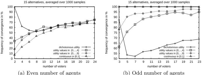
We fixed the number of states to 15 and varied the number of agents in
{2. . .24}. We generated 1000 utility matricesU0for each number of agents and
checked for convergence for a quota of 50%. The results are provided in Figure 1.
0 10 20 30 40 50 60 70 80 90 100
2 4 6 8 10 12 14 16 18 20 22 24
frequency of convergence in %
number of voters 15 alternatives, averaged over 1000 samples
dichotomous utility utility values in {0,...,4} utility values in {0,...,9} continuous in [0,1]
(a) Even number of agents
50 55 60 65 70 75 80 85 90 95 100
3 5 7 9 11 13 15 17 19 21 23
frequency of convergence in %
number of voters 15 alternatives, averaged over 1000 samples
dichotomous utility utility values in {0,...,4} utility values in {0,...,9} continuous in [0,1]
[image:10.612.140.486.323.452.2](b) Odd number of agents Fig. 1: Frequency of convergence forq= 50%
First, we do not always observe convergence. Convergence is more frequently observed when the number of agents is large. Then, the frequency of convergence is higher when the number of agents is odd than when it is even. For an even number (Figure 1a), there is no significant difference between the different gen-erators, except for very small numbers of agents.1
For an odd number of agents (Figure 1b), the convergence occurred for all the tested cases with a continuous distribution. Finally, convergence is less frequent whenumaxis small.
These observations suggest that convergence is more frequent when there are fewer ties between alternatives. When ties are extremely unlikely, we observe high frequency of convergence (i.e., when the number of agents is odd and utilities are
1
drawn from a continuous distribution; or when the number of agents is large, as exact ties would be required). When ties are likely, however, we observe a lower frequency of convergence (i.e., when the number of agents is even and small and the utility values are drawn from a continuous distribution; or when utilities are drawn from a discrete distribution and umax is small). Experiments with
different numbers of alternatives did not alter our conclusions.
4.2 Varying the quota
For two-state games, we have seen that inter-state convergence is guaranteed for quotas<50% and can fail for greater quotas. Our second experiment is aimed at checking whether the same trend can be observed for larger games, and at getting an understanding of the likelihood of convergence, when it cannot be guaranteed. We have used 15 alternatives and a population of 100 agents and we have randomly generated 1000 matricesU0. The results are shown in Figure 2.
0 20 40 60 80 100
40 45 50 55 60 65 70 75 80
frequency of convergence in %
quota in %
15 alternatives, 100 agents, averaged over 1000 samples
[image:11.612.204.408.324.468.2]dichotomous utility utility values in {0,...,4} continuous in [0,1]
Fig. 2: Frequency of convergence with different quotas
Forq < 50%, we always observe convergence, which leads us to conjecture that Proposition 3 generalises to games with any number of states. For higher quotas, we do not always observe convergence (about 80% of the time for q= 50%); and for quotas q ≥ 60%, we have never observed convergence in our experiments. Still, even forq= 100%, it is clear that cases satisfying convergence do exist (e.g., if all agents are indifferent between all states); such cases are just very unlikely to occur, certainly for our method of data generation.
5
Conclusion
We have proposed a model for iterated voting, where a group of agents make a social choice by implementing a sequence of binary decisions between thestatus quo and an alternative proposal. Each decision is made using a quota rule.
Our model is related to the study oftournaments [7] as we can think about our generic approach as a walk in the majority graph. The Markov solution is related to our work as it considers a random walk in the majority graph, and an outcome is in the solution set when it has a positive probability of being the current outcome in the limit. Our model differs by allowing strategic behaviour (i) in the choice of the proposed alternative and (ii) in the vote (an agent may vote in favor of a less preferred outcome in the short run if this promises a better outcome in the long run). Models closer to ours have been studied in political science, e.g., by Baron [8], although in that model each voter receives a payoff at every time step, while we only ascribe utility to the final state. In the work by Penn [9] another difference is that the challengers are drawn from a given probability density rather than proposed by the agents.
For the case of games with just two states, we have shown that the expected payoff of each agent converges as the deadline increases, when the initial state is fixed. For games with two states and a quota of less than 50%, we have further-more shown that the expected payoff is independent of the initial state, which offers a level of fairness. Our experimental study shows that this trend generalises also to larger games. For the majority rule, corresponding to a quota of exactly 50%, we have seen that convergence is frequent, but cannot be guaranteed. We have also illustrated how the range of possible utility values an agent may assign to an alternative, and thereby the likelihood of ties, affect convergence.
Future work should be directed towards formulating further conditions under which convergence can be guaranteed, and prediction of a bound guaranteeing that no agent benefits from the choice of the initial state.
References
1. Rosenschein, J.S., Zlotkin, G.: Rules of Encounter. MIT Press (1994)
2. Endriss, U., Maudet, N., Sadri, F., Toni, F.: Negotiating socially optimal allocations of resources. Journal of Artif. Intell. Res.25(2006) 315–348
3. Lang, J., Xia, L.: Sequential composition of voting rules in multi-issue domains. Mathematical Social Sciences57(3) (2009) 304–324
4. May, K.O.: A set of independent necessary and sufficient conditions for simple majority decisions. Econometrica20(1952) 680–684
5. Sen, A.K.: Collective Choice and Social Welfare. Holden-Day (1970)
6. Grinstead, C.M., Snell, J.L.: Introduction to Probability. 2nd edn. American Math-ematical Society (1997)
7. Laslier, J.F.: Tournament Solutions and Majority Voting. Springer (1997)
8. Baron, D.P.: A dynamic theory of collective goods programs. The American Politi-cial Science Review 90(1996) 316–330
9. Penn, E.M.: A model of farsighted voting. American Journal of Political Science