Running head: Prospective memory in the red zone
Accepted, Journal of Experimental Psychology: Applied, 20/02/2019.
Luke Strickland
1,2, David Elliott
2, Michael David Wilson
1, Shayne
Loft
1, Andrew Neal
3, & Andrew Heathcote
21
The School of Psychology,
The University of Western Australia, Australia
2
The School of Medicine,
The University of Tasmania, Australia
3
The School of Psychology,
The University of Queensland, Australia
Address for Correspondence
Luke Strickland,
School of Psychological Science, M304,
The University of Western Australia,
35 Stirling Highway,
6009 Perth, Australia
Email:
[email protected]
Author Note
This research was funded by the Australian Government through the Australian Research
Council (DP160101891). We thank Daniel White for programming the maritime surveillance
Abstract
Remembering to perform a planned action upon encountering a future event requires event-based
Prospective Memory (PM). PM is required in many human factors settings in which operators
must process a great deal of complex, uncertain information from an interface. We study
event-based PM in such an environment. Our task, which previous research has found is very
demanding (Palada et al., 2018), requires monitoring ships as they cross the ocean on a display.
We applied the Prospective Memory Decision Control Model (Strickland, Loft, Remington &
Heathcote, 2018) to understand the cognitive mechanisms that underlie PM performance in such
a demanding environment. We found evidence of capacity sharing between monitoring for PM
items and performing the ongoing surveillance task, whereas studies of PM in simpler paradigms
have not (e.g., Strickland et al., 2018). We also found that participants applied proactive and
reactive control (Braver, 2012) to adapt to the demanding task environment. Our findings
illustrate the value of human factors simulations to study capacity sharing between competing
task processes. They also illustrate the value of cognitive models to illuminate the processes
underlying adaptive behavior in complex environments.
Keywords: prospective memory, linear ballistic accumulator model, unmanned aerial vehicle
Public Significance Statement
We introduce a model that specifies the cognitive processes underlying Prospective Memory
tasks, which require completion of deferred actions at some point in the future, and we apply it to
a laboratory simulation of a complex, dynamic maritime surveillance task. Our model identifies
multiple cognitive mechanisms that underlie performance in complex environments, with several
Often, humans must remember to perform a planned action at some point in the future, a
task referred to as Prospective Memory (PM; Einstein & McDaniel, 1990). In complex
industrial-systems such as air traffic control and maritime surveillance with unmanned aerial
vehicles (UAVs), PM tasks arise frequently, and are commonly reported as a source of human
error (Dismukes, 2012). One common form of PM is event-based PM, in which the operator
must perform a planned action when they encounter a particular environmental cue. For
example, in maritime surveillance, some situations (e.g., military training operations) require the
formation of temporary safety-zones under an operators’ jurisdiction. In these circumstances,
operators must remember to deviate from routine vessel classification, and instead remember that
vessels matching particular features and travelling within the safety-zone must be reclassified
and flagged for further evaluation (Nilsson, Van Laere, Ziemke, & Edlund, 2008).
Although field studies have been critical for identifying PM demands in complex
workplace systems (e.g., Shorrock, 2005; Rothschild et al., 2005; Dismukes, Berman, &
Loukopoulos, 2007), use-inspired laboratory experiments are also critical to understand the
specific psychological mechanisms underlying the phenomena identified by field studies
(Morrow, 2018; Stokes, 2011). For example, simulations of air traffic control have been used to
identify factors that affect PM and to test the effectiveness of work design interventions such as
memory aids (see Loft, 2014 for a review). However, applied PM research such as this has relied
on verbal theorizing about the psychological mechanisms underlying PM. There are many
potential advantages in extending this approach with quantitative “human performance
modeling” (Byrne & Pew, 2009). For example, quantitative modeling can provide a unified
account of disparate performance data, characterize the latent cognitive mechanisms underlying
within systems when human in-the-loop testing is not feasible. Recently, a quantitative model of
event-based PM, “Prospective Memory Decision Control” (PMDC; Strickland, Loft, Remington,
& Heathcote, 2018), was shown to provide a cohesive and informative account of the cognitive
processes underpinning event-based PM in a basic laboratory paradigm.
PMDC may be a suitable basis for human performance modeling of event-based PM in a
wide range of human factors applications. However, real-world cognitive demands can differ
greatly from the demands of simple laboratory tasks. Notably, in previous studies, PMDC
indicated that monitoring for PM items was possible at no cost to the information processing of
concurrent tasks, suggesting that PM was able to rely upon surplus cognitive resources
(Strickland et al., 2018). By contrast, in many settings of interest, such as aviation and defense,
operators must integrate a great volume of complex and transient information from display
interfaces and operate in dynamic and uncertain environments. Under such demands, cognitive
resources may not remain in surplus. Indeed, practitioners are often particularly interested in
identifying the level of cognitive demand that exceeds an operator’s capacity, because further
demands beyond this point may impede the operator’s ability to perform within safety
thresholds. This point is known as the 'red zone' (Wickens, Hollands, Banbury, & Parasuraman,
2015). To date, we do not know if or how PMDC can account for human behavior observed in
the red zone. In the current study, we attempt to apply PMDC to performance in a simulated
maritime surveillance task that is more representative of the type of complex task relevant to
practitioners than the simple paradigm for which PMDC was originally developed. Critically, our
paradigm is capable of raising task demand to the red zone (Palada, Neal, Tay, & Heathcote,
2018), and generalizing PMDC to complex tasks with high cognitive demand, thereby bridging
discussing our study further, we begin by introducing the general paradigm for studying
event-based PM in the laboratory, and relevant previous findings.
Prospective Memory in the Laboratory
PM is typically examined in the laboratory using the Einstein and McDaniel (1990)
paradigm. In this paradigm, participants perform an ongoing task (e.g., lexical decision, deciding
whether strings of letters are words or non-words), and are asked to make an alternative task
response at some point in the future (the PM task). In event-based PM, the PM task is to respond
to items with certain target attributes (e.g., press an alternative key when you see a word
containing the letter string containing ‘tor’). Often, mean RTs to non-PM items are slower in PM
blocks of trials than in control blocks, which is referred to as PM cost (e.g., Lourenço, White, &
Maylor, 2013; Marsh, Hicks, Cook, Hansen, & Pallos, 2003; Smith, 2003). PM cost has been
central to the development of PM theory, particularly to assessing potential trade-offs between
monitoring for PM items and ongoing task performance (Smith, 2010; Einstein & McDaniel,
2010; Heathcote, Loft & Remington, 2015). The majority of detailed process modeling in the
PM literature, which we review below, has focused on explaining the PM cost effect.
Verbal PM theories claim that PM cost indicates decreased ongoing task capacity due to
capacity sharing between ongoing task processes and PM monitoring (Einstein et al., 2005;
Smith, 2003). To test this claim, researchers have applied evidence accumulation models such as
the "linear ballistic accumulator" (LBA; Brown & Heathcote, 2008) and the "diffusion decision
model" (Ratcliff, 1978). These models provide a detailed process account of how humans make
decisions, describing not only mean RT, but also the entire array of observed behavioral data for
each participant. The models assume that evidence favoring each possible decision accrues
models estimate values of several latent psychological variables that underlie performance:
accumulation rates, the speed at which evidence accrues; thresholds, the amount of evidence
required to make decisions; and non-decision time, the time taken for other processes such as
perceptual encoding of stimuli and motor responding.
To examine whether cognitive capacity for the ongoing task differs between PM block
conditions and control block conditions, recent studies have fitted evidence accumulation models
to ongoing task performance. Capacity sharing theories of PM cost predict that PM demands
would have a detrimental effect on non-PM accumulation (Boywitt & Rummel, 2012; Horn,
Bayen, & Smith, 2011). This follows from the notion in attention theories that processing speed
is proportional to capacity (e.g., Bundesen, 1990; Gobell et al., 2004; Kahneman, 1973; Navon &
Gopher, 1979; Wickens, 1980), as well as more recent findings that rates agree with other
measures of cognitive capacity (Donkin, Little, & Houpt, 2014; Eidels, Donkin, Brown, &
Heathcote, 2010), and that rates can be manipulated by increasing task demands (Logan, Van
Zandt, Verbruggen, & Wagenmakers, 2014). In contrast, however, evidence accumulation
modeling has consistently found there is no cost to non-PM accumulation rates under PM
conditions (e.g., Ball & Aschenbrenner, 2018; Heathcote, et al., 2015; Horn & Bayen, 2015;
Strickland, Heathcote, Remington, & Loft, 2017), a finding inconsistent with the
capacity-sharing theories of PM. One recent study (Anderson, Rummel, & McDaniel, 2018) found some
evidence of capacity sharing using the diffusion decision model, however, a better fitting LBA
account of the data did not find such effects.
All accounts of PM cost to date using standard evidence accumulation models indicate
that most of the PM cost effect results from an increase in ongoing task decision thresholds
2015; Horn & Bayen, 2015; Horn et al., 2011; Horn, Bayen, & Smith, 2013; Strickland et al.,
2017). Thresholds are the locus of strategic control in evidence accumulation models: individuals
may raise thresholds globally to favor response accuracy over speed or raise the threshold of one
choice relative to another to bias the decision process against that choice. Recently, Strickland, et
al. (2018) incorporated this mechanism into PMDC, a process model of event-based PM. PMDC
proposes that individuals increase ongoing task thresholds under PM conditions due to ‘proactive
control’, which refers to anticipatory processes deployed in advance of a goal related event to
assure an appropriate response to that event when it occurs (Braver, 2012). In the PMDC
architecture, increasing ongoing task thresholds allows more time for PM accrual when
processing PM items, increasing the likelihood of a PM decision (Heathcote et al. 2015; Loft &
Remington, 2013). In addition to proactive control over thresholds, PMDC includes “reactive
control”, which refers to processes that occur just in time (i.e., when a PM trial is presented),
during processing of a goal related event, to support appropriate responding to that event
(Braver, 2012). Strickland et al. (2018) found that in the basic laboratory paradigms they
examined, PM was supported by proactive and reactive control and not by capacity sharing
between PM and ongoing task processing.
Prospective Memory in the Laboratory: Far from the Redline?
Although the reviewed studies failed to find capacity sharing between PM monitoring
and ongoing task performance in the laboratory, there is reason to suspect capacity sharing may
occur in other circumstances. Typical PM paradigms, including those applying evidence
accumulation models, use simple ongoing tasks that may not fully occupy cognitive capacity,
leaving 'reserve capacity’ (Young, Brookhuis, Wickens, & Hancock, 2015) available to meet PM
cognition, which specify that cognitive processes will only compete for resources when cognitive
demands are high, and not when cognitive demands are low (e.g., Navon & Gopher, 1979;
Norman & Bobrow, 1975). Indeed, participants report fewer task unrelated thoughts when they
have PM demands, indicating greater on-task focus (Rummel, Smeekens, & Kane, 2017). In
contrast, the types of complex, dynamic tasks that operators face in the real world can impose
high workload, leaving little reserve capacity. Adding a PM load may then breach cognitive
capacity limitations, leaving no option but to draw capacity from the ongoing task to support
PM. In line with this, several simulated air traffic control studies have reported that PM load not
only decreases the speed of aircraft acceptance and hand-off of aircraft and the speed of conflict
detection (i.e., costs to ongoing air traffic management tasks), but can also impedes decision
accuracy on ongoing tasks, for example, causing higher rates of missed conflicts (e.g., Loft,
2014; Loft, Finnerty, & Remington, 2011; Loft, Smith, & Remington, 2013; Loft & Remington,
2010; Loft, Smith, & Bhaskara, 2011).
The reviewed findings pose a challenge to the generalizability of basic PM paradigms to
the real world. Evidence accumulation models offer by far the most detailed account of ongoing
task performance data for simple laboratory tasks to date. However, in doing so, they indicate a
lack of capacity sharing between PM and ongoing tasks in simple laboratory paradigms, and
there is reason to suspect this lack of capacity sharing will not generalize to practical settings of
interest. This calls for a careful analysis of when we would expect capacity sharing between PM
and concurrent activities. As previously mentioned, the region in which additional task demands
may consume capacity from other concurrent tasks has been referred to as the red zone (Wickens
et al., 2015). The exact point at which additional task demands will lead not only to capacity
Wickens, 2010). We use the term ‘red zone’ to refer to the general region of task demand in
which multiple tasks may compromise performance on single tasks, depending upon variability
across individuals, and variability in task demand, whereas we use the term ‘redline’ to refer to
the levels of task demand beyond which drastic task failures are very likely. System developers
are often greatly interested in redlines, so that they can assure that their systems avoid them.
However, redlines are difficult to identify in actual workplace settings, because humans will
employ counter measures (e.g., get assistance from another operator) or adjust task processing
strategies to avoid them (Loft, Sanderson, Neal, & Mooij, 2007). It is easier to identify redlines
in the laboratory experiments where access to counter measures can be controlled. For example,
Palada et al., (2018) recently identified and characterized the effects of a performance redline in
a laboratory simulation of maritime surveillance. This paradigm forms the basis of the current
study, and below we outline the relevant details of their paradigm, and how Palada et al. (2018)
identified the red line level of demand.
Maritime Surveillance at the Redline
Palada et al. (2018)’s paradigm was designed to simulate the role of an unmanned aerial
vehicle pilot monitoring the ocean with a camera view. Participants made decisions about
multiple ships as they crossed the camera view (i.e., moved across the screen). They were
required to classify ships as targets or non-targets based on the number of features on the ships.
Ships with a certain number of features (e.g., more than four) were to be classified as targets, and
ships with less features to be classified as non-targets. Several features of the task emulated
realistic demands. First, the task emulated the naturalistic situation in which operators must
respond to multiple stimuli presented together. Second, decisions were made in the presence of
surveillance equipment. Third, participants were placed under time pressure, being required to
make several responses before a ‘trial deadline’, the time at which all ships had crossed from one
side of the screen to the other. Palada et al., manipulated two factors relevant to task demands:
the number of ships participants needed to respond to per trial (trial load), and the amount of
time participants had to respond to a group of ships (trial deadline). To measure the latent
processes underlying their data, they fit the LBA, which provides a good account of decision
making in this task despite it being applied to slower decision RTs than typically fit by
evidence-accumulation models (see also Palada et al., 2016).
Palada et al. (2018) found that participants were able to maintain acceptable performance
under high levels of trial load (5 ships on screen), with only a small increase in non-response rate
(the number of ships not responded to before trial deadline). LBA parameter estimates indicated
that participants did so by reducing the evidence required to make each decision (i.e., reducing
threshold) as trial load increased. This control over thresholds implies strategic adaptations to
task demand (i.e., cognitive control), rather than capacity-driven impairments from high task
loads. However, participants were unable to employ strategies to adapt to tight trial deadlines.
When deadlines were short – specifically, when there was only 6 seconds per trial – participants
could no longer identify target ships reliably, with accuracy for target ships reducing to around
chance. The LBA characterized these effects in terms of changes in accumulation rates. Under
short trial deadlines, there were large increases in accumulation towards the incorrect decision
for target ships. In contrast, non-target accuracy (correctly deciding that ships had less than the
required number of features) remained in-tact at these deadlines. The costs to manifest accuracy,
and latent accumulation, being specific to target ships may owe to the nature of evidence
of target features, and lower capacity may lead to some features being missed. In summary,
Palada et al. (2018)’s findings are consistent with severely reduced capacity for target detection,
consistent with a capacity ‘redline’ for trial deadlines of 6 seconds.
The Current Study: Prospective Memory in the Red Zone
In the current study, we used the Palada et al. (2018) paradigm to study PM because it is
a validated simulation of a complex and dynamic task that is also amenable to fine-grained
analyses using evidence accumulation models. This paradigm is a micro-world simulation in
which we can model performance under capacity demands that are potentially representative of a
wide range of industrial settings. We do not instantiate PM beyond the ‘red line’ of maritime
surveillance task demand, where demands would be so great that participants would fail at the
primary task altogether. It is not clear what the practical or theoretical relevance would be of
identifying capacity sharing between PM and ongoing tasks when primary task performance is
already near chance. Instead, we add PM to an ongoing task to respond to 3 ships in 9 seconds, a
level of demand that allowed adequate performance in Palada et al., (2018), but is still close to
the 6 second ‘redline’ that they identified (which held whether participants were presented 2, 3,
or 4 ships). In our paradigm, the three ships on each trial are presented concurrently. This
multi-stimulus procedure may allow for potentially important phenomena that cannot be detected in
single stimulus tasks (e.g., simultaneous encoding aspects of all three ships before orienting
attention towards one specific ship). Our ongoing task uses a ‘7 feature rule’, corresponding to
Palada et al. (2018)’s most complex decision rule. This requires deciding whether ships
travelling by the screen had 4 or more of the 7 possible features (target), or less than 4
Following the standard PM design, we include control blocks, in which participants only
make ongoing task decisions on non-PM ships, and also PM blocks, that also include ships that
require a PM response (PM ships). The PM task is to make an alternative response (e.g., right
click one of two response boxes) instead of the ongoing task response (e.g., left click a response
box), to ships which have both of two particular features (a life boat and a flag). We applied the
PMDC model to understand the observed performance data. The reasons for this are twofold.
First, PMDC can potentially provide a quantitatively adequate, and theoretically informative,
account of performance in our task. Specifically, it enables examination of the latent
psychological constructs underlying PM performance in the red zone. A more general aim is to
examine whether PMDC can generalize to more complex and dynamic task environments. To
this end, the study was designed to collect enough data (trials per participant) to provide robust
fits using PMDC while maintaining a relatively low frequency of PM target presentations. We
now introduce PMDC in detail and describe how it will apply to our experiment.
Testing Capacity and Control: Prospective Memory Decision Control (PMDC)
PMDC is an instance of Brown and Heathcote (2008)’s LBA, which assumes that
evidence accumulates linearly for each possible decision until the total evidence of one
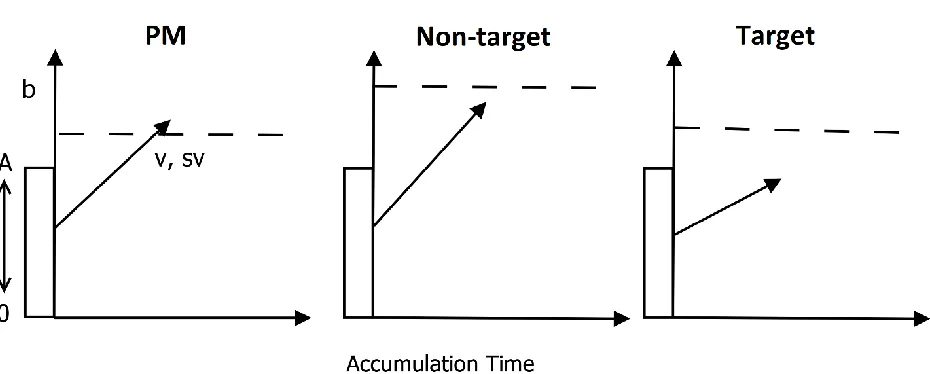
accumulator reaches threshold, determining the response made. PMDC uses three racing LBA
accumulators: two for the ongoing binary choice task responses (e.g., target and non-target) and
a third for the PM task response. This architecture, as it applies to the maritime surveillance task,
is depicted in Figure 1. The two-accumulator ongoing task variant of this model (applied to
performance in control conditions) is similar to the LBA applied by Palada et al. (2018). The
architecture models the decision-making process to each ship, with evidence accumulating
(less than four features), or is a PM ship (has both a life boat and a flag). For each decision,
evidence begins at a random start point (uniformly in the range 0-A) and increases linearly as
determined by a sample from a normal accumulation rate distribution with mean v and standard
deviation sv. Accumulation to all possible responses runs independently until one of them
reaches its threshold (b), and the first accumulator reaching threshold determines the response
made. The total time to respond includes the time for the accumulation process plus a
non-decision time constant. For each new ship for which a decision is made, evidence is reset and
another decision process runs as just described. Below we describe in detail how, when applied
to our task, the parameters of PMDC correspond to the degree of capacity sharing between PM
and ongoing task processing, as well as the degree of cognitive control over PM and
ongoing-task processes, in terms of Braver (2012)’s proactive control and reactive control.
Capacity sharing. We measure capacity sharing by comparing the accumulation rates to
non-PM items (i.e., target and non-target ships without the PM feature configuration) in PM
blocks with the accumulation rates to non-PM items in control blocks. PMDC estimates an
accumulation rate towards the correct ongoing task decision (the ‘match’ accumulation rate, e.g.,
accumulation towards the target decision for target ships), and an accumulation rate towards the
incorrect ongoing task decision (the ‘mismatch’ accumulation rate, e.g., accumulation towards
the non-target decision for a target ship). Match and mismatch accumulation may be combined
into two measures of overall processing (Palada et al., 2018), processing quality and processing
quantity. Processing quality is given by match accumulation rate minus mismatch accumulation
rate. Previous capacity sharing theories of PM cost have argued that capacity sharing would
decrease the ‘drift rate’ parameter of the diffusion decision model, which indexes quality of
sum of accumulation rates (match + mismatch). Note that decreased quantity of ongoing task
processing under PM conditions could lead to slower ongoing task decisions, and thus also may
potentially underlie the PM cost effect.
As reviewed, PM demands generally do not affect non-PM accumulation rates in simple
paradigms, in terms of either the quality or quantity of ongoing task processing. However, in
contrast to previous simple PM paradigms, the current study's demanding ongoing task may limit
available cognitive capacity. Thus, in our study, PM conditions may induce a cost to
accumulation to non-PM ships under PM conditions as compared with control conditions. This
cost may affect processing quality, quantity or perhaps both.
Proactive control. PMDC proposes that participants may apply proactive control to
increase ongoing task thresholds in PM blocks, so that when PM stimuli are presented ongoing
task decisions do not pre-empt the PM decision. PMDC also includes control over the PM
threshold, which may be adjusted based on factors such as the importance of the PM task, but
our study does not manipulate such a factor. As reviewed, many studies find evidence for
increased ongoing task thresholds in PM blocks, consistent with proactive control. Our task
differs from previous studies in that it requires time-critical ongoing-task responding. Slow
ongoing task responses can lead to failures to respond to all ships before trial deadlines, and
Palada et al. (2018) found that with increased trial load participants reduced their thresholds in an
attempt to meet trial deadlines. Therefore, if participants are concerned about non-responding,
they may avoid proactive control over ongoing task decisions in our paradigm.
Reactive control. Reactive control occurs right when a PM related event is processed, to
facilitate appropriate responding to that event. In the current context, this would be expected to
PMDC, reactive processes do not affect thresholds, because thresholds are set prior to each
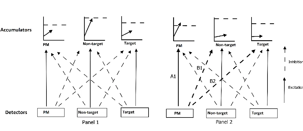
decision beginning. Instead, reactive control affects accumulation rates. PMDC’s reactive
architecture is presented in Figure 2. As PM stimulus inputs are processed, they activate
detectors for the possible decisions. For example, when PM items are processed, this can directly
excite the PM accumulator (pathway A1 in Figure 2), leading to faster PM accumulation speed
on PM items than non-PM items.
PM stimulus inputs can also inhibit the accumulation rates of ongoing task processes
(pathways B1 and B2 in Figure 2), slowing ongoing task accumulation. This reactive inhibition
would cause slower ongoing task accumulation when processing PM ships (which contain PM
stimulus input), as compared with non-PM ships. Thus, to test for reactive inhibitory control, we
compare ongoing task accumulation between PM ships and non-PM ships. Lower ongoing task
accumulation to the PM ships indicates reactive inhibition. In simple paradigms, there is strong
evidence for such reactive inhibition (Strickland et al., 2018), and it is critical to PM accuracy.
We expect to replicate these reaction inhibition findings in the current study.
Multiple stimulus processes. Each trial presents participants three stimuli they must
respond to before trial deadline (9 seconds). Although participants appear to make ongoing task
decisions one at a time in our paradigm (Palada et al., 2016), there may be initial parallel
encoding of the three ships. Moreover, participants will likely engage additional processes such
as eye saccades to orient attention to the initial ship and orienting the motor response. To allow
for this, we include a ‘response order’ factor in our analyses, which tracks whether each decision
was the first, second, or third decision made within a trial. Following Palada et al. (2018), the
model reported in text will include a different non-decision time for the first response relative to
longer for the first response than the others, and we examine whether this effect of response
order can improve overall model fit.
Method
Participants
The study was approved by the Tasmania Social Sciences Human Research Ethics
Committee. Thirty-six undergraduate students (12 females) from the University of Western
Australia and the University of Tasmania participated in the study in exchange for course credit.
Mean age was 21.6 (SD = 3.7). Due to a power failure, for one participant we did not record the
data for one half of a control block (of 120 ship presentations). Another participant closed the
program during a control block, resulting in missing data for the last 12 ships of that block. As
we collected thousands of responses per participant, we were able to include the remaining data
from these participants in all subsequent analyses. We excluded one participant from analyses
entirely because they did not make a PM response to any of the 128 PM trials over the course of
the experiment. One participant closed their practice trials early on both sessions, and another did
not respond to a high proportion of practice trials (67% session one, 32% session two).
Nonetheless, their data from the subsequent experimental trials appeared typical, so were
retained for analysis.
Materials
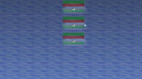
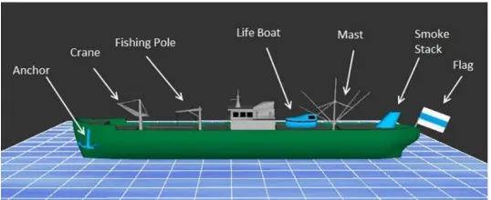
Figure 3 depicts the maritime surveillance task environment. The task display comprised
five horizontal channels of equal height. On each trial, three ships appeared and moved across
the screen from right to left. The three ships were directly above and below each other (as in
Figure 3), but the position of the group was otherwise random (i.e., the bottom ship could be in
features each ship displayed. Figure 4 shows a ship with all seven possible features. Ships with
four or more of these features were ongoing task targets, and ships with less than four of these
features were ongoing task non-targets. Above each stimulus there were red and green response
boxes, which participants left clicked to indicate their response (green for target, red for
non-target). The PM task was to make an alternate response (right click) if a ship displayed both of
two specific features (the flag and the life boat). The PM task always required right clicking the
same response box, regardless of how whether the ship was an ongoing task target or ongoing
task non-target (e.g., always right click the red response box for PM ships regardless of other
ship features). Whether PM responses were right clicks to the red or green box was
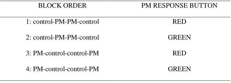
counterbalanced across participants (Table 1). We increased the difficulty of the task by
obscuring each ship with a fog cloud overlay set at 50% opacity and by adding visual noise to the
entire display.
To generate the stimuli, we created a list of all possible ships with 4 or more features
(target ship list) and a list of all possible ships with less than four features (non-target ship list).
Ship features were evenly represented across the ship lists (the ‘crane’ feature was just as likely
as the ‘mast’ feature, and so forth). Both the target and non-target ship lists were further divided
into two: PM ships (i.e., ships with both the flag and life boat features), and non-PM ships (i.e.,
ships that did not have both a flag and life boat). To fill the design as described below, ships
were drawn randomly from these lists of ships, for example, for a control block, 126 non-PM
target ships were drawn randomly from the non-PM, target ship list, and 126 non-PM non-targets
Design
Testing was split over two sessions. In each session, participants were given both PM and
control ‘blocks’ of trials. Control blocks included 252 ships (84 trials), 126 non-PM target ships
and 126 non-PM non-target ships. PM blocks included 252 ships, with 110 non-PM target ships,
110 non-PM non-target ships, 16 PM non-target ships and 16 PM target ships. Each block
included a one-minute break in the middle, to reduce possible effects of fatigue. Stimuli numbers
were split evenly across each half of the block for each stimulus type. Within each half block,
stimulus presentation order was randomized. To collect a sufficient number of PM observations,
each of the two sessions of the experiment included two PM blocks and one control block.
Across the two PM blocks we observed responses to 504 ships (168 trials), 64 of which were PM
ships (32 PM targets, 32 PM non-targets).
The two PM blocks were always presented sequentially. Thus, the order in which control
and PM blocks were presented for each session was either control-PM-PM or PM-PM-control.
Assignment of block order to session was counterbalanced across participants, resulting in two
possible block order schemes: either control-PM-PM/control or
PM-PM-control/control-PM-PM. In summary, participants were assigned to one of four conditions (see
Table 1) which determined: (1) the order in which they performed experimental blocks
(PM-PM-control vs. (PM-PM-control-PM-PM) and (2) the response button used for PM responses (red vs. green).
These factors were orthogonally counterbalanced as displayed in Table 1. Across 32 participants,
we achieved a full counterbalance: an equal distribution of subjects in each cell of our
counter-balancing scheme (with eight participants in each condition as can be seen in Table 1). Across
our two testing sites we ended up with 3 more participants than planned for, resulting in an
group 2. Our analyses below included all our data, but the conclusions held even if we excluded
the last three participants tested (for a full counterbalance).
Procedure
Training required participants to read through a slideshow of task instructions. They were
informed that they were required to classify ships as either targets or non-targets using a
7-feature classification rule. Under this rule, ships with 4 or more 7-features needed to be classified
as target by left-clicking the green response box above that ship. Ships with less than 4 features
were to be classified as non-target by left-clicking the red response button above that ship. They
were told that multiple ships would appear on-screen in adjacent positions, and that the ships
would enter and leave the screen at the same time. Participants then practiced classifying ships.
For each response, they received feedback: a red cross next to the ship for an incorrect response,
or a green tick next to the ship for a correct response (no feedback was provided in the
experimental phase). Participants completed 36 training trials (108 ships) each testing day.
After training, participants received instructions for the experimental blocks. Participants
were informed that the experimental phase would last 40 minutes. For control blocks,
participants were instructed to perform the target/non-target classification task. For the PM
blocks, participants were instructed to continue performing the target/non-target classification
task; however, they were also instructed that if a ship had both a life boat and a flag, they should
right click on the green/red response box (which depended on the counterbalance of the
participant) above the ship instead of making a left click classification response. We chose the
life boat and flag features because they were both quite distinct from the grey noise overlay
added to the task. This avoids a situation where the PM task required greater perceptual effort
ship with labels and arrows indicating the life boat and flag features (similar to Figure 4). As has
been common practice in the PM literature, we included a ‘filler’ task after the PM instructions,
before the commencement of the ongoing task. Before beginning the experimental blocks,
participants were told that they would have 2 minutes to complete a puzzle using pen and paper.
After the puzzle, they began the experimental block.
Results
Before discussing the PMDC model fits to our data, we report conventional analyses of
RTs and accuracy. Our analyses were conducted with the use of the R programming language (R
Development Core Team, 2018). We used linear mixed models, the recommended method for
repeated measures data (Pinheiro & Bates, 2000) as implemented in the R LME4 package (Bates,
Mächler, Bolker, & Walker, 2015). Post hoc analyses were performed using glht from the R
MULTCOMP package (Hothorn, Bretz, & Westfall, 2008) with Tukey adjusted p-values. We
analyzed PM condition (PM block, control block), stimulus type (non-PM target ships, non-PM
non-target ships, PM target ships, PM non-target ships), response order (response 1, response 2,
response 3) and session (session one, session two) as fixed effects, and subject as a random
effect. All responses with RT < 0.2 s (0.03%) were excluded from subsequent manifest and
model analysis.
Separate models were fit for ongoing task RTs, ongoing task accuracy, PM task RTs, PM
task accuracies, and PM false alarms. Each model was built by including each factor separately
and comparing against a null model (with subject as a random effect) to check for significant (p
<.05) improvement in model fit (using Wald chi-square tests). We built each model by stepwise
addition of each significant factor, retaining those which provided significant improvement in
chi-square tests and post hoc comparisons are provided in the supplementary materials. AIC-based
model selection yielded the same models to the method described. In text, we focus on effects
that were statistically significant, unless specified otherwise.
Ongoing task responses were scored as correct if the participant correctly identified the
stimulus. PM responses were scored as correct if the participant right-clicked the stimulus on a
PM trial. Occasionally (0.31% of responses to non-PM ships, 11.9% of responses to PM ships),
participants right-clicked a stimulus, but on the response box which they were not assigned for
their PM task (e.g., a participant told to right click green for PM right clicking red instead).
These were scored as PM responses, on the assumption that this was more likely to reflect a
procedural response error (in which participants intended to respond PM), than a PM error.
False Alarms
PM false alarms, that is PM responses to non-PM ships, occurred to 1.4% of non-PM
ships in PM blocks. The false alarm rate decreased from session one (M = 2.1%) to session two
(M = 0.6%). We observed some false alarms in control blocks (14 responses, 0.08% of the total
observed), despite participants being instructed before control blocks that they did not have to
monitor for PM items. More than half of these (8) came from a single participant. No other
participant made more than one false alarm during control blocks. As there were very few of
these false alarm responses in control blocks, they are excluded from all further analysis,
including the subsequent PMDC model fitting.
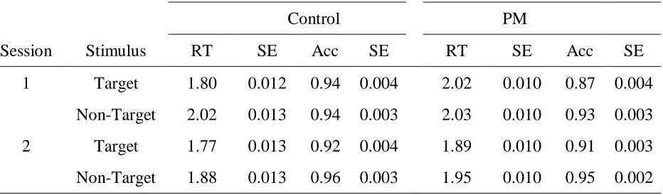
PM Costs
The results of PM cost analysis are presented in Table 2. For the ongoing task (feature
classification), correct RTs for target and non-target ships in PM blocks were longer than in
in PM blocks for both target and non-targets; however, the reduction in accuracy for targets in
the first session (7%) was substantially greater than non-targets in session one (1.3%), targets in
session two (0.8%), and non-targets in session two (0.7%). Responses to target ships were less
accurate than responses to non-targets, except for the control block in the first session, where
there was no significant difference in accuracy between target and non-target ships.
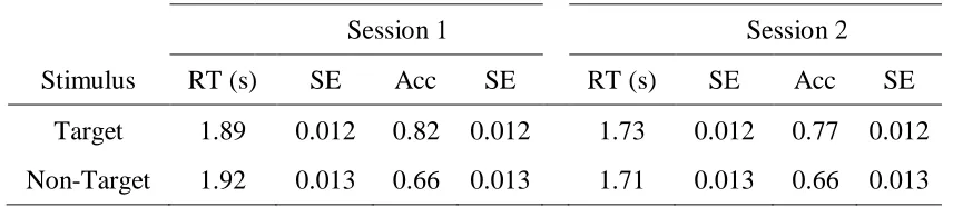
PM Task Performance
Other than response order (which will be covered in the next section) only “session”
affected correct PM RTs, which decreased from the first session (M = 1.90, SE = .03) to the
second session (M = 1.72, SE = .03). PM task accuracy for targets and non-targets is shown in
Table 3. PM accuracy was higher for target ships than for non-target ships both sessions. PM
accuracy to target ships decreased from session one to session two.
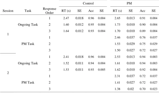
Response Order
To determine whether response order within a trial affected performance, we compared
correct RTs and accuracy of the first, second and third responses. RTs and accuracies by
response order are presented in Table 3. For the ongoing task, the first RT on each trial was
longer in both control and PM conditions, but there was no significant difference in RTs between
the second and third response in either session. For the PM task, correct RTs followed a similar
pattern to the ongoing task: the first response took substantially longer, but there was no
difference in RT between the second and third response. For the ongoing task, accuracy
and second ongoing task response did not significantly differ. Overall, response order did not
affect PM accuracy.
Consistent with the higher mean RT on the first response of each trial, we suspected that
individuals were engaging in additional non-decisional processes at the start of each trial (Palada
et al., 2018), as a result of parallel encoding of stimuli, motor response orientation and eye
saccades. In order to justify the inclusion of a separate non-decision time parameter for the first
response in the subsequent PMDC modeling, we first checked for further differences in the
manifest data, by examining the 0.1 quantiles of RT for each participant. Because non-decision
time is a constant time added to each trial, the fastest responses (i.e., those with relatively small
decision times), should be sensitive to shifts in non-decision time. We found that the 0.1
quantiles of RTs were longer for the first responses on each trial (M = 1.17, SE = .016) relative to
other responses, suggesting that we should include a difference in non-decision time in
subsequent model analysis. In contrast, there was only a small difference between the second (M
= 0.95, SE = .003) and third (M = 0.94, SE = .003) responses.
To conclude, we found PM costs not only to ongoing task RT, but also to ongoing task
decision accuracy. This is consistent with findings from PM in simulations of air traffic control
(e.g., for a review see Loft, 2014). These data suggest that our simulation of maritime
surveillance is sufficiently cognitively demanding to place participants in the ‘red zone’, in
which PM monitoring and ongoing task performance must trade-off. In contrast to previous
studies, our design is sufficiently high powered and controlled to also apply the PMDC model,
which allows us examine the cognitive control and capacity related mechanisms that underlie
Model Results
We apply the PMDC model, as described in the introduction and depicted in Figure 1.
We report thresholds in terms of B > 0 (equal to b - A). Our design included several factors that
parameters could conceivably vary over: PM condition (control vs PM), stimulus type, latent
response accumulator (non-target, target, PM), response order, and session of experiment. In
order to constrain the flexibility of the model so that it would remain a ‘measurement model’
with parameters that can be accurately estimated from the data, we applied several a priori
constraints on which parameters were allowed vary with design factors.
We constrained A to be the same across all accumulators and all conditions. To account
for the possibility that participants took extra time to encode the locations of the three ships in
parallel, and to orient their attention and motor response (mouse cursor) to the first ship, we
allowed a different non-decision time for the first response in each trial relative to the other
response orders. Consistent with Palada et al. (2018), we did not allow any additional flexibility
over response order, as doing so would risk too little data for acceptable parameter estimation
(recall that we only observe responses to 64 PM target ships and 64 PM non-target ships for each
participant). We fixed non-decision time over all other factors. We estimated thresholds
separately for each accumulator, for each PM condition (PM vs. control), and for each session of
the experiment. Following results and precedent from simple laboratory paradigms (Strickland et
al., 2017, 2018), we relied on thresholds alone to capture the effects of session. We did not
estimate separate thresholds in response to stimulus type. As stimuli were randomly presented,
estimating thresholds based on stimulus type would be circular: if participants could change
adjust thresholds in contingent on stimulus identity, then they must have already known what
accumulation rates to vary over PM condition and stimulus type. As is common in applications
of the LBA, we included only two accumulation rate standard deviations: a ‘matching’ standard
deviation parameter for correct decisions and ‘mismatching’ standard deviation parameter for
errors. We fixed the standard deviation of the ‘mismatch’ accumulator at 1, so that the model
was identifiable (Donkin, Brown, & Heathcote, 2009). From these aforementioned constraints,
the ‘top’ most flexible model we fit comprised 29 free parameters – one start-point noise
parameter, 10 thresholds, 15 mean accumulation rates, 1 standard deviation for ‘match’
accumulation rates, and 2 non-decision times.
Sampling
We estimated model parameters using Bayesian estimation, which produces a probability
distribution for each parameter value. We used the Differential Evolution Markov Chain Monte
Carlo algorithm (DE-MCMC; Turner, Sederberg, Brown, & Steyvers, 2013), an algorithm that is
effective in Bayesian estimation even when parameters are highly correlated, as implemented in
the DMC suite of R functions (Heathcote et al., in press). Bayesian estimation requires
specifying ‘prior’ distributions, which specify beliefs about parameter values prior to modelling
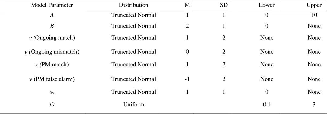
the data. As this was the first application of PMDC to our task, we specified fairly
non-informative priors, which are listed in Table 1. Our priors were similar to the priors used by
Strickland et al., (2018). However, in order to account for the longer RTs observed in our task,
we doubled the prior means of the B parameters (the amount of evidence required for a decision)
and increased the upper bound on non-decision time to 3 seconds.
The DE-MCMC algorithm requires running many parallel chains, which share
information to efficiently converge to the posterior distribution. We ran three times as many
reduce computational requirements, we ‘thinned’ during sampling, only retaining one out of
every twenty iterations that we ran. We ran 3600 iterations at a time, retaining 180 of them after
thinning. We continued to run more iterations (replacing the samples from the previous 180)
until all samples were stationary, mixed, and converged, which we evaluated both with Gelman’s
𝑅̂ statistic (Gelman et al., 2014) and with visual examination of trace plots of the samples.
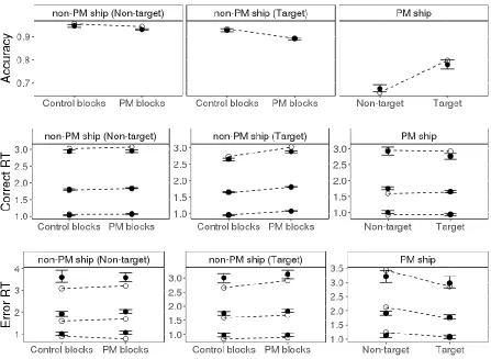
Model Fit
Before interpreting the model, we examine whether it adequately accounts for the
observed data, using graphs of ‘posterior predictive’ (Meng, 1994) model fit. This involves using
the posterior parameter samples to simulate data from the model and comparing them with the
actual data. Figure 5 compares the fit between simulated and observed data across the different
PM conditions, stimulus types, and responses. Overall, the PMDC architecture provided a good
fit to accuracies and RTs of the ongoing task and of the PM task. We separately examined fit to
the ‘response order’ factor, depicted in Figure 6. The model adequately captures the major effect
of ‘response order’ on RT. There is some miss-fit to the extended tail of RTs for response order
one, and slight miss-fit for some of the accuracy trends. Although this miss-fit may be addressed
with more parameters1, it is not very substantial, and we decided that further gains in fit to our
data would not be worth the added model complexity (i.e., more potential to over-fit to noise in
our data and thus not generalize well to future data). Next, we describe how the model achieved
good fits to our observed data in terms of latent psychological quantities. To do so, we first
explore the possibility of constraining the model further with model selection.
1 We experimented with more complex models (e.g., thresholds and rates varying by trial position, 78 parameters)
Model Selection
In addition to the a priori constraints on the model, we tested whether the deviance
information criterion (DIC; Spiegelhalter, Best, Carlin, & Van Der Linde, 2002) suggested any
further constraint would be appropriate. DIC measures how ‘good’ a model is by considering
both complexity and goodness of fit to the data. A lower DIC indicates a better model. DIC
values were summed across participants. We tested three models. The first was the ‘top’, most
flexible model, that allowed both capacity sharing and proactive control in the PM and control
conditions. The top model had 29 parameters and a DIC value of 110468. We tested an ‘only
capacity sharing model’, in which thresholds were fixed across PM conditions, precluding
proactive control. Although this model was simpler, with only 25 parameters, it had a
substantially larger DIC than the top model (DIC difference = 1140), indicating support for the
top model. We tested an ‘only proactive control’ model, in which accumulation rates to non-PM
stimuli did not vary across PM and control conditions. This model had 25 parameters and was
also rejected in favor of the top model, (DIC difference = 322), suggesting that changes in
non-PM accumulation rates were required to fit the data. Thus, overall, the model selection is in favor
of both thresholds and rates varying across PM and control blocks. We now test the direction and
magnitudes of these variations in thresholds and rates.
Model Summary
Parameters
To summarize model parameters, we created a group-averaged posterior distribution,
which averaged every posterior sample across participants. To test differences between
parameters, we took the differences between the parameters for each posterior sample, and then
To summarize the difference distributions, we report the proportion of posterior samples of the
difference that were above or below 0 (p). So that p values are consistent (with smaller ps
evidencing an effect), we report the posterior p against effects running in the observed direction.
Thus, if a tested difference in parameters is most often sampled above 0, we report the p that it is
below 0, and if a difference is most often sampled below 0, we report the p that it is above 0. We
also report Z, the mean of the difference distribution divided by the standard deviation (similar to
a Z score because the difference distributions of posterior samples are approximately normal).
We include the latter because many of our observed effects were ‘significant’ in that p = 0, and
so we needed some way to compare their relative size. For t0, we found an effect of position in
trial, with the t0 to the first response on each trial much higher (M = 0.77s, SD =0.004) than t0 to
the subsequent two (M = 0.12s, SD = 0.003s), Z = 222.7, p = 0. This non-decision time effect is
consistent with greater encoding time at the start of each trial, in which participants have to
locate the three ships, and perhaps have to move their mouse to the first ship. The values of
non-decision time are similar to those reported by Palada et al., (2018). The posterior mean of the
standard deviation in rates for the matching accumulator was 0.65 (SD = 0.01). As the standard
deviation for the mismatching accumulator was fixed at 1, this replicates most previous modeling
with the LBA where the match accumulator is generally found to have lower variability than the
mismatching accumulator. The posterior mean of the A parameter was 2.71 (SD = 0.05).
Capacity Sharing
We tested capacity sharing by comparing accumulation rates to non-PM ships across
control blocks and PM blocks, with slower non-PM accumulation in PM blocks indicating
capacity sharing. Figure 7 shows the accumulation rates for non-PM ships broken down by
for the matching accumulator was lower for targets in PM blocks (M = 2.32, SD = 0.03) than in
control blocks (M = 2.48, SD = 0.03), Z = 7.37, p = 0 (top right panel). Although the effect was
smaller, the rate for the matching accumulator was also lower for non-targets in PM blocks (M =
2.25, SD =0.03) than control blocks (M = 2.30, SD =0.03), Z = 2.45, p = .007 (top left panel).
The rate for the mismatching accumulator was not appreciably different in PM blocks (M
= -0.30, SD = 0.05) than control blocks (M= -0.33, SD = 0.06), Z = 0.36, p = .361, when targets
were presented (bottom right panel). However, the rate for the mismatching accumulator was
marginally higher for non-targets in PM blocks (M = -1.07, SD = 0.07) than control blocks (M =
-1.22, SD = 0.08), Z =1.6 p = .06 (bottom left panel).
We also combined the rate measures to test changes across condition in processing
quality (match accumulation – mismatch accumulation) and processing quantity (match
accumulation + mismatch accumulation) for non-PM ships. We found lower processing quality
under PM conditions for both targets, Z = 2.66, p = .004, and non-targets, Z = 2.06, p = .02. We
found lower processing quantity for targets, Z = 1.98, p = .03, but not non-targets, Z = -1.08, p =
.14. Overall then, with three effects on accumulation rates consistent with lower ongoing task
capacity, and one rate not affected by PM condition, these results suggest lower ongoing capacity
in PM blocks than control blocks. These effects were modest in size compared to some other
effects in the model, but in the ‘Model Exploration’ section we will demonstrate that they were
important in accounting for PM costs.
Proactive Control
To test for proactive control, we compared ongoing task thresholds in PM blocks with
control blocks; with higher ongoing task thresholds in PM blocks being indicative of proactive
PM blocks (session one M = 2.32, SD = 0.03, session two M = 2.03, SD = 0.03) than control
blocks (session one M= 2.00, SD = 0.03, session two M = 1.91, SD = 0.03) for both session one,
Z = 10.92, p = 0, and session two, Z = 4.38 p = 0. Proactive control over non-target decisions was
less apparent. In session one, thresholds to make non-target decisions were not higher in PM
blocks (M = 2.21, SD =0.03) than control blocks (M = 2.21, SD = 0.04), Z = 0.16, p = .434.
However, in session two, non-target thresholds were higher in PM blocks (M = 2.04, SD = 0.03)
than control blocks (M = 1.91, SD = 0.03), Z = 4.69 p = 0. Thresholds towards the PM decision
were not substantially higher for session one (M = 1.73, SD = 0.04) than for session two (M =
1.73, SD = 0.04), Z = 0.28, p = .39.
Reactive Control
Excitation. In order to examine reactive processes, we compare differences in
accumulation between PM ships and non-PM ships. Trivially, as would be expected with
reasonable PM accuracy, PM accumulation was substantially faster to PM ships (target ships M=
2.14, SD = 0.04, and non-target ships M =1.70, SD = 0.04) than to non-PM ships (M = -3.79, SD
= 0.12), Z = 52.64, p =0. More interestingly, PM excitation was greater to ‘target’ PM ships (PM
ships that also satisfy the ongoing task target detection rule), than to ‘non-target’ PM ships (PM
ships that do not satisfy the ongoing target detection rule), Z = 11.5, p = 0.
Inhibition. We tested for reactive inhibition by comparing ongoing task accumulation
rates between PM ships and non-PM ships. These rates are plotted in Figure 9. Lower ongoing
task accumulation to PM ships indicates inhibition. For target ships, accumulation towards the
decision to respond 'target' was much lower when the target was a PM ship (M = 0.61, SD =0.08)
than when it was a non-PM ship (M = 2.32, SD =0.03), Z = 24.79, p = 0 (top right panel, Figure
much lower when the non-target was a PM ship (M = 0.88, SD = 0.05) than when it was a
non-PM ship (M = 2.25, SD = 0.03), Z = 29.64, p = 0 (top left panel). For target ships, there also was
evidence that the error accumulation rates were lower when the target was a PM ship (M = -1.56,
SD = 0.15), than when it was a non-PM ship (M = -0.30, SD = 0.05), Z = 8.18, p = 0 (bottom
right panel). For non-target ships, error accumulation was also lower when the non-target was a
PM ship (M = -1.44, SD = 0.14) than when it was a non-PM ship (M =-1.07, SD = 0.07), Z =
2.53, p = .004 (bottom left panel).
We also examined inhibition in terms of processing quality and processing quantity. For
target ships, ongoing task processing quality was lower for PM ships than non-PM ships, Z =
2.64, p = .005. For non-target ships, ongoing task processing quality was lower for PM ships
than non-PM ships, Z = 6.5, p = 0. For target ships, ongoing task processing quantity was much
lower for PM ships than non-PM ships, Z = 17.58, p = 0. This was also the case for non-target
ships, Z = 11.36, p = 0.
Model Exploration
In complex cognitive models, the contribution of model processes to the observed data
can be difficult to discern. Here, we seek to understand the model processes that underlie PM
cost and accuracy by removing them from the model and examining the miss-fit to PM cost and
PM accuracy that follows. To the extent that removing a model mechanism causes miss-fit to an
effect, that effect can be ascribed to the mechanism in the full model. We summarize model fit
by examining the percentages of PM accuracy and PM cost predicted. This percentage can be
over 100 if the model actually predicts a larger number than the data.
PM accuracy. First, we tested the contributions of proactive and reactive control to PM
the model by setting thresholds in PM blocks to control block levels (removing proactive control
of ongoing tasks decisions), and also setting ongoing task accumulation rates on PM ships to the
level on non-PM ships (removing reactive control). Whereas the full model predicted 98% of PM
accuracy to target ships and 103% of accuracy to non-target ships, the model with control
removed predicted only 59% of accuracy to target ships, and 65% to non-target ships. Next, we
examined a model with proactive control in the model, but not reactive control. This predicted
65% of PM accuracy to target ships, and 66% of accuracy to non-target ships indicating that
proactive control made some contribution to PM accuracy in the full model. However, allowing
reactive control into the model, but not proactive control, resulted in much better fits to PM
accuracy, with 95% of PM accuracy predicted to target ships and 100% of accuracy predicted to
non-target ships. This illustrates that for the current task, proactive control had relatively little
influence on PM accuracy, whereas reactive inhibitory control was critical.
PM cost. Next, we tested the extent to which the PM cost effect could be accounted for
by proactive control compared to capacity sharing. We examined a model with proactive control
removed by setting all ongoing task thresholds to the values in control conditions; and we
examined a model with capacity sharing removed by setting all non-PM accumulation rates to
the values from control blocks. The results are displayed in Figure 11. We only discuss cost to
responses to target ships, because cost to non-target ships was small, and the 95% credible
intervals of all the models overlapped with the true effect. The full model predicted 104% of cost
to target ships, whereas removing capacity sharing resulted in predicting only 54% of cost to
target ships. Similarly, removing proactive control predicted only 39% of cost to target ships.
These results suggest that both capacity sharing and proactive control played substantial roles in
Individual Differences in PM Accuracy
We were also interested in how the model explained variation in PM accuracy across
participants. We investigate this by correlating model mechanisms with PM accuracy. To obtain
correlations, we calculated model mechanisms (e.g., proactive control over target decisions) for
each posterior sample for each participant, and then calculated the correlation for that posterior
sample. The result is a distribution of posterior correlations (Ly, Boehm, et al., 2018). We
applied a correction to the correlations, so that they are suitable for inference about the
population rather than the sample (Ly, Marsman, & Wagenmakers, 2018). We plot the posterior
means, and credible intervals, of the resulting correlation distributions in Figure 12. Below we
report in text the posterior means of the substantial correlations.
In our previous work using a simple paradigm, we found that only reactive inhibition
towards the ‘match’ ongoing task decision strongly correlated with PM accuracy. We replicated
this reactive inhibition effect here, for PM accuracy both to target PM ships (r = .74) and to
non-target PM ships (r = .73). Furthermore, reactive inhibition to the target response for
non-targets was correlated with target PM accuracy (r = .55), and reactive inhibition of the target
response to target PM ships was correlated with non-target PM accuracy (r = .57). These
correlations suggest that reactive control ability is a strong determinant of individual differences
in PM accuracy.
We found another parameter that correlated with PM accuracy here that did not correlate
in the simple PM paradigm: the PM accumulation rate. The speed of PM accumulation correlated
with PM accuracy both to target PM ships (r = .55) and non-target PM ships (r = .82).
accuracy to target PM ships (r = .62) and the PM accumulation rate towards target PM ships was
correlated with PM accuracy towards non-targets (r = .49).
Multiple Stimulus Encoding
In each trial, participants were presented three ships and were instructed to respond to in
any order they wished. As reviewed above, we found substantially slower responses for the first
ship on each trial, consistent with Palada et al. (2018). This motivated a subsequent analysis of
our manifest data. Although it is unlikely that participants would switch their attention between
the ships during decisions (Palada et al., 2016), it is possible that at the beginning of each trial,
prior to focusing attention on the first ship (and performing evidence accumulation), participants
might either perform some initial scan of the ships for PM features, or notice the PM features
during initial encoding of the locations of the three ships. We tested this for each participant by
performing a chi-square test on the frequency with which PM items were responded to first. As
PM ships were interspersed randomly amongst the other ships, the null hypothesis was that PM
ships would be responded to first no more than chance. The null was calculated for each
participant by examining the total number of responses recorded first, second, and third within a
trial (this was not exactly a third due to non-responses, although very close). We tabulate the
results of the chi-square tests for each participant in the supplementary materials.
We found four participants who responded to PM ships first more often than chance (p
less than the family-wise error rate of .0014). This motivated two checks of our model results.
First, we checked whether the inferences reported above held without the four ‘PM first’
participants included in the data, and we found that they did. Second, we examined non-decision
times of the four ‘PM first’ participants compared with the rest of the participants. We found that
(M = 0.84s, SD = 0.009s) than other participants (M = 0.76s, SD = 0.004s), Z = 7.46, p = 0,
whereas the non-decision times for the other two responses were slightly faster for the four
participants (M = 0.11s, SD = 0.004s) than for the rest of the sample (M = 0.12s, SD = 0.003s), Z
= 2.99, p = .006. Given these results, it is possible that participants who encode stimuli more
thoroughly at the beginning of the trial can notice PM ships during encoding, and then
subsequently orient their attention to a PM ship first for that trial.
Discussion
In the current study, we examined PM in a laboratory simulation of a complex, dynamic,
maritime surveillance task. We found substantial PM error rates in our task, similar to those
observed in simple laboratory paradigms (Einstein & McDaniel, 1990). Replicating findings
from simple laboratory PM tasks, we found a PM cost to RT of the ongoing target detection task.
Specifically, in PM blocks of trials we found slower RTs to (non-PM) ongoing task targets. We
also found a PM cost to ongoing-task target accuracy. We used our data to test the recently
developed PMDC model (Strickland et al., 2018). We found that PMDC fitted well to the
observed performance data, despite the RTs in this task being much slower than in tasks PMDC
has previously been applied to. This finding corroborates other recent studies that have
successfully validated accumulation models in tasks that require longer decisions, and thus are
more representative of decisions in complex real-world task environments (Lerche & Voss,
2017; Palada et al., 2016, 2018). Critically, we found that PMDC was applicable to, and
informative about, human performance in a ‘red zone’ of task demand. PMDC indicated capacity
sharing between PM monitoring and ongoing task performance, contrasting with previous
findings from simple paradigms that PM monitoring does not impact ongoing task capacity