This is a repository copy of
Long memory estimation for complex-valued time series
.
White Rose Research Online URL for this paper:
http://eprints.whiterose.ac.uk/132566/
Version: Accepted Version
Article:
Knight, Marina Iuliana orcid.org/0000-0001-9926-6092 and Nunes, Matthew A. (2018)
Long memory estimation for complex-valued time series. Statistics and computing. pp.
1-20. ISSN 0960-3174
https://doi.org/10.1007/s11222-018-9820-8
[email protected] https://eprints.whiterose.ac.uk/
Reuse
This article is distributed under the terms of the Creative Commons Attribution (CC BY) licence. This licence allows you to distribute, remix, tweak, and build upon the work, even commercially, as long as you credit the authors for the original work. More information and the full terms of the licence here:
https://creativecommons.org/licenses/
Takedown
If you consider content in White Rose Research Online to be in breach of UK law, please notify us by
(will be inserted by the editor)
Long memory estimation for complex-valued time series
Marina I. Knight · Matthew A. Nunes
Received: date / Accepted: date
Abstract Long memory has been observed for time series across a multitude of fields and the accurate es-timation of such dependence, e.g. via the Hurst ex-ponent, is crucial for the modelling and prediction of many dynamic systems of interest. Many physical pro-cesses (such as wind data), are more naturally expressed as a complex-valued time series to represent magni-tude and phase information (wind speed and direction). With data collection ubiquitously unreliable, irregular sampling or missingness is also commonplace and can cause bias in a range of analysis tasks, including Hurst estimation. This article proposes a new Hurst expo-nent estimation technique for complex-valued persis-tent data sampled with popersis-tential irregularity. Our ap-proach is justified through establishing attractive theo-retical properties of a new complex-valued wavelet lift-ing transform, also introduced in this paper. We demon-strate the accuracy of the proposed estimation method through simulations across a range of sampling scenar-ios and complex- and real-valued persistent processes. For wind data, our method highlights that inclusion of the intrinsic correlations between the real and imag-inary data, inherent in our complex-valued approach, can produce different persistence estimates than when using real-valued analysis. Such analysis could then sup-port alternative modelling or policy decisions compared with conclusions based on real-valued estimation.
M. I. Knight
Department of Mathematics, University of York, Heslington, York, YO10 5DD, UK
E-mail: [email protected]
M. A. Nunes
Department of Mathematics and Statistics, Fylde College, Lancaster University, Lancaster, LA1 4YF, UK
E-mail: [email protected]
Keywords complex-valued time series · Hurst exponent·irregular sampling·long-range dependence·
wavelets
1 Introduction
Complex-valued time series arise in many scientific fields of interest, for example digital communication and sig-nal processing (Curtis, 1985; Martin, 2004), environ-mental series (Gonella, 1972; Lilly and Gascard, 2006; Adali et al, 2011) and physiology (Rowe, 2005). Mod-elling and analysis of such series in the complex do-main is not only natural, but also convenient. In addi-tion, complex-valued time series models are often able to represent more realistic behaviour in observed physi-cal processes, see e.g. Mandic and Goh (2009); Sykulski et al (2017). A particular modelling aspect which has received recent attention is the property ofimpropriety
ornoncircularity, describing series whose statistics are not rotationally invariant in the complex plane (for a precise definition, the reader is directed to Sykulski and Percival (2016)). Such models of improper processes have seen growing interest in the statistics community, see e.g. Schreier and Scharf (2003); Rubin-Delanchy and Walden (2008); Mohammadi and Plataniotis (2015). Furthermore, complex-valued analysis ofreal-valueddata has been shown to be beneficial in a number of set-tings, see e.g. Olhede and Walden (2005); Hamilton et al (2017). For a comprehensive introduction to complex-valued signals, we refer the reader to Schreier and Scharf (2010); see Adali et al (2011) and Walden (2013) for re-cent advances in modelling complex-valued signals.
which has seen extensions of real-valued process mod-elling frameworks for the complex-valued fractional Brownian motion (fBM) and Mat´ern processes, see re-spectively Coeurjolly and Porcu (2017b) and Lilly et al (2017), as well as for (improper) fractional Gaussian noise (Sykulski and Percival, 2016). For these construc-tions, just as for real-valued processes (Hurst, 1951; Mandelbrot and Van Ness, 1968), the degree of memory can still be quantified by means of a single parameter, the Hurst exponent parameter (Amblard et al, 2012; Sykulski and Percival, 2016). Accurate estimation of the Hurst parameter offers valuable insight into a mul-titude of modelling and analysis tasks, such as model calibration and prediction (Beran et al, 2013; Rehman and Siddiqi, 2009; Knight et al, 2017).
Complex-valued processes, both proper (circular) and improper (noncircular), are relevant across fields such as oceanography and geophysics (Adali et al, 2011; Sykulski et al, 2017), where data are typically diffi-cult to acquire and will frequently suffer from omis-sions/ missingness or be irregularly sampled (see e.g. Figure 1). In the next section, we describe datasets aris-ing in environmental science that feature missaris-ing obser-vations, which can be examined for long memory with a complex-valued representation. However, we note here that data from other scientific areas may benefit from analysis with our proposed methodology, see Section 6 for further discussion.
1.1 Persistence in wind series
Our motivating data example in this article arises from climatology. More specifically, wind series have been analysed extensively in the literature for modelling lo-cal weather patterns and spread of pollutants, as well as global climate dynamics. Long memory in wind series has been established by a number of authors, see e.g. Haslett and Raftery (1989); Chang et al (2012); Piac-quadio and de la Barra (2014) and references therein. Specifically, Hurst exponent estimates for wind speed series on a range of sampling resolutions, including the five minute scale considered here, have been shown to be in the range 0.7−0.9, indicating strong long-range de-pendence, see e.g. Fortuna et al (2014). Accurate Hurst exponent estimation is used for accurate forecasting of wind speed, for example to assess future power yields (Haslett and Raftery, 1989; Bakker and van den Hurk, 2012).
Wind speed analysis in the literature is predomi-nantly performed using real-valued data, such as (mag-nitude) wind speed series. However, more recently a number of authors have advocated modelling wind mea-surements ascomplex-valued, developing analysis tools
which exploit both speed and directional information of wind time series, see e.g. Goh et al (2006); Tanaka and Mandic (2007). These complex-valued modelling approaches have resulted in methodology for improved prediction for series such as those considered in this article (Mandic et al, 2009; Dowell et al, 2014). To our knowledge,long memory estimationfor stationary time series is exclusively performed using real-valued time se-ries. In this article, we analyse the degree of persistence (long memory intensity) exhibited by complex-valued wind measurements, i.e. series which have both wind speed and direction, using new complex-valued Hurst estimation methodology we propose here.
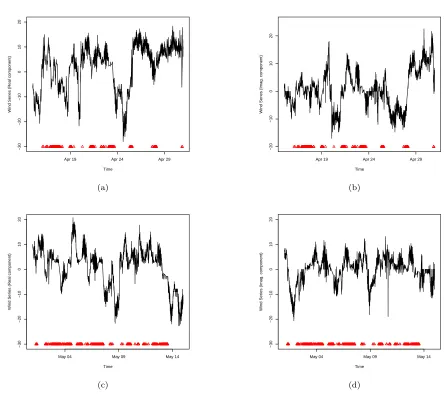
The wind series we consider in this article consists of two datasets measured at a five minute resolution from the Iowa Department of Transport’s Automated Weather Observing System (AWOS). The (speed and angular) measurements for both datasets are available athttp://mesonet.agron.iastate.edu/AWOS/. We firstly analyse data obtained from the Atlantic Munic-ipal Airport (AIO) monitoring site over a period from 15th April 2017 until 30th April 2017. Whilst the sam-pling interval for the measurements is reported as five minutes, due to a number of reasons, for example faulty recording devices, the data in fact feature missingness which results in a mix of sampling intervals – our first dataset has intervals ranging from 5 to 15 minutes.
Since we have both speed and directional informa-tion for the dataset, we shall view the series using a complex-valued representation. The real and imaginary components of the series are shown in Figure 1(a) and Figure 1(b), together with the locations of the missing data (depicted by triangles). The length of the first se-ries is n= 3131 with an overall rate of missingness of 12%. Similar datasets from the Iowa monitoring sys-tem have been previously studied in the literature for the non-missing case but not in the context of Hurst estimation, see e.g. Tanaka and Mandic (2007); Adali et al (2011).
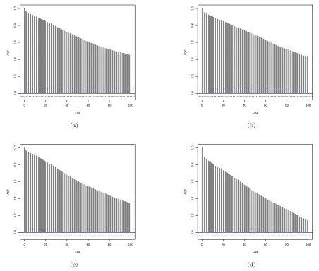
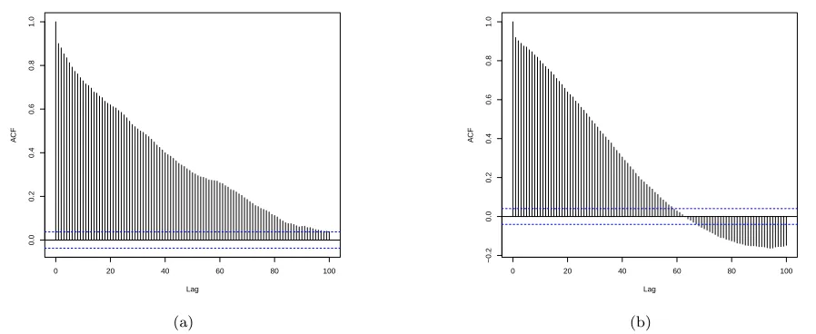
To explore the potential persistence in wind series, we examine the autocorrelation in the real and imagi-nary parts of the series, shown in Figure 2(a) and Fig-ure 2(b) for theWind Aseries. For these data, both com-ponents show highly significant autocorrelation over a range of lags, indicating long memory.
Apr 19 Apr 24 Apr 29
−30
−20
−10
0
10
20
Time
Wind Ser
ies (Real component)
(a)
Apr 19 Apr 24 Apr 29
−20
−10
0
10
20
Time
Wind Ser
ies (Imag. component)
(b)
May 04 May 09 May 14
−30
−20
−10
0
10
20
Time
Wind Ser
ies (Real component)
(c)
May 04 May 09 May 14
−30
−20
−10
0
10
20
Time
Wind Ser
ies (Imag. component)
(d)
Fig. 1: (a) Real component of theWind Adata series; (b) Imaginary component of theWind Adata series; (c) Real component of the Wind Bdata series; (d) Imaginary component of theWind Bdata series. Red triangles indicate missing data locations.
between 10 and 20 minutes resulting from a missingness proportion of 20%; the series is of lengthn= 2942. We have specifically chosen to examine this second time period due to its high degree of missingness. The two components of the complex-valued series can be seen in Figure 1(c) and Figure 1(d) (triangles indicate missing series values).
Similar observations about potential long memory characteristics can be made for the second complex-valued wind series. In particular, both real and imagi-nary components of the series show considerable auto-correlation over a large range of lags (Figure 2(c) and Figure 2(d)).
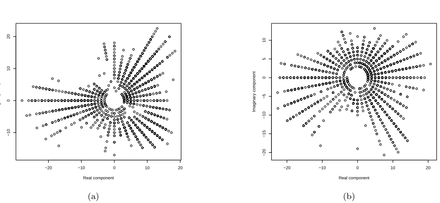
In addition, plotting the series in the complex plane, we see that both datasets exhibit a rotational behaviour, due to the angular component of the series (Figure 3).
The series are not symmetric, exhibiting clear noncircu-larity, suggesting a model which allows for impropriety is appropriate for analysis (for an in-depth discussion of these properties the reader is directed to e.g. Sykulski and Percival (2016)). This reflects similar observations on impropriety shown for other Iowa AWOS data in Adali et al (2011), as well as other wind series (Mandic and Goh, 2009).
1.2 Aim and structure of the paper
[image:4.595.60.504.93.487.2]so-0 20 40 60 80 100
0.0
0.2
0.4
0.6
0.8
1.0
Lag
A
CF
(a)
0 20 40 60 80 100
0.0
0.2
0.4
0.6
0.8
1.0
Lag
A
CF
(b)
0 20 40 60 80 100
0.0
0.2
0.4
0.6
0.8
1.0
Lag
A
CF
(c)
0 20 40 60 80 100
0.0
0.2
0.4
0.6
0.8
1.0
Lag
A
CF
(d)
Fig. 2: (a) Autocorrelation for (a) the real component of the Wind A series from Figure 1; (b) the imaginary component of the Wind A series; (c) the real component of the Wind B series from Figure 1; (d) the imaginary component of the Wind B series (all treated as regularly spaced). Both components of the two datasets show autocorrelation at large lags, indicating persistent behaviour.
lution is to combine the two pieces of information into a single, complex-valued series and analyse its proper-ties (Mandic and Goh, 2009). Adopting this approach thus calls for analysis techniques capable of dealing with complex-valued data. Additionally, for many applica-tions the process sampling structure is inherently ir-regular, as the two components may be measured at irregular times, or the data may be blighted by miss-ingness due to measurement device failures. In the real-valued case, the common practice of preprocessing the data to mitigate against irregular or missing observa-tions, results in inaccuracies in long memory estimation by traditional methods. More specifically, there is now well-documented evidence that preprocessing by impu-tation or interpolation, as well as data aggregation leads
to overestimation of persistence, see for example, Beran et al (2013), Zhang et al (2014) or Knight et al (2017). In practice, to the authors’ best knowledge, the only technique that permits Hurst exponent estimation for complex-valued processes is that of Coeurjolly and Porcu (2017b) which tackles the setting of regularly sampled (proper) complex-valued fractional Brownian motion. Motivated by the serious implications of inaccurate es-timation in the real-valued setting, in this work we pro-pose the first methodological approach that answers the timely challenge of accurate assessment of long mem-ory persistence for complex-valued processes featuring regularor irregular sampling (including missingness).
[image:5.595.58.510.103.487.2]−20 −10 0 10 20
−10
0
10
20
Real component
Imaginar
y component
(a)
−20 −10 0 10 20
−20
−15
−10
−5
0
5
10
Real component
Imaginar
y component
[image:6.595.71.504.87.287.2](b)
Fig. 3: Scatter plot of real and imaginary series values for (a) theWind Adata and (b) theWind Bseries shown in Figure 1. Both series exhibit noncircular (improper) characteristics.
choice is two-fold: (i) (classical) wavelets have proved to be very successful in the context of regularly sampled (real-valued) time series with long memory and are con-sidered the ‘right domain’ of analysis (Flandrin, 1998); and (ii) for irregularly sampled (real-valued) processes, or those featuring missingness, the wavelet lifting algo-rithm of Knight et al (2017) has provided a first long memory estimation solution and was shown to yield competitive results even for regularly sampled data.
The main contributions of the work in this paper are as follows. We propose (1) a novel lifting algorithm designed to work on complex-valued data with a po-tentially irregular sampling structure and (2) a Hurst parameter estimator for complex-valued processes sam-pled with a regular or irregular structure. Our method will be shown to improve on real-valued Hurst estima-tion results, including for regularly spaced data.
The remainder of this article is organised as fol-lows. We begin, in Section 2, by reviewing (complex-valued) long memory processes and giving an overview of wavelet lifting transforms. Section 3 introduces our novel complex-valued lifting transform, establishes its iterative bases construction and theoretical results on its decorrelation properties. Section 4 demonstrates how these properties can be exploited to design our proposed lifting-based Hurst exponent estimation procedure for complex-valued data sampled with irregularity/ miss-ingness. Section 5.1 contains a simulation study eval-uating the performance of our new method using syn-thetic data. In Section 5.2, we consider the application of our approach to the wind series datasets introduced in Section 1.1, discussing the potential consequences of
our analysis. Finally, Section 6 outlines some avenues of future work and discusses other potential applications.
2 Review of complex-valued processes, long-range dependence and wavelet lifting
2.1 Complex-valued processes
Let us denote a (complex-valued) second-order station-ary time series by {Xt} and its autocovariance func-tion asγX(ti−tj) =E(XtiXtj), under the assumption thatE(Xt) = 0 and denoting by·complex conjugation. As the autocovariance functionγX does not completely characterise a complex-valued time series, we also make use of its complementary or pseudo-covariance,rX(ti−
tj) =E(XtiXtj), again assumingE(Xt) = 0. In general, both autocovariances are complex-valued and have the properties of Hermitian symmetry and symmetry, re-spectively (see e.g. Sykulski and Percival (2016)).
In many applications, such as radar and communica-tions, processes are assumed to have the property that
real-valued autocovariances, which is precisely the set-ting under which Sykulski and Percival (2016) develop their exact simulation method for improper stationary Gaussian processes.
2.2 Long memory and its estimation
Classical literature for long-range behaviour of real-valued processes shows that persistence is often charac-terized by a parameter, such as the Hurst exponent,H, introduced to the literature by Hurst (1951) in hydrol-ogy and its estimation is treated across a large body of established literature, e.g. Beran et al (2013). Mandel-brot and Van Ness (1968) introduced self-similar and related processes with long memory, along with the as-sociated statistical inference. Extensions of fractional Brownian motion to the complex-valued case, defined as a self-similar Gaussian process with stationary in-crements, are dealt with in e.g. Coeurjolly and Porcu (2017b); Lilly et al (2017). Put simply, the property of self-similarity amounts to the preservation of the pro-cess’ statistical properties in the face of rescaling, thus naturally fostering the definition of the Hurst exponent. Just as in the real-valued case, a complex-valued self-similar process {Xt} with parameter H satisfies
X(at) =d aHX(t) for a > 0, H ∈ (0,1) and where d
= means equal in distribution (Coeurjolly and Porcu, 2017b). Note that the self-similarity definition implies that both the real and imaginary strands of the complex-valued process {Xt} evolve according to the same ex-ponent H. The property of self-similarity results into the fBM spectrum to behave as fX(ω) = A2|ω|−2δ for frequencies ω, a constant A and δ ∈ (1/2,3/2). The spectral slope parameterδ is linked to the aspect ratio of process rescaling for self-similar behaviour as
H = δ−1/2 ∈ (0,1) and also determines the degree of persistence in the differenced version of the process, the fractional Gaussian noise (Lilly et al, 2017). An example of such a process is the improper fractional Gaussian noise with the pseudo-covariance proportional to the autocovariance (both real-valued), both propor-tional toτ2δ−3(Sykulski and Percival, 2016; Lilly et al, 2017).
Definition 1 (Lilly et al (2017)) A stationary (fi-nite variance) complex-valued process {Xt} with real-valued autocovarianceγX is said to have long memory ifγX(τ)∼cγ|τ|−β as|τ| → ∞ andβ∈(0,1), where∼ means asymptotic equality. In other words, the process autocovariance displays long term decay.
Equivalently, the autocovariance Fourier pair, namely the spectral density, has the property that fX(ω) ∼
cf|ω|−α for frequencies ω → 0 and α ∈ (0,1) with
α= 1−β = 2H −1. In general, if 0.5 < H < 1 the process exhibits long memory, with higherH values in-dicating stronger dependence, whilst if 0 < H < 0.5 the process has short memory. An improper fractional Gaussian noise constructed as outlined above (Sykul-ski and Percival, 2016) with 1 < δ < 3/2 thus has long memory (−β = 2δ−3 = 2H−2 ∈(−1,0) hence
1/2< H <1).
For real-valued time series, estimation of the Hurst exponent H traditionally takes place in the time do-main (Mandelbrot and Taqqu, 1979; Bhattacharya et al, 1983; Taqqu et al, 1995; Giraitis et al, 1999; Higuchi, 1990; Peng et al, 1994) and/ or in the frequency domain by means of connections to Fourier or wavelet spectrum decay e.g. Lobato and Robinson (1996), McCoy and Walden (1996), Whitcher and Jensen (2000) and Abry et al (2013). Recent works that deal with long mem-ory estimation in various settings are Vidakovic et al (2000), Shi et al (2005), Hsu (2006), Jung et al (2010), Coeurjolly et al (2014). Some authors have recently con-sidered Hurst estimation using complex-valued wavelets in the regularly spaced real-valued image context, see Nelson and Kingsbury (2010); Jeon et al (2014); Nafor-nita et al (2014). Reviews comparing several techniques for Hurst exponent estimation (for real-valued series) can be found in e.g. Taqqu et al (1995). Even when only considering real-valued data, Knight et al (2017) show that methods designed for regularly spaced data often fail to deliver a robust estimate if the time se-ries is subject to missing observations or has been sam-pled irregularly, and in this context they propose a lifting-based approach for Hurst estimation. While this approach serves well when the process is real-valued, it cannot cope with complex-valued processes. Coeur-jolly and Porcu (2017b) propose a method of estimation in the setting of (circular) complex-valued fractional Brownian motion assuming a regular sampling struc-ture, but cannot readily cope with sampling irregularity or measurement dropout/ missingness.
2.3 Wavelet lifting paradigm for irregularly sampled real-valued data
For a recent review of lifting, the reader is directed to Jansen and Oonincx (2005).
As our proposed lifting transform and subsequent long memory estimation method both make use of a recently developed lifting transform, thelifting one co-efficient at a time(LOCAAT) transform of Jansen et al (2001, 2009), we shall briefly introduce it next.
Suppose a real-valued functionf(·) is observed at a set of n, possibly irregular, locations or time points,
x = (x1, . . . , xn) and is represented by {(xi, f(xi) =
fi)}n
i=1. The lifting algorithm of Jansen et al (2001) be-gins with thef = (f1, . . . , fn) values, known asscaling functionvalues, together with an interval associated to each location, xi, which represents the ‘span’ of that point. By performing LOCAAT, we aim to transform the initial f into a set of, say,L coarser scaling coeffi-cients and (n−L) wavelet or detail coefficients, whereL
is a desired ‘primary resolution’ scale. This is achieved by repeating three steps: split, predict and update. In the algorithm of Jansen et al (2001), the split step is performed by choosing a point to be removed (‘lifted’),
jn, say. We denote this point by (xjn, fjn), and identify its set of neighbouring observations, In. The predict step estimates fjn by using regression over the neigh-bouring locations In. The prediction error (the differ-ence between the true and predicted function values),
djn or detail coefficient, is then computed by
djn=fjn−
X
i∈In
anifi, (1)
where (an
i)i∈In are the weights resulting from the re-gression procedure. For points with only one neighbour, the prediction is simply djn = fjn−fi. This predic-tion via regression can of course be carried out using a variety of weights. Notably, Hamilton et al (2017) pro-posed to use two (rather than just one) prediction filters and encompassed the detail information into complex-valued wavelet coefficients. As more information was extracted from the signal, this approach was shown to improve results for nonparametric regression and spec-tral/ coherence estimation settings, but nevertheless is limited to real-valued signals. Theupdate step consists of updating the f-values of the neighbours of jn used in the predict step using a weighted proportion of the detail coefficient:
fi(updated):=fi+bindjn, i∈In, (2) where the weights (bn
i)i∈Inare subject to the constraint that the algorithm preserves the signal mean value (Jansen et al, 2001, 2009). The interval lengths associated with the neighbouring points are also updated to account for the effect of the removal ofjn. In effect, this attributes a
portion of the interval associated to the removed point to each neighbour.
These split, predict and update steps are then re-peated on the updated signal, and after each iteration a new wavelet coefficient is produced. Hence, after say (n−L) removals, the original data is transformed into
Lscaling and (n−L) wavelet coefficients. This is sim-ilar in spirit to the classical discrete wavelet transform (DWT) step which takes a signal vector of length 2ℓ and through filtering operations produces 2ℓ−1 scaling and 2ℓ−1wavelet coefficients.
An attractive feature of lifting schemes, including the LOCAAT algorithm, is that the transform can be inverted easily by reversing the split, predict and up-date steps.
The current scarcity of Hurst estimation techniques for complex-valued processes, both in a uniform, but even more so in a non-uniform sampling setting, as well as the effectiveness of the lifting transform in represent-ing irregularly sampled information, jointly motivate our proposed approach to tackle this analysis prob-lem: firstly we propose a novel lifting transform able to cope with irregularly sampled complex-valued pro-cesses, and secondly we construct a long memory esti-mator using the corresponding complex-valued lifting coefficients. Notably, the proposed method is suitable for regularly or irregularly sampled processes, both real-and complex-valued; in particular, Hurst estimation is addressed for improper complex-valued processes that have real-valued covariances, as introduced in Sykul-ski and Percival (2016), as well as for proper complex-valued series, as described in Coeurjolly and Porcu (2017b).
3 A new lifting algorithm for complex-valued signals and its properties
In this section, we introduce our proposed lifting algo-rithm for a complex-valued function and establish its decorrelation properties.
3.1 ProposedC2-LOCAAT algorithm for complex-valued signals
Suppose now acomplex-valuedfunctionf(·) is observed at a set ofn, possibly irregular, locations or time points,
x = (x1, . . . , xn) and is represented by {(xi, f(xi) =
fi)}n
i=1. Our proposed algorithm builds a redundant transform that starts with the complex-valued signal
f = (f1, . . . , fn)∈Cn and transforms it into a set of,
say,Rcoarse (complex-valued) scaling coefficients and 2×(n−R) (complex-valued) detail coefficients, where
lifting, our algorithm re-iterates the three steps—split, predict and update—in a modified version, as described below.
At the first stage (n) of the algorithm, denote the smooth coefficients as cn,k = fk, the set of indices of smooth coefficients by Sn ={1, . . . , n} and the set of indices of detail coefficients by Dn =∅. The sampling structure is accounted for using the distance between neighbouring observations, and at stagenwe define the
span ofxk as sn,k= xk+1−2xk−1.
At the next stage (n−1), the proposed algorithm proceeds as follows:
Split: Choose a point to be removed and denote its in-dex by jn. Typically, points from the densest sampled regions are removed first, but other predefined removal choices are also possible, as we shall discuss below. We shall often refer to the removal order as a trajectory, following Knight and Nason (2009).
Predict: The set of neighbours (Jn) of the pointjn are identified. Note that the set of neighbours is indexed by n as the choice will depend on the removal stage (via the points remaining at that stage). The predict
step estimatescn,jn =fjn by using regression over the neighbouring locationsJn andtwoprediction schemes, a strategy first suggested by Hamilton et al (2017) for real-valued signals. Each prediction scheme is defined by its respective filter, L and M, orthogonal on each other. The filterLcorresponds to the (possibly) linear regression choice as is usual in LOCAAT. The filterM
is linked to L through a specific set of properties, dis-cussed in detail in Hamilton et al (2017) and described in step 2 of Algorithm 1. Both filters are constructed such that the corresponding wavelet coefficients of any constant polynomial are 0 (known in the wavelet liter-ature, as possessing (at least) one vanishing moment).
The prediction residuals following the use of each filter are given by
λjn =l
n
jncn,jn−
X
i∈Jn
lincn,i, (3)
µjn =m
n
jncn,jn−
X
i∈Jn
mn
icn,i, (4)
where{ln
i}i∈Jn∪{jn}and{m n
i}i∈Jn∪{jn}are the predic-tion weights associated with filtersLandM; as is typ-ical in LOCAAT, we takeln
jn= 1.
Our proposal is to obtaintwocomplex-valued detail (wavelet) coefficients by combining the two prediction residuals as follows
d(1)jn =λjn+ iµjn, (5)
d(2)jn =λjn−iµjn. (6)
Note that if the original signal is real-valued, thend(2)=
d(1)and all we need isd(1). However, when the process is complex-valued as is the case here,d(2)6=d(1)and we need bothd(1) andd(2). This is in contrast to Hamilton et al (2017), where the information from the two pre-diction schemes is corroborated into justone complex-valued wavelet coefficient, and although its naive im-plementation on the real and imaginary process strands would yield two sets of complex-valued wavelet coeffi-cients, it would not be obvious how to best combine their information.
Update: In the update step, both the (complex-valued) smooth coefficients{cn,i}and (real-valued) spans of the neighbours{sn,i}are updated according to filterL:
cn−1,i=cn,i+bniλjn,
sn−1,i=sn,i+linsn,jn ∀i∈Jn, (7)
wherebn
i = (sn,jnsn−1,i)/(
P
i∈Jns 2
n−1,i) are the update weights, again computed so that the mean of the signal is preserved (Jansen et al, 2009). Updating the neigh-bours’ spans accounts for the modification to the sam-pling grid induced by removing one of the observations, and using just one filter for update (akin to the ap-proach of Hamilton et al (2017)) ensures the use of a common scale across bothd(1) andd(2).
The observation jn is then removed from the set of smooth coefficients, hence after the first algorithm iteration, the index set of smooth coefficients isSn−1=
{1, ..., n}\{jn}and the index set of detail coefficients is
Dn−1={jn}. The algorithm is then reiterated until the desired primary resolution levelRhas been achieved. In practice, the choice of the primary levelRin LOCAAT lifting schemes is not crucial provided it is sufficiently low (Jansen et al, 2009), withR= 2 recommended by Nunes et al (2006).
The three steps are then repeated on the updated signal, and each repetition yields two new wavelet co-efficients. After pointsjn, jn−1, . . . , jR+1 have been re-moved, the function can be represented as a set of 2×
(n−R) detail coefficients,{d(1)jk}k∈Dn−Rand{d (2)
jk}k∈Dn−R, andR smooth coefficients,{cr−1,i}i∈Sn−R, thus result-ing in a redundant transform. An algorithmic descrip-tion ofC2-LOCAAT appears in Algorithm 1.
The proposed algorithm can then be easily inverted by recursively ‘undoing’ the update, predict and split steps described above for thefirstfilter (L). More specif-ically, the inverse transform can be performed by the steps
Proposed C2-LOCAAT using two symmetrical neighbours:
Choose a removal order (trajectory), either dictated by the sampling sequence or following a random permutation.
1. Split: Choose the first/next point to be removed from the set of smooth coefficients Sn= {1, ..., n}and denote its
index byjn.
2. Predict:
(a) Determine the set of neighboursJn(one each side of
jn) and use linear regression over the neighbourhood
in order obtain a prediction atjn.
Calculate the prediction residual, λjn, as the
differ-ence between the observed and predicted values atjn
(see equation (3)). This coupled with the requirement of achieving at least one vanishing moment amounts to obtaining a filterL= (l1,1, l3) withl1+l3= 1.
(b) Construct a new filterM= (Am,(1 +A)m, m) with A = l1−2
l1+1 and m =
l1√+1
3 . By construction, M is
orthogonal onL, has at least one vanishing moment andkLk=kMk. UsingM, obtain a new prediction residual,µjn (see equation (4)).
(c) The complex-valued wavelet (detail) coefficients atjn
ared(1)jn =λjn+ iµjn andd (2)
jn =λjn−iµjn.
3. Update: the smooth coefficients and their associated scales using the filterL(see equations (7)).
Update the index sets of smooth and detail coefficients as Sn−1=Sn\{jn}andDn−1={jn}respectively.
4. Iteratesteps 1–3 forjn−1, . . . , jR+1 with a typical
pri-mary resolution level R = 2, hence obtain a set of complex-valued wavelet coefficients indexed by DR =
{jn, ..., jR+1}.
Alg. 1: The complex-valued lifting scheme (C2 -LOCAAT) on a complex-valued signal.
Undo Predict:
cn,jn =
λjn−
P
i∈Jnl n icn,i
ln
jn
or (8)
cn,jn=
µjn−
P
i∈Jnm n icn,i
mn
jn
. (9)
Undoing either predict (8) or (9) step is sufficient for inversion.
A few remarks on our proposedC2-LOCAAT lifting algorithm are now in order.
Transform matrix representation. As with any linear transform, the algorithm that determines one set of de-tail coefficients, sayd(1), can also be represented using a matrix transform, i.e.d(1)=W(c)f, whereW(c)is an×
nmatrix with complex-valued entries. When expressed as a matrix transform, our proposedC2-LOCAAT algo-rithm for a complex-valued process (f) can be expressed
as
d= W
(c)
W(c)
!
f (10)
= d
(1)
d(2)
!
, (11)
withd(1)=W(c)f andd(2)=W(c)f.
Wavelet lifting scales and artificial levels. The (log2) span associated with an observation at the last stage before its removal, say log2(sk,jk) for the detail coeffi-cientdjk obtained at stagek, is used as a (continuous) measure of scale – this indirectly stems from the fact the wavelets are not dyadically scaled versions of a single mother wavelet. As the notion of scale of lifting wavelets is continuous, Jansen et al (2009) group wavelet func-tions of similar (continuous) scales into ‘artificial’ lev-els, to mimic the dyadic levels of classical wavelets (see Jansen et al (2001, 2009) for more details). We also adopt this strategy to group the complex-valued wavelet coefficients produced using ourC2-LOCAAT algorithm. An alternative is to group the coefficients via their inter-val lengths into ranges (2j−1α
0,2jα0], wherej≥1 and
α0is the minimum scale. This construction more closely resembles classical wavelet dyadic scales, but both pro-duce similar results. Note that by construction, theC2 -LOCAAT transform crucially uses a common scale for both real and imaginary parts, and it is this feature that ensures that information is obtained on the same scale at every step.
3.2 Refinement equations for the scaling and wavelet functions underC2-LOCAAT
Although not explicitly apparent, the wavelet lifting construction induces a biorthogonal (second generation) wavelet basis construction, see e.g. Sweldens (1995). In thereal-valuedlifting one coefficient at a time paradigm, as the algorithm progresses, scaling and wavelet func-tions decomposing the frequency content of the signal are built recursively according to the predict and up-date equations (1) and (2) (Jansen et al, 2009). Also, the (dual) scaling functions are defined recursively as linear combinations of (dual) scaling functions at the previous stage.
Let us now investigate the basis decomposition af-forded by our proposed C2-LOCAAT transform, as a result of performing the split, predict and update steps. As our construction involves two prediction filters, we decomposef on two biorthogonal bases. Our construc-tion is reminiscent of the dual tree complex wavelet transform (CWT) (Kingsbury, 2001; Selesnick et al, 2005) which employs two separate classical wavelet trans-forms, but fundamentally differs through the construc-tion of linked orthogonal filters.
In our proposed construction, let us denote the two scaling function and wavelet biorthogonal bases by
n
ϕ(1),ϕ˜(1), ψ(1)
,ψ˜(1)oandnϕ(2),ϕ˜(2), ψ(2)
,ψ˜(2)o respec-tively. We now explore their relationships and recursive construction.
At stage r, the complex-valued signalf can be de-composed on each basis as
f(x) = X
ℓ∈Dr
d(ℓi)ψℓ(i)(x) + X
k∈Sr
c(r,ki)ϕr,k(i)(x), i= 1,2,
(12)
with d(ℓi) =< f,ψ˜(ℓi) >and c(r,ki) =< f,ϕ˜(r,ki) >for both
bases i= 1,2, where the inner product is as usual de-fined on L2(C). As the update step is the same for both bases, it follows that c(1)r,k = c(2)r,k. Hence denote
cr,k =< f,ϕ˜(1)r,k >=< f,ϕ˜(2)r,k >, for all r, k and thus
the dual scaling functions coincide under both bases. In what follows we shall denote these by ˜ϕr,k.
Proposition 1 Suppose we are at stage r−1 of the
C2-LOCAAT algorithm. The recursive construction of the primal scaling and wavelet functions corresponding to the coefficients d(1), in terms of the functions at the previous stage r, is given by
ϕ(1)r−1,j(x) =ϕ(1)r,j(x) + ˜ar jϕ
(1)
r,jr(x), ifj ∈Jr, (13)
ϕ(1)r−1,j(x) =ϕr,j(1)(x), ifj /∈Jr, (14)
ψj(1)r (x) = a
r jr
|ar jr|
2ϕ (1) r,jr(x)−
X
j∈Jr
br
jϕ (1)
r−1,j(x), (15)
wherear
j =ℓrj+ imrj anda˜rj = arjrarj
|ar jr|2.
Similarly, the recursive construction for the primal scaling and wavelet functions corresponding to the co-efficientsd(2), in terms of the functions at the previous stage r, is given by
ϕ(2)r−1,j(x) =ϕ
(2) r,j(x) + ˜a
r jϕ
(2)
r,jr(x), ifj∈Jr, (16)
ϕ(2)r−1,j(x) =ϕr,j(2)(x), if j /∈Jr, (17)
ψj(2)r (x) = a
r jr
|ar jr|
2ϕ (2) r,jr(x)−
X
j∈Jr
br
jϕ (2)
r−1,j(x). (18)
For the corresponding dual bases the recursive con-structions are given by
˜
ϕr−1,j(x) = ˜ϕr,j(x) +brjψ˜jLr(x),∀j∈Jr, (19) ˜
ϕr−1,j(x) = ˜ϕr,j(x),∀j /∈Jr, (20) ˜
ψj(1)r (x) =ar
jrϕ˜r,jr(x)−
X
j∈Jr
ar
jϕ˜r,j(x), (21)
˜
ψj(2)r (x) =ar
jrϕ˜r,jr(x)−
X
j∈Jr
ar
jϕ˜r,j(x), (22)
whereψ˜L denotes the dual wavelet function
correspond-ing to the L-filter only.
The proof can be found in Appendix A, Section A.1. Summarizing, the two bases can be represented as
{ϕ(1),ϕ, ψ˜ (1),ψ˜(1)} and {ϕ(1),ϕ, ψ˜ (1),ψ˜(2)} and their recursive construction established above will be used in obtaining the formal properties required to justify our proposed long memory estimation approach.
3.3 Decorrelation properties of theC2-LOCAAT algorithm
Percival (2005) for fractionally differenced processes) and lifting wavelets (see Proposition 1 in Knight et al (2017)). In what follows, we establish the decorrela-tion properties for the proposed complex-valued lift-ing transformC2-LOCAAT in a more general data set-ting than previously considered for lifset-ting wavelets, in-volving complex-valued stationary processes with real-valued autocovariances, that may be proper or improper in nature.
Proposition 2 Let X = {Xti} N−1
i=0 denote a (zero-mean) stationary long memory complex-valued time se-ries with Lipschitz continuous spectral density fX.
As-sume the process is observed at irregularly spaced times
{ti}Ni=0−1and let{{cR,i}i∈{0,...,N−1}\{jN−1,...,jR−1},
{djr} N−1
r=R−1}be theC2-LOCAAT transform ofX, where
djr = d(1)jr d(2)jr T. Then both sets of detail
coeffi-cients{d(1)jr }r and{d(2)jr }r have autocorrelation and pseudo-autocorrelation whose magnitudes decay at a faster rate than for the original process.
The proof can be found in Appendix A, Section A.2 and uses similar arguments to the proof of Proposition 1 in Knight et al (2017), adapted for theC2-LOCAAT algorithm and complex-valued setting we address here. Just as for LOCAAT (Knight et al, 2017), Proposition 2 above assumes no specific lifting wavelet and we conjec-ture that if smoother lifting wavelets were employed, it might be possible to obtain even better rates of decay.
4 Long memory parameter estimation using complex wavelet lifting (CLoMPE)
As the newly constructed wavelet domain throughC2 -LOCAAT displays small magnitude autocorrelations, we now focus on the wavelet coefficient variance and show that the log2-variance of each of the complex-valued lifting coefficients d(1) and d(2) is linearly re-lated to their corresponding artificial scale level, a result paralleling classical and real-valued lifting wavelet re-sults. This result suggests a Hurst parameter estimation method for potentially irregularly sampled long mem-ory processes that take values in the complex (C) do-main.
Proposition 3 next establishes a result similar to that in Proposition 2 of Knight et al (2017) by taking into account the specificC2-LOCAAT construction and thus extends the scope of Hurst estimation methodol-ogy to irregularly sampled complex-valued processes.
Proposition 3 Let X = {Xti} N−1
i=0 denote a (zero-mean) complex-valued long memory stationary time se-ries with finite variance and spectral density fX(ω) ∼
cf|ω|−α as ω → 0, for some α ∈ (0,1). Assume the
series is observed at irregularly spaced times {ti}Ni=0−1 and transform the observed data X into a collection of lifting coefficients, {d(1)jr }r and{d(2)jr }r, via application ofC2-LOCAAT from Section 3.1.
Let r denote the stage ofC2-LOCAAT at which we obtain the wavelet coefficients d(jℓr) (with ℓ = 1,2) and let its corresponding artificial level be j⋆. Then,
denot-ing by |· | the C-modulus, we have for some constant
K
(σj(ℓ⋆))2=E(|d (ℓ) jr|
2)∼2j⋆(α−1)×K. (23) The proof can be found in Appendix A, Section A.3. This result suggests a long memory parameter estima-tion method for an irregularly sampled, complex-valued time series, described in Algorithm 2 below, which we shall refer to asCLoMPE (Complex-valued Long Mem-ory Parameter Estimation Algorithm). Section 5.1, next, will show that our proposedCLoMPE methodology be-low not only adds a new much needed tool in the estima-tion of long memory for complex-valued processes, but also improves Hurst exponent estimation for real-valued processes, sampled both regularly and irregularly.
5 Simulated performance of CLoMPE and real
data analysis
5.1 Simulated performance ofCLoMPE
In what follows we investigate the performance of our Hurst parameter estimation technique for complex-valued series. We simulated realisations of two types of long memory processes, namely circularly symmetric com-plex fractional Brownian motion, as introduced in Coeur-jolly and Porcu (2017a), and improper complex frac-tional Gaussian noise (with real-valued covariances) as described in Sykulski and Percival (2016)1, investigat-ing series of lengths of 256, 512 and 1024. These lengths were chosen to reflect realistic data collection scenarios – long enough for the Hurst parameter (a low-frequency asymptotic quantity) to be reasonably estimated, whilst reflecting lengths of datasets encountered in practice.
To investigate the effect of sampling irregularity on the performance of our method, we simulated datasets with different levels of random missingness (5% to 20%), which are representative of degrees of missingness re-ported in many application areas, for example in paleo-climatology and environmental series (Broersen, 2007; Junger and Ponce de Leon, 2015).
1 We would like to thank Adam Sykulski for supplying
Complex-valued Long Memory Parameter Estimation Algorithm (CLoMPE):
Assume that {Xti}
N−1
i=0 is as in Proposition 3. We estimate αas follows.
1. ApplyC2-LOCAAT to the complex-valued observed
pro-cess{Xti}
N−1
i=0 using a particular lifting trajectory to
ob-tain the coefficients{djr =
d(1)jr d (2)
jr
T
}r, see equation
(10).
2. Normalize both sets of (complex-valued) detail coeffi-cients by their corresponding C-modulus: divide each
squared (C) modulus by the corresponding diagonal entry
ofW(c)W(c),T
, whereW(c)is the complex-valued lifting
transform matrix corresponding tod(1).
3. Group the coefficients into a set of artificial scales as de-scribed in Section 2.3. Estimate the wavelet energy within the artificial levelj⋆by
ˆ σj(ℓ⋆)
2
:= (nj⋆−1)−1
nj⋆
X
r=1 |d(jℓr)|
2, for eachℓ= 1,2, (24)
wherenj⋆ is the number of observations in artificial level j⋆. Note that theC2-LOCAAT construction, by its use
of an unique update step, ensures that the number of observations in each j⋆ artificial level coincide for both
ℓ= 1 andℓ= 2.
4. Fit a weighted linear regression to all points log2ˆσ(jℓ⋆)
2
withℓ= 1,2 versusj⋆; use its slope to estimateαas
sug-gested by the results in Proposition 3. Note that equation (23) allows us to pull the information across bothd(1)and d(2).
5. Iteratesteps A-1 to A-4 forPbootstrapped trajectories, obtaining an estimate ˆαp for each trajectory p ∈ 1, P.
The final estimator is ˆα=P−1PP
p=1αˆp, from which an
appropriate estimate forH can be obtained.
Alg. 2: The long memory parameter estimation procedure (CLoMPE) for a complex-valued process
{Xti} N−1
i=0 , sampled at potentially irregularly spaced times.
We compared results across the range of Hurst pa-rametersH = 0.6, . . . ,0.9. Each set of results is taken over K = 100 realizations and P = 50 lifting trajec-tories. Our CLoMPE technique was implemented us-ing modifications to the code from the liftLRD pack-age (Knight and Nunes, 2016) and CNLTreg package (Nunes and Knight, 2017) for theRstatistical program-ming language (R Core Team, 2013), both available on CRAN. The measure we use to assess the performance of the methods is the mean squared error (MSE) defined by
MSE =K−1
K
X
k=1
(H−Hˆk)2. (25)
In the case of regularly spaced circularly symmet-ric fractional Brownian motion (i.e. 0% missingness), we compare our CLoMPE estimation technique with the recent estimation method in Coeurjolly and Porcu (2017b) (denoted “CP”)2.
Table 1 reports the mean squared error for our CLoMPE estimator on the complex-valued fractional Brownian motion series for different degrees of missing-ness (0% up to 20%). In the case of regularly spaced se-ries, our estimation method works well when compared to the “CP” method. This is pleasing since the “CP” method is designed for regularly spaced series, whereas CLoMPE is specifically designed for irregularly spaced series. The tables also show that the CLoMPE tech-nique is robust to the presence of missingness, attaining good performance even for high degrees of missingness (20%).
For the complex-valued fractional Gaussian noise, Table 2 demonstrates that our CLoMPE estimation technique performs well for regular and irregular set-tings, with only a slight degradation in performance for increasing missingness.
We also studied the empirical bias of our estima-tor for both types of long memory process. For rea-sons of brevity we do not report these results here, but these can be found in Appendix B in the supplemen-tary material. As for the mean squared error results above, there is a small drop in performance with in-creasing missingness, and our estimator performs only slightly worse in terms of bias when compared to the “CP” method.
Real-valued processes. To assess whether our complex-valued approach achieves performance gains for real-valued processes, we repeated the simulation study from Knight et al (2017) for a number of long memory pro-cesses. In particular, we studied the performance of our estimator for real-valued fractional Brownian motion, fractional Gaussian noise and fractionally integrated se-ries, for a range of Hurst parameters and levels of miss-ingness. The processes were simulated via the fArma
add-on package (Wuertz et al, 2013). We compare our method with the real-valued lifting technique of Knight et al (2017), shown to perform well in a number of set-tings. Again, for brevity, we do not report these bias results here, but they can be found in Appendix B in the supplementary material. The results show that our method is competitive with the real-valued esti-mation method in Knight et al (2017), achieving
bet-2 The authors would like to thank Jean-Fran¸cois Coeurjolly
Table 1: Mean squared error (×103) for fractional Brownian motion series featuring different degrees of missing observations for a range of Hurst parameters for theCLoMPE estimation procedure. Boxed numbers indicate best result for the regularly spaced setting. Numbers in brackets are the estimation errors’ standard deviation.
n= 256 n= 512 n= 1024
Missingness proportion,p Missingness proportion,p Missingness proportion,p
CP CLoMPE CP CLoMPE CP CLoMPE
H 0% 0% 5% 10% 20% 0% 0% 5% 10% 20% 0% 0% 5% 10% 20%
0.6 2 (3) 1 (2) 1 (2) 1 (1) 2 (3) 1 (2) 1 (1) 0 (0) 0 (1) 1 (1) 1 (1) 1 (1) 0 (0) 0 (0) 0 (0) 0.7 2 (3) 1 (2) 1 (1) 1 (2) 2 (3) 1 (1) 1 (1) 1 (1) 1 (1) 1 (1) 0 (1) 2 (1) 1 (1) 1 (1) 0 (0) 0.8 3 (3) 2 (2) 2 (2) 1 (2) 2 (2) 1 (2) 2 (2) 1 (2) 1 (2) 1 (2) 1 (1) 3 (2) 2 (2) 2 (1) 1 (1) 0.9 2 (3) 3 (4) 2 (3) 2 (3) 2 (2) 1 (2) 2 (2) 2 (3) 2 (2) 2 (2) 2 (2) 2 (2) 3 (2) 3 (2) 2 (2)
Table 2: Mean squared error (×103) for fractional Gaussian noise featuring different degrees of missing observations for a range of Hurst parameters for the CLoMPE estimation procedure. Numbers in brackets are the estimation errors’ standard deviation.
n= 256 n= 512 n= 1024
Missingness proportion, p Missingness proportion,p Missingness proportion, p
H 0% 5% 10% 20% 0% 5% 10% 20% 0% 5% 10% 20%
0.6 1 (2) 1 (2) 1 (2) 2 (2) 1 (1) 1 (1) 1 (1) 1 (1) 1 (1) 1 (1) 1 (1) 1 (1) 0.7 1 (2) 2 (2) 2 (2) 2 (3) 1 (1) 2 (2) 2 (2) 3 (2) 2 (1) 2 (1) 2 (1) 3 (2) 0.8 2 (2) 2 (3) 2 (3) 3 (5) 2 (2) 3 (3) 3 (3) 4 (4) 2 (2) 3 (2) 3 (2) 5 (3) 0.9 3 (4) 3 (3) 3 (3) 3 (5) 2 (2) 2 (3) 3 (3) 3 (3) 2 (2) 3 (2) 3 (2) 4 (3)
ter results (in terms of MSE and bias) in the majority of cases for fractional Gaussian noise and fractionally integrated series. For fractional Brownian motion, we observe that our method achieves gains in mean square error, albeit at a cost of a decrease in bias performance. These results agree with other studies using complex-valued wavelet methodology, which is shown to out-perform its real-valued counterpart in a variety of ap-plications, from denoising (Barber and Nason, 2004) to Hurst estimation in the (real-valued) image context (Nelson and Kingsbury, 2010; Jeon et al, 2014; Nafor-nita et al, 2014). This is due to the use of two rather than just one filter, thus eliciting more information from the signal under analysis.
5.2 Analysis of complex-valued wind series with CLoMPE
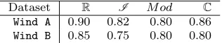
In this section we provide a more detailed long memory analysis of the complex-valued wind series described in Section 1.1. More specifically, we applied ourCLoMPE Hurst estimation method to the (detrended) irregularly sampled wind series to assess its persistence properties. The estimated Hurst parameter was ˆHC= 0.86 for the Wind Aseries and ˆHC= 0.8 for theWind Bseries, based onP = 50 lifting trajectories. Both of these estimates indicate moderate long memory.
To highlight potential differences with other approaches, we also performed the LoMPE technique
[image:14.595.338.496.576.607.2]of Knight et al (2017) to each of the real and imaginary components of the two series. In addition, we also esti-mated the Hurst exponent using the Knight et al (2017) method for the two magnitude series, since such se-ries (i.e. data without directional information) are most commonly analysed in the literature. The Hurst expo-nent estimates are denoted ˆHRand ˆHI for the real and imaginary component series, and ˆHM odfor the magni-tude series. The estimates are summarized in Table 3.
Table 3: Hurst parameter estimates for the Wind A and Wind B data from complex-valued series using CLoMPE and from real-valued component and mag-nitude series using LoMPE.
Dataset R I M od C
Wind A 0.90 0.82 0.80 0.86
Wind B 0.85 0.75 0.80 0.80
complex-0 20 40 60 80 100
0.0
0.2
0.4
0.6
0.8
1.0
Lag
A
CF
(a)
0 20 40 60 80 100
−0.2
0.0
0.2
0.4
0.6
0.8
1.0
Lag
A
CF
(b)
Fig. 4: (a) Autocorrelation for themagnitudewind series for theWind Aseries from Figure 1 (treated as regularly spaced); (b) autocorrelation for themagnitude Wind B dataset from Figure 1 (treated as regularly spaced). The dependence structure is markedly different to that shown for the real and imaginary series components shown in Figure 2.
valued structure of the data, thus accounting for its in-trinsic rotary structure and dependence, not visible by only using the traditional magnitude series or individ-ual real and imaginary strands.
It could also be argued that these differences in esti-mates are unsurprising, since the dependence structure for the magnitude series, shown in Figure 4, is visibly different to that of the real and imaginary component series shown in Figure 2. We argue that our estima-tion of the long memory parameter for this series is more reliable than that in the current existing litera-ture, as our proposed algorithm naturally encompasses both the complex-valued and improper features of wind series. A complex-valued analysis using our approach could hence provide more accurate long memory infor-mation, reducing miscalibration of predictive climate models. We further suggest that this precision would provide more certainty when assessing renewable en-ergy resource potential, as discussed in e.g. Bakker and van den Hurk (2012).
6 Discussion
Hurst exponent estimation is a recurrent topic in many scientific applications, with significant implications for modelling and data analysis. One important aspect of real-world datasets is that their collection and monitor-ing are often not straightforward, leadmonitor-ing to missmonitor-ing- missing-ness, or to the use of proxies with naturally irregular sampling structures. In parallel, in many applications
of interest there is a natural complex-valued represen-tation of data. To this end, this article has proposed the first Hurst estimation technique for complex-valued processes with sampling missingness or irregularity, and in doing so it has also constructed a novel lifting algo-rithm able to work on complex-valued data sampled with irregularity. Until the work in this article, Hurst estimation methods have not been able to exploit the wealth of signal information in such data, whilst also coping with irregular sampling regimes. OurCLoMPE wavelet lifting methodology was shown to give accurate Hurst estimation for a variety of complex-valued frac-tional processes, and is suitable for both proper and im-proper complex-valued processes. Simulations demon-strate that the technique is robust to estimation with significant degrees of missingness, as well as in the non-missing (regular) setting.
[image:15.595.62.511.103.287.2]Whilst the development of our proposed complex-valued Hurst estimator was motivated by an applica-tion in climatology, we believe that the work in this article has sufficient generality to have appeal in other settings. We thus conclude this article with outlining some example applications in which our methodology is potentially beneficial.
Data from neuroimaging studies. Functional mag-netic resonance imaging (fMRI) data continues to en-joy popularity in the neuroscience community due to its non-invasive acquisition and data richness, see e.g. As-ton and Kirch (2012) for an accessible introduction to the area from the statistical perspective. In particular, fMRI studies often measure information on blood flow in the brain; these voxel-level data are used to investi-gate neuronal activity of participants during task-based experiments, and many authors have asserted that such time courses possess fractional noise structure, see e.g. Bullmore et al (2003). Evaluation of the Hurst expo-nent in this context has been shown to be important in characterising brain activity under a range of condi-tions, indicating different levels of cognitive effort (Park et al, 2010; Ciuciu et al, 2012; Churchill et al, 2016). Despite data collection being performed in a controlled setup, recent work has highlighted the need for tailored statistical methodology to cope with both unbalanced designs, as well as missingness, which can feature in fMRI data for a number of reasons (Lindquist, 2008; Ferdowsi and Abolghasemi, 2017). In actuality, fMRI scanners record both phase and magnitude informa-tion, though most studies only use the magnitude image for analysis. As a result, there has been a recent body of work dedicated to complex-valued analysis of fMRI data, most notably by Rowe and collaborators (see e.g. Rowe (2005, 2009); Adrian et al (2017)). Such an ap-proach has shown improvements over real-valued meth-ods for a range of analysis tasks, see also the work by Adali and collaborators (Calhoun et al, 2002; Li et al, 2011; Rodriguez et al, 2012). Thus our methodology has the potential of taking advantage of the full complex-valued image information whilst also coping with the inherent non-uniform sampling.
Ocean surface measurement devices. There is a long-standing history of studying ocean circulation us-ing GPS-tracked ocean buoy drifters, see e.g. Osborne et al (1989). Since these trajectories are measured in the longitude-latitude plane, they are often converted to complex-valued vector series, see e.g. Sykulski et al (2017). It has long been observed that, due to the buf-feting motion of ocean currents, positional drifter tra-jectories often exhibit fBM-like behaviour, whilst their velocity over time resemble fGn characteristics (Sander-son and Booth, 1991; Summers, 2002; Qu and Addi(Sander-son,
2010; Lilly et al, 2017). In this context, accurate Hurst exponent estimation is useful in indicating the intensity of ocean turbulence, giving evidence towards particu-lar theorized dynamical regimes (Osborne et al, 1989). These in turn, can provide insight into initial conditions and origin of ocean circulation. Moreover, the trajec-tories often display rotary characteristics (Elipot and Lumpkin, 2008; Elipot et al, 2016). Due to the inter-rupted nature of satellite coverage and the possibility of measurements from multiple satellite orbits, the tem-poral sampling of the trajectories are typically highly nonuniform. In addition, due to the irregular sampling structure, the data are often interpolated prior to anal-ysis (Elipot et al, 2016). One aspect of exploration in this setting could be to contrast Hurst estimation using our proposed methodology with/ without data interpo-lation to investigate its effect, since previous work sub-stantiates that such processing can produce bias (in the context of Hurst exponent estimation) for real-valued series (Knight et al, 2017). It would also be interesting to investigate modifications to our technique to param-eter estimation for Mat´ern processes discussed in Lilly et al (2017).
Acknowledgements The R package CliftLRD implement-ing theCLoMPE technique will be released via CRAN in due
course.
A Proofs and theoretical results
This appendix gives the theoretical justification of the results from Sections 3 and 4, following the notation outlined in the text.
A.1 Proof of Proposition 1
To obtain the recursive construction for each basis, we start with the basis indexed byi= 1. At stagen, we havef(x) =
P
k∈Sncn,kϕ (1)
n,k(x) with ϕ
(1)
n,k(x) =χIn,k(x) as proposed in
the LOCAAT construction (Jansen et al, 2009). Let us now supposef(x) :=ϕ(1)n−1,j(x), thusϕ
(1)
n−1,j(x) =
d(1)jnψ (1)
jn (x) +
P
k∈Sn−1cn−1,kϕ (1)
n−1,k(x). Hence d
(1)
jn = 0, cn−1,k = 0,∀k=6 j andcn−1,j = 1. From the update
rela-tionshipcn−1,k=cn,k+bnkλjnfrom (7), we havecn−1,k= cn,k,∀k∈Jn(asλjn= 0 from d
(1)
jn = 0) and alsocn−1,k= cn,k,∀k /∈Jn.
From equations (5) we have
d(1)jn =λjn+iµjn=cn,jn ℓ
n jn+ im
n jn
+ X
k∈Jn
cn,k(ℓnk+ imnk).
(26)
By denoting an k = ℓ
n k+ im
n
k, we obtaind
(1)
jn = cn,jna
n jn−
P
k∈Jna
n
cn,jn=
an jn
|an jn|2
P
k∈Jna
n
kcn,k. Ifj∈Jnthencn,j = 1 and all
others are zero, socn,jn=
an jna
n j
|an jn|
2 := ˜anj. Thus
ϕ(1)n−1,j(x) =ϕ
(1)
n,j(x) + ˜a n jϕ
(1)
n,jn(x), ifj∈Jn, (27)
ϕ(1)n−1,j(x) =ϕ
(1)
n,j(x), ifj /∈Jn. (28)
For theprimal wavelet functionconstruction, we can similarly takef(x) :=ψ(1)jn (x), and obtain the corresponding wavelet
decomposition with coefficients d(1)jn = 1 (thus λjn = 1 and µjn = 0) andcn−1,k = 0,∀k6= jn. From the update
equa-tions, we havecn,j=−bnj,∀j∈Jnandcn,j= 0,∀j /∈Jn.
Usingd(1)jn = cn,jna
n jn−
P
j∈Jna
n
jcn,j (as above) and
d(1)jn = 1, we have cn,jna
n jn = 1−
P
j∈Jna
n
jbnj andcn,jn =
an jn
|an jn|2
1−P
j∈Jna
n jbnj
. Since f(x) := ψj(1)n (x), we then
have
ψj(1)n (x) = an
jn |an
jn| 2
1− X
j∈Jn anjb
n j
ϕ
(1)
n,jn(x)−
X
j∈Jn bnjϕ
(1)
n,j(x)
= a
n jn |an
jn| 2ϕ
(1)
n,jn(x)−
X
j∈Jn bn
j
ϕ(1)n,j(x) + ˜a n jϕ
(1)
n,jn(x)
.
Using the primal scaling function construction in equation (27), we obtain an expression for the primal wavelet function
ψj(1)n (x) = an
jn |an
jn| 2ϕ
(1)
n,jn(x)−
X
j∈Jn bn
jϕ
(1)
n−1,j(x),
which demonstrates the recursive construction from stagen ton−1 and concludes the proof for the primal wavelet and scaling function construction.
For thedualscaling functions, we use the update equa-tions and the fact thatcr,j=< f,ϕ˜r,j>for anyr, hence we
have, at stagen,
< f,ϕ˜n−1,j>=< f,ϕ˜n,j >+bnj < f,ψ˜ L
n,j>,∀j∈Jn
< f,ϕ˜n−1,j>=< f,ϕ˜n,j >∀j /∈Jn,
where ˜ψLdenotes the dual wavelet function corresponding to
theL-filter only.
Thus the recursive relations for the dual scaling functions are
˜
ϕn−1,j(x) = ˜ϕn,j(x) +bnjψ˜Ln,j(x),∀j∈Jn
˜
ϕn−1,j(x) = ˜ϕn,j(x),∀j /∈Jn.
Similarly, sinced(1)jn =cn,jna
n jn−
P
j∈Jna
n
jcn,j, we have
< f,ψ˜j(1)n >=< f, a
n jnϕ˜n,jn−
P
j∈Jna
n
jϕ˜n,j >and we obtain
the dual wavelet construction
˜ ψj(1)n =a
n
jnϕ˜n,jn(x)−
X
j∈Jn an
jϕ˜n,j(x).
These steps are subsequently re-iterated, and hence the same also holds for stager.
In order to obtain the primal scaling function recursive construction corresponding to the second basis, we proceed in the same way as for the first basis and similarly obtain
ϕ(2)n−1,j(x) =ϕ
(2)
n,j(x) + ˜a n jϕ
(2)
n,jn(x), ifj∈Jn,
ϕ(2)n−1,j(x) =ϕ
(2)
n,j(x), ifj /∈Jn.
We obtain the primal wavelet equations in a similar manner to the previous development
ψ(2)jn(x) = an
jn |an
jn| 2ϕ
(2)
n,jn(x)−
X
j∈Jn bn
jϕ
(2)
n−1,j(x).
The above equations show that the primal scaling and wavelet functions corresponding to the second basis are the conjugates of the corresponding primal and wavelet functions under the first basis, respectively.
As already explained, the update step is the same for both bases and cr,k =< f,ϕ˜(1)r,k >=< f,ϕ˜
(2)
r,k >, for all r, k thus
the dual scaling functions coincide under both bases ( ˜ϕ(1)r,k= ˜
ϕ(2)r,k).
For the dual wavelet function, following the same ap-proach as above, we obtain
˜
ψ(2)jn(x) =a
n
jnϕ˜n,jn(x)−
X
j∈Jn an
jϕ˜n,j(x).
This concludes the proof for the second basis.⊓⊔
A.2 Proof of Proposition 2
Let {Xt} be a zero-mean complex-valued stationary long
memory series with autocovariance γX(τ) ∼ cγ|τ|−β. We
note here that for improper processes of the type considered in Sykulski and Percival (2016), the pseudo-autocovariance has the same decay rate as the autocovariance (rX(τ)∼cr|τ|−β)
while for proper processes,rX(τ) = 0,∀τ, hence we shall
con-centrate on the lifting decorrelation properties for improper processes.
The autocovariance of {Xt} can be written as γX(ti−
tj) = E(XtiXtj) and rX(ti−tj) = E(XtiXtj), assuming
E(Xt) = 0, where 0 is to be understood as the complex
num-ber 0 = 0+i 0. Hence,E(d(ℓ)
j ) = 0 forℓ= 1,2. In what follows
we drop the superscript (ℓ) in order to avoid notational clut-ter.
Using the assumption thatE(dj) = 0 it follows that
E(dj
rdjk) =
Z
R ˜ ψjr(t)
Z
R ˜
ψjk(s)γX(t−s)ds
dt, (29)
where we have used djr =< X,ψ˜jr >, and the timepoints jr andjk are distinct. In what follows, denote the interval
length (i.e. continuous scale) of detaildjr byIr,jr.
Since from (15) and (22), regardless of whether we work with the basis indexed byℓ= 1 orℓ= 2, the (dual) wavelet functions are linear combinations of the (same) dual scaling functions, hence equation (29) can be re-written as
E(dj
rdjk) =
Z R ˜ ϕr,jr(t)−
X
i∈Jr Ar
iϕ˜r,i(t)
× Z R ˜
ϕk,jk(s)−
X
j∈Jk Ak
jϕ˜k,j(s)
γX(t−s)ds dt, (30)
whereA generically denotes the appropriate coefficient that corresponds to basis ℓ= 1 or ℓ= 2, but ˜ϕis the same for both bases.
As C2-LOCAAT progresses, the (dual) scaling functions