Article
Time-Dependent Probability Density Functions and
Attractor Structure in Self-Organised Shear Flows
Quentin Jacquet1,2 ID, Eun-jin Kim3,*ID and Rainer Hollerbach1 ID
1 Department of Applied Mathematics, University of Leeds, Leeds LS2 9JT, UK;
quentin.jacquet@ensta-paristech.fr (Q.J.); R.Hollerbach@leeds.ac.uk (R.H.)
2 ENSTA ParisTech Université Paris-Saclay, 828 Boulevard des Maréchaux, 91120 Palaiseau, France 3 School of Mathematics and Statistics, University of Sheffield, Sheffield S3 7RH, UK
* Correspondence: e.kim@sheffield.ac.uk; Tel.: +44-114-222-3876
Received: 30 July 2018; Accepted: 16 August 2018; Published: 17 August 2018
Abstract:We report the time-evolution of Probability Density Functions (PDFs) in a toy model of self-organised shear flows, where the formation of shear flows is induced by a finite memory time of a stochastic forcing, manifested by the emergence of a bimodal PDF with the two peaks representing non-zero mean values of a shear flow. Using theoretical analyses of limiting cases, as well as numerical solutions of the full Fokker–Planck equation, we present a thorough parameter study of PDFs for different values of the correlation time and amplitude of stochastic forcing. From time-dependent PDFs, we calculate the information length (L), which is the total number of statistically different states that a system passes through in time and utilise it to understand the information geometry associated with the formation of bimodal or unimodal PDFs. We identify the difference between the relaxation and build-up of the shear gradient in view of information change and discuss the total information length (L∞ = L(t → ∞)) which maps out the underlying attractor structures, highlighting a unique property ofL∞which depends on the trajectory/history of a PDF’s evolution.
Keywords: self-organisation; shear flows; coherent structures; turbulence; stochastic processes; Langevin equation; Fokker-Planck equation; information length
1. Introduction
Many systems in nature and laboratories are far from equilibrium, constantly changing in time and space and exhibiting very complex behaviour. Examples include turbulence in astrophysical and laboratory plasmas, the stock market, and biological ecosystems. Despite having apparently different manifestations of complexity, these systems have much in common and are often governed by similar nonlinear dynamics. In particular, an ‘ordered’ collective behaviour (e.g., in the form of coherent structures) emerges on the macroscale out of complexity as a novel consequence of self-organisation. For example, in the laboratory, in geophysical and astrophysical systems, coherent structures such as large-scale shear flows (such as zonal flows and streamers in laboratory plasmas, in the atmosphere and oceans, and in giant planets) and differential rotations in the Sun and other stars emerge from small-scale turbulence. There is overwhelming evidence from laboratory experiments, observations, and computational studies that these coherent structures play an absolutely critical role in determining the level of transport in the flow.
In particular, one crucial effect of shear flows is the suppression of transport in the direction orthogonal to the flow (the shear direction) by shear-induced enhanced dissipation [1–11]. This occurs as a shear flow distorts fluid eddies, accelerates the formation of small scales, and dissipates them when molecular diffusion becomes effective on small scales. This turbulence regulation leads to the formation of a transport barrier where transport is significantly reduced locally, providing one of
the crucial mechanisms for controlling the mixing and transport in a variety of systems. Important examples include (i) the low-to-high (L-H) transition (or internal transport barrier formation), during which a system undergoes a remarkable, spontaneous transition to a more ordered state, despite the increase in free energy (e.g., [3–5]); (ii) equatorial winds and polar vortices [12] (azimuthal flows in the east–west direction) which have long been known to reduce transport, acting as a transport barrier in the latitudinal direction [13]; (iii) transport barrier due to shear layers [14] in oceans which is called shear sheltering; and (iv) the solar tachocline—the boundary layer between the stable radiative interior and unstable convective layer which has a strong radial differential rotation—which can also act as a transport barrier, leading to weak anisotropic turbulence and mixing [5,7]. Our theoretical predictions of turbulent quenching in different systems have been confirmed by various numerical simulations (e.g., refs. [15,16]).
The foregoing statements underscore the importance of self-regulation between small-scale fluctuations and large-scale shear flows. We proposed a one-dimensional (1D) continuous model of self-organised shear flow [17] by extending a prototypical sand-pile model which evolves in discrete time. Specifically, we considered the formation of a shear flow driven by a short-correlated (white-noise) random forcing, where the shear gradient increases until it becomes unstable according to the stability criterion. For instance, in a strongly stratified medium, the stability is determined by the Richardson criterion: fluctuations on small scales (or internal gravity waves) amplify a shear gradient and thus, act as a forcing until the gradient exceeds the critical value given by the Richardson criterion, R= (A/N)2>Rc= (Ac/N)2=1/4. Here,Nis the buoyancy frequency due to the restoring force
(buoyancy) in a stably stratified medium, and Ais the shear gradient with the critical value Ac.
When unstable, the shear flow then relaxes its gradient and generates small-scale fluctuations, and this relaxation was modelled by nonlinear (cubic) diffusion; the shear gradient then grows again when small-scale turbulence becomes sufficiently strong to drive a shear flow. The same cycle repeats itself, exhibiting continuous growth and damping. This highlights that a self-organised state is never stationary in time, but involves persistent fluctuations.
The extension of refs. [17,18] solved a stochastic differential equation with a fourth-order stochastic Runga–Kutta method for Gaussian coloured noise in 1D and showed the transition from an unimodal stationary Probability Density Function (PDF) to a bimodal stationary PDF when the correlation time of a random forcing exceeds a critical value. The mean shear gradient is zero for a unimodal PDF, while its non-zero value represents the critical shear gradient around which a shear gradient continuously grows and damps through the interaction with fluctuations. The transition from a unimodal to bimodal PDF represents the formation of a non-zero mean shear gradient, or the formation of jets. Interestingly, In ref. [18], we found similar results in a 0D model and 2D hydrodynamic turbulence. In particular, the 2D results showed that a shear flow evolves through the competition between its growth and damping due to a localized instability, maintaining a stationary PDF, and that the bimodal PDF results from a self-organising shear flow with a linear profile.
length (L). While the detailed derivation ofLand its applications are given in refs. [22–32], it is useful to highlight thatLis a measure of the total elapsed time in units of a dynamical timescale for information change. To show this, we define the dynamical time (τ(t)) [22–30] as follows:
E ≡ 1
[τ(t)]2 =
Z 1
p(x,t)
∂p(x,t) ∂t
2
dx. (1)
Here,τ(t)is the characteristic timescale over which the information changes. Having units of time, τ(t)quantifies the correlation time of a PDF. Alternatively, 1/τquantifies the (average) rate of change of information in time.L(t)is then defined by measuring the total elapsed time (t) in units ofτas
L(t) =
Z t
0 dt1 τ(t1)
=
Z t
0
s
Z
dx 1
p(x,t1)
∂p(x,t1) ∂t1
2
dt1. (2)
L(t)measures the cumulative change inp(x,t), and depends on the intermediate states that a system evolves through between times 0 andt. Thus, it is a Lagrangian quantity (unlike entropy or relative entropy) which depends on the time history ofp(x,t), uniquely defined as a function of timetfor a given initial PDF.Lrepresents the total number of statistically distinguishable states that a system evolves through, providing a very convenient methodology for measuring the distance between p(x,t)andp(x, 0)continuously in time for a given p(x, 0). References [22–32] showed thatL∞is a new diagnostic for understanding a dynamical system and for mapping out an attractor structure. In particular,L∞captures the effect of different deterministic forces through the scaling ofL∞against the peak position of a narrow initial PDF. For a stable equilibrium, the minimum value ofL∞occurs at the equilibrium point. In comparison, in the case of a chaotic attractor,L∞exhibits a sensitive dependence on initial conditions like a Lyapunov exponent.
In this paper, we investigate the evolution of a shear gradient (x) starting from a relatively narrow PDF (p(x, 0)) with an initial mean value ofx0which represents the mean value of an initial shear
gradient. For a unimodal stationary PDF, the mean shear gradient decreases to zero in the long time limit, while for a bimodal stationary PDF with a peak of±x∗, the case ofx0>x∗models the relaxation
of an initial super-critical gradient (x0) to the critical value (x∗), and the case ofx0<x∗models the
build-up of the gradient from a subcritical initial value to the critical value (x∗). We are interested in the
information changes in these processes and in identifying the differences between the relaxation and build-up of the shear gradient in view of these information changes and in mapping out an attractor structure by usingL.
The remainder of this paper is organised as follows. We introduce our model and provide analytical solutions of time-dependent PDFs in limiting cases in Section2. In order to systematically undertake a numerical study, in Section3, we first provide a detailed discussion on stationary PDFs for different parameter values to determine the parameter space for unimodal versus bimodal PDFs. Section4provides numerical solutions for time-dependent PDFs andL. The discussion and conclusions are found in Section5.
2. Model
In this section, we introduce our model and provide analytical solutions for time-dependent PDFs in limiting cases. As noted in Section 1, given the universality of self-organisation in 0D, 1D, and 2D models and the challenge of the computation of time-dependent PDFs, we utilised a 0D model to facilitate the calculation of PDFs. Our 0D model is based on the cubic process for a stochastic variable (x) (e.g., representing a shear gradient). Specifically, we consideredxdriven by a finite correlated forcing (f), governed by the following Langevin equations
∂tx = −(ax+bx3) + f ≡ −g(x) +f, (3)
Here,g(x) =ax+bx3;a,b≥0 are constants;ξis a stochastic noise with a short correlation time with the correlation function
hξ(t)ξ(t0)i=2Dδ(t−t0). (5)
The highest cubic nonlinearity in our 0D model mimics a nonlinear cubic diffusion in the 1D model in refs. [17,18]. Equation (3) is the Ornstein–Uhlenbeck process [33] with the solution
f(t) = f(0)e−γt+
Z t
0 dt1e −γ(t−t1)
ξ(t1). (6)
For f(0) =0, the correlation time of f(t)is approximately 1/γ, as follows:
hf(t)f(t0)i=Rt 0dt1
Rt0
0 dt2e−γ(t−t1)e−γ(t 0−t
2)hξ(t
1)ξ(t2)i
= D
γ
h
e−γ(t0−t)−e−γ(t+t0)i≈ D γe
−γ|t0−t|, (7)
where we assumedt0 >tand used Equation (5). Thus,xin Equation (3) is driven by the Gaussian noise with the correlation timeγ−1. While the set of Equations (3) and (4) give a PDF in two dimensions
(x,f), it is useful to obtain an approximate PDF in thexdimension only. To this end, we combine Equations (3) and (4) to obtain the equation forxas
∂ttx+ (γ+∂xg)∂tx=−γg+ξ, (8)
and consider the overdamped limit where∂ttxis negligible compared with the damping term. This is
the so-called unified-colored noise approximation [34], and turns Equation (8) into
(γ+∂xg)∂tx ' −γg+ξ. (9)
We observe that for sufficiently smallγ, toO(γ)Equation (9) is, again, an Ornstein–Uhlenbeck process [33] forQ=g+γx:
∂tQ=−γQ+γ2x+ξ≈ −γQ+ξ. (10)
Thus, the mean value ofhQ(t)i=Q0e−γt, whereQ0=hQ(t=0)i, decays exponentially in time
while the variance,h(Q− hQi)2i= 21
β, evolves according to
1 2β =
e−2γt
2β0
+ D(1−e
−2γt)
γ , (11)
whereβandβ0=β(t=0)are the inverse temperatures ofp(Q,t)and its initial value, respectively. Therefore, the time-dependent PDF ofQis a Gaussian process and is given by
p(Q,t) =
r
β
πe
−β(Q−hQi)2
, (12)
whereβis the inverse temperature that satisfies Equation (11).
Since E in Equation (1) and L in Equation (2) are invariant under the change of variables, the Gaussian PDF ofQin Equation (12) provides us with a convenient way of calculating them by utilising the property of the Gaussian PDF. Specifically, for the Gaussian PDF ofQ,E is given by
E = (∂tβ)
2
2β2 +2β(∂thQi)
2, (13)
is dominated by the second term. Furthermore, with a smallD, Equation (11) becomes 2β∼2β0e2γt.
Thus, by substituting 2β∼2β0e2γt,∂thQi=−γQ0e−γtinto Equation (13), we obtain
E ∼2γ2β0Q20, (14)
where Q0 = (a+γ)x0+bx30, and x0 = hx(t = 0)iis the mean position of x att = 0. To relate
Equation (14) to what is observed in the PDF ofx, we need to find the initial inverse temperature, βx0 = 1/2h(x(0)−x0)2i, for p(x,t = 0)that corresponds toβ0 = 1/2h(Q(0)−Q0)2i(which is the
inverse temperature of the PDF ofQatt=0). To this end, we useQ− hQi= (a+γ)x+bx3− h(a+ γ)x+bx3i ∼(x− hxi)(a+γ+3bhxi2)to leading order for|hxi| |x− hxi|and obtain
h(Q− hQi)2i ∼ h(x− hxi)2i(a+γ+3bhxi2)2. (15)
Forx0γ,a, Equation (15) evaluated att=0 gives us
β0∼ βx0
9b2x4 0
. (16)
Equations (14) and (16) give us
E ∼ 2β
x 0γ2x20
9b2 , L(t)∼
r
2βx0
9b2 γx0t. (17)
Thus,L(t)increases linearly with time with a slope that is proportional toγandx0(for small
time, smallD, smallγ, and largex0). The numerical simulations in Section4examine this behaviour
in more detail.
Then, by using the conservation of the probability, the time-dependent PDF ofxis obtained as
p(x,t) =
dQ dx
p
(Q,t) =
r
β
π|∂xg+γ|exp
−β(Q− hQi)2
. (18)
It is interesting to note that p(x,t → ∞)in Equation (18) can be either unimodal or bimodal depending on the values of the parameters. This is discussed in detail in Section3.
Having gained some insight into the leading order behaviour ofp(x,t)for smallγ, we investigate a more general case of Equation (9). To this end, it is convenient to recast Equation (9) as
∂tx=− γg
G +
1
Gξ, (19)
whereG=∂xg+γ. The corresponding Fokker–Planck equation forp(x,t)is
∂
∂tp(x,t) = ∂
∂x
"
γg G p(x,t)
#
+D ∂
∂x
"
1 G
∂
∂x
1 Gp(x,t)
#
. (20)
3. Stationary PDFs
In order to undertake a systematic numerical study in Section4, we here provide a detailed discussion of stationary PDFs for different parameter values, and determine the parameter space for unimodal versus bimodal PDFs. A stationary PDF found from Equation (18) is
p(x)∝|G(x)| exp−γ D
Z x
g(x1)G(x1)dx1
=|∂xg+γ|exp
− γ
2D[g(x) 2+2
γ Z x
g(x1)dx1]
. (21)
ToO(γ), Equation (21) reproduces Equation (18). To determine the location of the local maxima and minima ofp(x)in Equation (21), we calculate
∂xp(x) =0 =⇒ − γ
D(∂xg+γ) 2g+
∂xxg=0. (22)
Forg=ax+bx3, Equation (22) can be rewritten as
xh−γ
D(a+γ+3bx
2)2(a+bx2) +6bi=0. (23)
Equation (23) gives the solutionx=0 andx6=0, indicating the possibility of the bimodal PDF. We then find the non-zero solution by solving
− γ
D(a+γ+3bx
2)2(a+bx2) +6b=0. (24)
To this end, it is convenient to make the following three successive changes in variables:
(
X=a+bx2, α= (Ω+3X)2X,
→
(
Y=1+3XΩ,
3α
Ω3 =Y2(Y−1),
→
(
Z=1/Y, Z3+δZ−δ=0,
(25)
withΩ,α,δdefined as
Ω=γ−2a, α= 6Db
γ , δ=
γ(γ−2a)3
18Db . (26)
In order to solve the equation forZin Equation (25), we use the Cardano formula and find the following three roots:
Z= 3 q δ
2(S+T), 3
q
δ
2(jS+j2T), 3
q
δ
2(j2S+jT).
(27)
Here,j=−1 2+i
q
3 2and
S= 3
s
1+
r
1+4δ
27, T=
3
s
1−
r
1+4δ
27. (28)
Equation (27) gives the non-zero solutions of Equation (24):
x2∗= 3
s
4D 3γb2Ψ−
γ+a
3b , (29)
where 1 Ψ =
S+T, jS+j2T, j2S+jT.
To find real solutions, we check the discriminant (∆) of the last equation of Equation (25),
∆=−27(−δ)2−4(δ)3=−4δ2
27 4 +δ
, (31)
as the sign of∆determines the number of the real root as follows:
• If∆<0, then one root is real, and two are complex conjugates,
• If∆=0, then all roots are real, and at least two are equal,
• If∆>0, then all roots are real and unequal.
From a detailed analysis of different cases provided in AppendixA, we conclude that the existence of a bimodal PDF requires∆ ≤0 in Equation (31), and that the peak position of a bimodal PDF is given by
x∗=±
v u u
t3
s
4D 3γb2
1 S+T −
γ+a
3b , (32)
where
δ= γ(γ−2a) 3
18Db , S=
3
s
1+
r
1+4δ
27, T=
3
s
1−
r
1+4δ
27.
Finally, a convenient method of identifying parameter values for unimodal versus bimodal PDFs is to check the sign of∂xxp(x)atx=0:
∂xxp
x=0
=h6b− γ
D(a+γ)
2ai. (33)
Since a unimodal PDF takes a local maximum atx=0 when∂xxp<0 and a local minimum at x =0 when∂xxp >0, we can see from Equation (33) that a unimodal PDF with∂xxp(x =0) <0 is
more likely for largerγand smallerD. Alternatively, a finite correlation time of f (smallγ) and a large diffusion (D) facilitate the formation of a bimodal PDF.
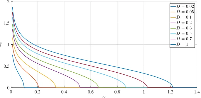
To illustrate these results, Figures1and2show how the peak positionx∗and peak amplitude p(x∗), respectively, vary withγfor a range ofDvalues. Figure3shows the boundary between the unimodal and bimodal PDFs in the{γ,D}parameter space. These results are fora=b=1, but other values yield the same general boundary shapes, and in particular, the same agreement occurs between the two different evaluation methods,R=0 and (33). The condition∂xxp(x=0)>0 is therefore a
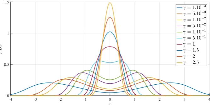
necessary and sufficient condition to have a bimodal PDF. Figure4shows what the PDFs look like and how the transition between unimodal and bimodal PDFs comes about.
0 0.2 0.4 0.6 0.8 1 1.2 1.4
γ 0
0.5 1 1.5 2
x∗
D= 0.02
D= 0.05
D= 0.1
D= 0.2
D= 0.3
D= 0.5
D= 0.7
[image:7.595.127.470.579.747.2]D= 1
0 0.2 0.4 0.6 0.8 1 1.2 1.4
γ
0.2 0.4 0.6 0.8 1 1.2 1.4 1.6 1.8
P
D
F
a
t
x∗
D= 0.02
D= 0.05
D= 0.1
D= 0.2
D= 0.3
D= 0.5
D= 0.7
[image:8.595.118.480.88.257.2]D= 1
Figure 2. The peak amplitudes (p(x∗)) as functions ofγ, for different values ofD, as indicated,
anda=b=1. The small diamonds indicate the transition points between unimodal and bimodal Probability Density Functions (PDFs).
0 0.2 0.4 0.6 0.8 1 1.2 1.4 1.6 1.8 2
γ 0
0.5 1 1.5 2 2.5 3
D
D solution of 3 q
4D
3γb2S+1T =γ+ a 3b D= γ
6b(a+γ)2a
Bimodal region
[image:8.595.130.468.320.490.2]U nimodal region
Figure 3. The boundary between unimodal and bimodal PDFs in the parameter space {γ,D}, fora=b=1. The red curve is the solution of∂xxp(x = 0) = 0, whereas the blue diamonds are
the result of settingR=0.
-4 -3 -2 -1 0 1 2 3 4
x
0 0.5 1 1.5
P
D
F
γ= 1.10−3 γ= 5.10−3 γ= 1.10−2 γ= 5.10−2 γ= 1.10−1 γ= 5.10−1 γ= 1 γ= 1.5 γ= 2 γ= 2.5
Figure 4.The stationary PDFs forD=0.7,a=b=1, andγ, as indicated. Note the transition between
unimodal PDFs for largeγand bimodal PDFs for smallγ, in agreement with the boundary shown
[image:8.595.131.466.552.720.2]4. Numerical Results
We provided analytical solutions for a time-dependent PDF in certain limiting cases, such as smallγ (e.g., Equation (12)), largex0and small time (e.g., Equation (17)) in Section2, and in the
limit of large time, where the PDF settles into a stationary solution, in Section3. To obtain exact time-dependent solutions to the Fokker–Planck equation (22) for any parameter values, we now use numerical methods in this section and utilise results from Section3to perform our numerical simulation systematically. As shown in AppendixB, we can seta= b=1 without any real loss of generality by rescaling the other quantities appropriately. The effective parameter space is therefore reduced to{γ,D}, together with whatever parameters define the initial condition, which we take to be p(x,t = 0) ∝ exp
−(x−x0)2/10−3
. That is, βx0 = 103 remains fixed, corresponding to a relatively narrow PDF, and the initial peak position (x0) is the one additional parameter. The initial
condition (p(x,t=0)) represents the PDF for an initial shear gradient. When the final stationary PDF is unimodal, the mean shear will decrease to zero in the long time limit; when the stationary PDF is bimodal with a peak of±x∗,x0 > x∗models the relaxation of an initial super-critical gradient (x0)
to the critical value (x∗) whilex0<x∗models the build-up of the gradient from an initial subcritical
value to the critical value (x∗). We are interested in the information change in this relaxation problem
and in identifying the difference between the relaxation and build-up of the shear gradient in view of the information change. The numerical implementation of Equation (22) is based on second-order accurate finite-differencing in bothxandt, with up to 104grid points inx, and timesteps as small as 10−4. The domain inxis truncated to the interval[−10, 10]rather than the original unbounded interval for which the analytic theory applies. As seen in Figure4, for example, for the parameter values of interest here, the PDFs are well-confined to the interval|x| ≤10, making a numerical solution of (22) with boundary conditions ofp=0 atx=±10 an excellent equivalent to an infinite interval.
4.1. Time Evolution of PDFs
Figure5shows examples of how different values ofx0ultimately all relax to the same final PDF.
Panels (a–d) correspond to x0 = 0, 0.32, 0.6, 1, respectively. γ = D = 1, according to Figure 3, is slightly in the bimodal regime, consistent with the final PDF seen here. Figure6focuses specifically on how the positions of the peaks evolve in time. Important observations that we can make from Figures5and6are as follows:
(a) An initial PDF with a peak atx0=0 remains unimodal before becoming a bimodal PDF;
(b) An initial PDF with a peak atx0=x∗(0.32 for this case) does not maintain the same peak position
atx∗, but moves outward first tox>x∗and then inwards tox∗. This initial outward movement
explains why the minimumL∞=L(t→∞)does not occur forx0=x∗in Section4.2;
(c) An initial PDF with a peak atx=xL(wherexLis thex0value which minimisesL∞, as defined
in Section4.2) constitutes the border line between different PDF evolutions (an initial PDF with a peak atx0<xLgoes outwards and then inwards, while an initial PDF with a peak atx0>xL
monotonically moves inwards tox∗);
Figure 5.Time evolution of the PDFs for the following initial conditions: (a)x0 =0; (b)x0 =0.32;
(c)x0=0.6; (d)x0=1.γ=D=1 for all four.
0 2 4 6 8 10 12 14 16 18
t
00.1 0.2 0.3 0.4 0.5 0.6 0.7 0.8 0.9 1
P
e
a
k
p
o
s
it
io
n
(a)
x
0= 0
(b)
x
0= 0
.
32
(c)
x
0= 0
.
6
(d)
x
0= 1
Figure 6.The peak positions of the solutions in Figure5as functions of time.
4.2. Information Length: Attractor Structure
[image:10.595.121.473.390.612.2]call itµ= dtdL(t), and compares with the analytic expectation
q
2βx0/9b2γx0in Equation (17). Thatµ is expected to scale linearly withγandx0and be independent ofD, is reasonably well reproduced by
the numerical data with less than a 10% difference between the theoretical prediction and simulation results (note the small range of they-axis).
20
10 12 14 16 18
8 6 4 2 0 t 0 10 20 30 40 50 60 70 80 L ( t ) 90
γ= 0.01, x0= 3 γ= 0.01, x0= 4 γ= 0.1, x0= 3 γ= 0.1, x0= 4 γ=1, x0=3 γ= 1, x0= 4
-1 0 1 2 3
-3 -4
-5 -2
log(t)
-8 -6 -4 -2 0 2 4 lo g ( L ( t ))
γ= 0.01, x0= 3
γ= 0.01, x0= 4
γ= 0.1,x0= 3
γ= 0.1,x0= 4
γ= 1, x0= 3
[image:11.595.92.492.156.279.2]γ= 1, x0= 4
Figure 7.L(t)as a function oft, with a linear scale on the left and a logarithmic scale on the right.
0.1 0.2 0.3 0.4 0.5 0.6 0.7 0.8 0.9 1
γ 55 56 57 58 59 60 61 62 µ / γ
D= 0.01
D= 0.05
D= 0.1
D= 0.5
D= 1
T heoretical curve
2 2.2 2.4 2.6 2.8 3 3.2 3.4 3.6 3.8 4
x0 6.7 6.8 6.9 7 7.1 7.2 7.3 7.4 7.5 7.6 µ /x 0
D= 0.01
D= 0.05
D= 0.1
D= 0.5
D= 1
T heoretical curve
Figure 8.Lettingµdenote the numerically computed slopeL(t)/t(for smallt), the left panel shows
µ/γas a function ofγ, forx0 =4, and the right panel showsµ/x0as a function ofx0forγ =0.5.
The agreement with the expectations from Equation (17) is seen to be reasonably good.
L∞(x0,D,γ) is a unique representation of the total number of statistically different states that a PDF evolves through to reach a final unimodal or bimodal PDF. The smaller L∞ is, the smaller the number of states that the initial PDF passes through to reach the final equilibrium. Therefore,L∞provides us with a path-dependent Lagrangian measure of the distance between a given initial and final PDF. Thus, by choosing a narrow initial PDF at different peak positions (x0), we can
map out the attractor structure (the proximity ofx0to an equilibrium) by measuringL∞as a function
ofx0. We were particularly interested in how differentlyL∞would behave for the final unimodal and
bimodal PDFs, which have different stable equilibrium points:x=0 andx=x∗6=0, respectively. To
this end, Figure9showsL∞as a function (x0) for a range ofDvalues. For final bimodal PDFs, the
location of the final peak position (x∗) is shown by a little vertical line.
We note first in Figure9that the overall shapes of the curves are drastically different depending on whether the final PDF is unimodal or bimodal. For a unimodal final PDF, the minimum value ofL∞ occurs forx0=0. This is becausex0=0 is a stable equilibrium for a unimodal PDF and thus, an initial
PDF with the peak (x0) closer tox=0 undergoes less change during the evolution of time and is more
similar to the final PDF. Therefore, the absolute minimum ofL∞occurs atxL =argminx0L∞(x0) =0,
[image:11.595.86.499.315.442.2]2
0 0.5 1 1.5
-0.5 -1
-1.5 -2
x0
2 4 6 8 10 12 14 16 18 20
L∞
(
x0
)
D= 0.01
D= 0.1
D= 0.5
D= 2
[image:12.595.107.490.85.278.2]Powered by TCPDF (www.tcpdf.org)
Figure 9.L∞as a function ofx0forD, as indicated, andγ=0.5.
In comparison,x = 0 is an unstable equilibrium point for a final bimodal PDF, whilex∗ 6= 0,
given by Equation (32), is a stable equilibrium point. Therefore,L∞ has a local maximum around x0=0 (unstable point). Naively, the minimum value ofL∞would be expected to occur for an initial
PDF withx0=x∗, that is, when the peak position of an initial PDF (x0) coincides with that of the final
PDF (x∗). However, the blue and green curves in Figure9reveal the very interesting fact thatL∞is actually minimised forx0=xL>x∗. As noted from Figures5and6, this is because the initial peaks
that are sufficiently far away move inwards monotonically, but the initial peaks nearx∗actually have a
more complicated evolution (moving outwards and then inwards).
These observations confirm thatL∞is a good Lagrangian measure that captures the attractor structure and dynamics. It is, thus, of particular interest to compareL∞with the Kullback–Leibler divergence [19] (that is commonly used in comparing PDFs), defined as
D(p||q) =
Z
p(x)ln
p(x)
q(x)
dx, (34)
wherep(x)is the initial PDF andq(x)is the final one. Obviously, unlikeL∞,D(p||q)depends only on the initial and final PDFs, and thus, does not provide any information on dynamics (e.g., what different states an initial PDF passes through in the time evolution, or how the locations and the shapes of the PDFs evolve in time between initial and final PDFs). Since we have an analytic expression for the stationary PDFs, we computedD(p||q)by numerical integration with the initial PDF used above. Figure10shows these results, where the little vertical lines represent the positions ofx∗.
We can see that the absolute minimum relative entropy always occurs whenx0 = 0 or x∗for
unimodal and bimodal PDFs, respectively, unlikeL∞. In retrospect, this is not particularly surprising, since the relative entropy only measures the difference between the two PDFs, and an initial PDF located at the final peak position is most similar to the final PDF. Specifically, for a bimodal PDF, the initial PDF at the peak position of the final PDF has the strongest resemblance to the final PDF, with the minimumD(p||q)occurring forx0=x∗.
For completeness, we also showD(q||p)in Figure11. Unlike Figure10, the absolute minimum value occurs atx0=0, even when the final PDF is bimodal, failing to capture the attractor structure
-2 -1.5 -1 -0.5 0 0.5 1 1.5 2
x
0-1 -0.5 0 0.5 1 1.5 2 2.5 3
D
(
p
||
q
)
D= 0.01
D= 0.1
D= 0.5
D= 2
[image:13.595.100.497.86.280.2]Powered by TCPDF (www.tcpdf.org) Powered by TCPDF (www.tcpdf.org) Powered by TCPDF (www.tcpdf.org)
Figure 10.Relative entropy (D(p||q)) as a function ofx0forD, as indicated, andγ=0.5.
-2.5 -2 -1.5 -1 -0.5 0 0.5 1 1.5 2 2.5
x0
100 101 102 103 104 105
D
(
q
||
p
)(lo
g
)
D= 0.01 D= 0.1 D= 0.5 D= 2
Figure 11.D(q||p)as a function ofx0forD, as indicated, andγ=0.5.
5. Discussion and Conclusions
We investigated the time evolution of PDFs in a toy model of self-organised shear flows using a unified coloured approximation, and utilised the information length to understand information changes and attractor structures. In our model, the formation of shear flows was induced by a finite memory time of a stochastic forcing and was manifested by the emergence of a bimodal PDF, with the two peaks representing non-zero mean values of a shear flow (gradient). We presented a thorough study of PDFs for different correlation time and amplitude values for the stochastic forcing. By solving the Fokker–Planck equation numerically, we investigated the time evolution of PDFs starting with a narrow PDF at different peak positions (x0) at timet=0. The cumulative change in information
(L∞) beautifully maps out the underlying attractor structures. Specifically, for a unimodal PDF, the minimum value ofL∞ occurs forx0 = 0, sincex0 = 0 is a stable equilibrium for a unimodal
PDF and thus, an initial PDF with a peak (x0) closer tox=0 undergoes less change during the time
evolution and is more similar to the final PDF; for a bimodal PDF,Lis minimised forx0=xL >x∗,
wherex∗is the peak position of a bimodal PDF. Recalling thatx0represents the mean shear gradient
[image:13.595.108.494.329.518.2]super-critical shear gradient is, in fact, more similar to a final stationary state, while an initial narrow PDF with a mean critical shear gradient undergoes a complicated evolution through the interaction with fluctuations. This is likely to be due to the rapid relaxation of instability at the super-critical state, similar to what was observed in the forward process in the phase transition in [27] (e.g., compare Figures6b and7b). That is, a process triggered by instability involves a smaller change in information and thus, a larger change in entropy (as might be expected as a consequence of instability). This reflects a unique property ofL∞which depends on a trajectory/history of a PDF evolution. In comparison, the relative entropy, which only measures the difference between the initial and final PDFs, does not provide any information on the dynamics between the initial and final times. In summary, we demonstrated the importance of studying the dynamics and the merit of the information length in understanding the dynamics and the evolution of PDFs in a toy model of self-organised shear flow. Further work will include the extension of this work to the analysis of our model without unified colored-noise approximation and to other turbulence models, in particular, to quantify the information change associated with intermittency and self-organisation.
Author Contributions: Original research idea, E.K.; Investigation, Q.J., E.K. and R.H.; Software, R.H.; Visualization, Q.J.; Supervision, E.K and R.H; Writing—original draft, E.K, Q.J. and R.H.; Writing—review and editing, E.K., Q.J. and R.H.
Funding:This research received no external funding.
Conflicts of Interest:The authors declare no conflict of interest.
Appendix A. Derivation of Equation (32)
Appendix A.1. Caseδ=−274 ⇐⇒ ∆=0
According to the definitions ofSandTin Equation (28),S=T=1. So, by using 1+j+j2=0,
we calculated Equation (30):
1 Ψ =
S+T=2,
jS+j2T=j+j2=−1, j2S+jT=j2+j=−1.
(A1)
Consistent with the statement above, we obtained three real solutions. The last two solutions with the same value of 1
Ψ =−1 in Equation (A1) make Equation (29):
x2∗=−
"
3
s
4D 3γb2+
γ+a 3b
#
<0, (A2)
which is inconsistent, sincex∗is a real number. On the other hand, the solutionΨ1 =S+T=2 can
give a consistent solution ifx2
∗in Equation (29) is positive, that is
R≡ 3
s
4D 3γb2
1 S+T−
γ+a
3b >0. (A3)
If not, the PDF is unimodal.
Appendix A.2. Caseδ>−274 ⇐⇒ ∆<0
∆<0 gives a unique real solution and two complex solutions which are complex conjugates. It is easy to see that the real solution of our interest corresponds to Ψ1 =S+Tbecause
q
1+4δ
27 is real.
Appendix A.3. Caseδ<−274 ⇐⇒ ∆>0
We can takeγ<2a, because ifγ>2a, thenδ>0 (see the last equation in Equation (26)). We thus take a root (Z∗) of the last equation of Equation (25) withδ<−274.
Appendix A.3.1. SubcaseZ∗ >0
Obviously, in this case,
Y∗= 1 Z∗
>0. (A4)
We recall that
X∗= γ−2a
3 (Y∗−1). (A5)
Usingγ−2a<0 and Equation (A4), we have
X∗ = 2a
−γ
3 (1−Y∗)< 2a−γ
3 < 2
3a, (A6)
which is in contradiction toX∗=a+bx20>a. Thus, there is no consistent non-zero solution in this case.
Appendix A.3.2. SubcaseZ∗ <0
Becauseδ<−274 <0,δZ∗>0. Using the last equation in Equation (25), we then have
Z3∗−δ=−δZ∗<0, (A7)
and thus,
Z3∗<δ< −27
4 ⇒Z∗<− 3
3
√
4. (A8)
Using Equation (A7) in Equation (A8) then gives us
Z3∗−δ=δ(−Z∗)< 27
4 Z∗<− 27
4 3
3
√
4. (A9)
Therefore,
Z3∗<δ−
27 4
3
3
√ 4 <−
27 4 (1+
3
3
√
4), (A10)
and
Y∗ = 1 Z∗ >−
1
3
q27
4(1+ √334)
. (A11)
So, using Equation (A11) in Equation (A5) gives us
X∗ = 2a
−γ
3 (1−Y∗)< 2a−γ
3
1+
1
3
q27
4(1+ √334)
<
2 3
1+
1
3
q27
4(1+ √334)
a'0.91a. (A12)
Equation (A12) is in contradiction with X∗ = a+bx2∗ > a. Therefore, there is no consistent
solution in this case. This proves that in the case∆>0, there is no consistent non-zero solution (x∗)
Appendix A.4. Summary
From the analyses above, we can conclude that the existence of a bimodal PDF requires∆≤0 and
R≡ 3
s
4D 3γb2
1 S+T−
γ+a
3b >0. (A13)
To make sure that this solution in Equation (29) corresponds to a local maximum, we need to show∂xxp(x=x∗)<0. To this end, we recall thatx∗satisfies Equation (23)
− γ
D(∂xg(x∗) +γ) 2g(x∗)
x∗ +6b=0. (A14)
We then find the second derivative of the stationary PDF atx∗, as follows:
∂xxp(x∗)exp
γ
2D
g(x∗)2+2γ Z x∗
g(x1)dx1
=
−2γ
D(∂xg+γ)g∂xxg
−γ
D(∂xg+γ) 2
∂xg+6b+
h
−γ
Dg∂xg
i h
−γ
D(∂xg+γ) 2g+
∂xxg
i
x=x∗
. (A15)
By using Equation (23), we see that the last term in Equation (A15) is identically zero. Furthermore, using Equation (A14), we simplify Equation (A15) as
∂xxp(x∗)exp
γ
2D
g(x∗)2+2γ Z x∗
g(x1)dx1
=hγ
D(∂xg+γ)
h
−2g∂xxg+ (∂xg+γ)(g
x−∂xg)
ii
|x=x∗
=−γ
D(a+γ+3bx 2 ∗)
h
12b(ax2∗+bx4∗) +2x2∗(a+γ+3bx2∗)
i
. (A16)
Since the exponential is positive,∂xxp(x∗)<0 in Equation (A16), confirming a local maximum of
a PDF atx=x∗.
Appendix B. Rescaling
We show, in detail, how we rescale Equations (3) and (4) to makea=b=1. We first rescalexby usingx=qabx˜in Equations (3) and (4) to recast them as
∂tx˜=
q b a h −a √ ax˜ √
b − a√√ax˜3
b +f
i
,
∂tf =−γf+ξ,
(A17)
and thus,
∂tx˜=−a(x˜+x˜3) +
q
b af, ∂tf =−γf+ξ.
(A18)
Next, we rescaletby usingt= a˜t
∂t˜x˜=−x˜−x˜3+1a
q
b af, ∂t˜f =−γaf+ξa.
We let ˜f = 1a
q
b af
∂t˜x˜=−x˜−x˜3+ f˜, ∂t˜f˜=−1aγf˜+a12
q
b aξ.
(A20)
We then let ˜γ= 1aγand ˜ξ= a12
q
b aξ
(
∂t˜x˜=−x˜−x˜3+f˜, ∂t˜f˜=−γ˜f˜+ξ˜.
(A21)
Finally, we rescalehξ˜(t)ξ˜(t0)i= ab5hξ(t)ξ(t0)i= ab5Dδ(t0−t) = ab4Dδ(t˜0−t˜) =D˜δ(t˜0−t˜).
References
1. Dam, M.; Brons, M.; Rasmussen, J.J.; Naulin, V.; Hesthaven, J.S. Identification of a predator-prey system from simulation data of a convection model.Phys. Plasmas2017,24, 022310. [CrossRef]
2. Chang, C.S.; Ku, S.; Tynan, G.R.; Hager, R.; Churchill, R.M.; Cziegler, I.; Greenwald, M.; Hubbard, A.E.; Hughes, J.W. Fast Low-to-High confinement mode bifurcation dynamics in a tokamak edge plasma gyrokinetic simulation.Phys. Rev. Lett.2017,118, 175001. [CrossRef] [PubMed]
3. Kim, E. Consistent theory of turbulent transport in two dimensional magnetohydrodynamics.Phys. Rev. Lett. 2006,96, 084504. [CrossRef] [PubMed]
4. Kim, E.; Dubrulle, B. Turbulent transport and equilibrium profile in 2D MHD with background shear.
Phys. Plasmas2001,8, 813. [CrossRef]
5. Kim, E. Self-consistent theory of turbulent transport in the solar tachocline I. Anisotropic turbulence.
Astron. Astrophys.2005,441, 763.
6. Leprovost, N.; Kim, E. Dynamo quenching due to shear. Phys. Rev. Lett. 2008,100, 144502. [CrossRef] [PubMed]
7. Kim, E.; Diamond, P.H. Zonal flows and transient dynamics of the L-H transition.Phys. Rev. Lett.2003,91, 075001. [CrossRef] [PubMed]
8. Li, J.; Kishimoto, Y. Numerical study of zonal flow dynamics and electron transport in electron temperature gradient driven turbulence.Phys. Plasmas2004,11, 1493. [CrossRef]
9. Idomura, Y.; Tokuda, S.; Kishimoto, Y. Global profile effects and structure formations in toroidal electron temperature gradient driven turbulence.Nucl. Fusion2005,45, 1571. [CrossRef]
10. Xu, G.S.; Wu, X.Q. Understanding L-H transition in tokamak fusion plasmas. Plasma Sci. Technol. 2017,
19, 033001. [CrossRef]
11. Itoh, K. Physics of zonal flows.Phys. Plasmas2006,13, 055502. [CrossRef]
12. Piani, C.; Norton, W.A.; Iwi, A.M.; Ray, E.A.; Elkins, J.W. Transport of ozone-depleted air on the breakup of the stratospheric polar vortex in spring/summer 2000.J. Geophys. Res. Atmos.2002,107, 8270. [CrossRef] 13. Shepherd, T.G. Rossby waves and two-dimensional turbulence in a large-scale zonal jet.J. Fluid Mech.1987,
183, 467. [CrossRef]
14. Hunt, J.C.R.; Durbin, P.A. Perturbed vortical layers and shear sheltering. Fluid Dyn. Res. 1999,23, 375. [CrossRef]
15. Sood, A.; Kim, E.; Hollerbach, R. Suppression of a laminar kinematic dynamo by a prescribed large-scale shear.J. Phys. A Math. Theor.2016,49, 425501. [CrossRef]
16. Newton, A.P.; Kim, E. A generic model for transport in turbulent shear flows.Phys. Plasmas2011,18, 052305. [CrossRef]
17. Kim, E.; Liu, H.; Anderson, J. Probability distribution function for self-organization of shear flows.
Phys. Plasmas2009,16, 052304. [CrossRef]
18. Newton, A.P.; Kim, E. On the self-organizing process of large scale shear flows.Phys. Plasmas2013,20, 092306. [CrossRef]
21. Wootters, W.K. Statistical distance and Hilbert space.Phys. Rev. D1981,23, 357. [CrossRef]
22. Nicholson, S.B.; Kim, E. Investigation of the statistical distance to reach stationary distributions.Phys. Lett. A 2015,379, 83–88. [CrossRef]
23. Nicholson, S.B.; Kim, E. Structures in sound: Analysis of classical music using the information length.
Entropy2016,18, 258. [CrossRef]
24. Heseltine, J.; Kim, E. Novel mapping in non-equilibrium stochastic processes.J. Phys. A2016,49, 175002. [CrossRef]
25. Kim, E.; Lee, U.; Heseltine, J.; Hollerbach, R. Geometric structure and geodesic in a solvable model of nonequilibrium process.Phys. Rev. E2016,93, 062127. [CrossRef] [PubMed]
26. Kim, E.; Hollerbach, R. Signature of nonlinear damping in geometric structure of a nonequilibrium process.
Phys. Rev. E2017,95, 022137. [CrossRef] [PubMed]
27. Hollerbach, R.; Kim, E. Information geometry of non-equilibrium processes in a bistable system with a cubic damping.Entropy2017,19, 268. [CrossRef]
28. Kim, E.; Tenkès, L.-M.; Hollerbach, R.; Radulescu, O. Far-from-equilibrium time evolution between two gamma distributions.Entropy2017,19, 511. [CrossRef]
29. Tenkès, L.-M.; Hollerbach, R.; Kim, E. Time-dependent probability density functions and information geometry in stochastic logistic and Gompertz models.J. Stat. Mech. Theor. Exp.2017,123201. [CrossRef] 30. Kim, E.; Lewis, P. Information length in quantum systems.J. Stat. Mech. Theor. Exp.2018,043106. [CrossRef] 31. Kim, E. Investigating information geometry in classical and quantum systems through information length.
Entropy2018,20, 574. [CrossRef]
32. Hollerbach, R.; Dimanche, D.; Kim, E. Information geometry of nonlinear stochastic systems.Entropy2018,
20, 550. [CrossRef]
33. Risken, H.The Fokker-Planck Equation: Methods of Solution and Applications; Springer: Berlin, Germany, 1996. 34. Jung, P.; Hanggi, P. Dynamical systems: A unified colored-noise approximation.Phys. Rev. A1987,35, 4464.
[CrossRef]
35. Klebaner, F.Introduction to Stochastic Calculus with Applications; Imperial College Press: London, UK, 2012. 36. Gardiner, C.Stochastic Methods, 4th ed.; Springer: Berlin, Germany, 2008.
37. Wong, E.; Zakai, M. On the convergence of ordinary integrals to stochastic integrals.Ann. Math. Stat.1960,
36, 1560. [CrossRef]
c