Model averaging in ecology: : a review of Bayesian, information-theoretic and tactical approaches for predictive inference

This is a repository copy of

Model averaging in ecology: : a review of Bayesian,

information-theoretic and tactical approaches for predictive inference

.

White Rose Research Online URL for this paper:

http://eprints.whiterose.ac.uk/127516/

Version: Accepted Version

Article:

Dormann, Carsten F., Calabrese, Justin M., Guillera-Arroita, Gurutzeta et al. (20 more

authors) (2018) Model averaging in ecology: : a review of Bayesian, information-theoretic

and tactical approaches for predictive inference. Ecological Monographs. pp. 485-504.

ISSN 0012-9615

https://doi.org/10.1002/ecm.1309

[email protected] https://eprints.whiterose.ac.uk/

Reuse

Items deposited in White Rose Research Online are protected by copyright, with all rights reserved unless indicated otherwise. They may be downloaded and/or printed for private study, or other acts as permitted by national copyright laws. The publisher or other rights holders may allow further reproduction and re-use of the full text version. This is indicated by the licence information on the White Rose Research Online record for the item.

Takedown

If you consider content in White Rose Research Online to be in breach of UK law, please notify us by

Model averaging in ecology: a review of Bayesian,

information-theoretic and tactical approaches

Carsten F. Dormann

, Justin M. Calabrese

, Gurutzeta Guillera-Arroita

,

Eleni Matechou

, Volker Bahn

, Kamil Barto ´n

, Colin M. Beale

, Simone

Ciuti

, Jane Elith

, Katharina Gerstner

, J´erˆome Guelat

, Petr Keil

, Jos´e

J. Lahoz-Monfort

, Laura J. Pollock

, Bj¨orn Reineking

, David R.

Roberts

, Boris Schr¨oder

, Wilfried Thuiller

, David I. Warton

, Brendan

A. Wintle

_{, Simon N. Wood}

_{, Rafael O. W¨uest}

_{& Florian Hartig}

1

_{Biometry and Environmental System Analysis, University of Freiburg,}

Germany

2

_{Smithsonian Conservation Biology Institute, Front Royal, USA}

3

_{School of BioSciences, University of Melbourne, Australia}

4

_{School of Mathematics, Statistics and Actuarial Science, University of Kent,}

UK

5

_{Department of Biological Sciences, Wright State University, USA}

6

_{Department of Wildlife Conservation, Institute of Nature Conservation}

PAS, Krak´ow, Poland

7

_{Department of Biology, University of York, UK}

8

_{Computational Landscape Ecology, Helmholtz Centre for Environmental}

Research-UFZ, Leipzig, Germany

_{iDIV, Leipzig, Germany}

10

_{Swiss Ornithological Institute, Sempach, Switzerland}

12

_{Univ. Grenoble Alpes, Laboratoire d’ ´Ecologie Alpine (LECA), CNRS,}

Grenoble, France

13

_{Univ. Grenoble Alpes, IRSTEA, UR EMGR, Grenoble, France}

14

_{Biogeographical Modelling, Bayreuth Center of Ecology and}

Geoecology, Technische Universit¨at Braunschweig, Germany

16

_{Berlin-Brandenburg Institute of Advanced Biodiversity Research (BBIB),}

Berlin, Germany

17

_{School of Mathematics and Statistics, Evolution & Ecology Research}

Centre, University of New South Wales, Australia

_{School of Mathematics, Bristol University, UK}

19

_{Group for Theoretical Ecology, University of Regensburg, Germany}

20

_{Laboratory of Wildlife Ecology and Behaviour, School of Biology and}

Environmental Science, University College Dublin, Ireland

December 6, 2017

Running head: Model averaging in ecology

Keywords: AIC-weights, ensemble, model combination, model averaging, nominal coverage, prediction averaging, uncertainty

Abstract 1

In ecology, the true causal structure for a given problem is often not known, and 2

several plausible models exist. It has been claimed that using weighted averages of 3

these models can reduce prediction error, as well as better reflect model selection 4

uncertainty. However, a large range of different model averaging methods exists, 5

raising the question of how they differ regarding these goals. A core question for an 6

analyst is thus to understand under which circumstances model averaging can improve 7

predictions and their uncertainty estimates. 8

Here we review the mathematical foundations of model averaging along with the 9

diversity of approaches available. The terms contributing to error in model-averaged 10

predictions are each model’s bias (i.e. the deviation of each model prediction from the 11

∗_{corresponding author; Tennenbacher Str. 4, 79106 Freiburg, Email: carsten.dormann@biom.}

unknown truth), variance of, and covariance among, model predictions, and 12

uncertainty of model weights. 13

If bias of contributing model predictions is substantially larger than their variance, 14

the advantage of reduced variance through weighted averages is greatly reduced. For 15

noisy data, which predominate in ecology, variance is probably often larger than bias 16

and model averaging becomes an option to reduce prediction error. Correlation 17

between model predictions also reduces the effect of model averaging, and to 18

counteract this effect, model weights could be adjusted to maximise the variance 19

reduction. 20

Model-averaging weights have to be estimated from the data, and this estimation 21

process carries some uncertainty, so that “optimised” model weights may not be better 22

than the use of arbitrary weights, such as equal weights for all models. In the presence 23

of inadequate models, however, estimating model weights is still likely to be superior 24

to equal weights. Many different methods to derive averaging weights exist, from 25

Bayesian over information-theoretical to optimised and resampling approaches, as 26

reviewed here. 27

We also investigate the coverage of the confidence interval of the prediction for 28

different ways to combine model prediction distributions, showing that they differ 29

greatly, and that the full model has very good coverage properties. Our overall 30

recommendations stress the importance of validation-based approaches and of 31

uncertainty quantification to avoid unreflected use of model averaging. 32

1

Introduction

33

Models are an integral part of ecological research, representing alternative, possibly 34

predictions about ecological systems (Mouquet et al., 2015). In many cases it is not 36

possible to clearly identify a single most-appropriate model. For instance, 37

process-based models may differ in the specific ways they represent ecological 38

mechanisms, but several different process models may accord with our ecological 39

understanding. Statistical models are limited in their complexity by the amount of data 40

available for fitting, making several combinations of predictors plausible, and different 41

modelling approaches are available for statistical analysis (e.g. Hastie et al., 2009; Kuhn 42

and Johnson, 2013). 43

Model averaging, as the weighted sum of predictions from several candidate 44

models, provides a potential avenue to avoid selecting a single model over others 45

similarly plausible. Scientists average model predictions for different reasons, most 46

prominently: (a) reducing prediction error through reduced variance, and partially by 47

(b) reducing prediction bias (based on arguments described in Madigan and Raftery, 48

1994), and (c) accommodating/quantifying uncertainty about model parametrisation 49

and structure (Wintle et al., 2003, see also section 2.3). 50

Here we focus on averaging sets of models that differ in structure, as opposed to 51

mere differences in initial conditions or parameter values (Gibbs, 1902; Johnson and 52

Bowler, 2009). The latter case in the statistical and physical literature is called 53

“ensemble”, while in ecology that term is used more loosely. For some ecological 54

examples of model averaging see Wintle et al. (2003); Thuiller (2004); Richards (2005); 55

Brook and Bradshaw (2006); Dormann et al. (2008); Diniz-Filho et al. (2009); Le Lay 56

et al. (2010); Garcia et al. (2012); Cariveau et al. (2013); Meller et al. (2014), and Lauzeral 57

et al. (2015). 58

Several previous publications have reviewed model averaging in ecology and 59

evolution, focussing exclusively on ‘information-theoretical model averaging’ 60

2011; Grueber et al., 2011; Nakagawa and Freckleton, 2011; Richards et al., 2011; 62

Symonds and Moussalli, 2011), probably under the influence of the AIC-weighted 63

averaging popularised by Burnham & Anderson (2002; Posada and Buckley 2004). 64

Bayesianmodel averaging has been treated less frequently in ecology (for an example 65

see Corani and Mignatti, 2015), but for an excellent recent review of this topic in the 66

context of Bayesian model selection see Hooten and Hobbs (2015, see also Hoeting et al. 67

1999; Ellison 2004; Link and Barker 2006). However, none of the above is a 68

comprehensive review of the state of knowledge across the available model averaging 69

approaches. 70

Our aim is to provide such a comprehensive review in the light of developments 71

over the last 20 or so years, summarising the actual mathematical reasoning and 72

offering an intuitive as well as technical entry, illustrated by case studies. We primarily 73

address averaging of predictions from correlative models, although most of the points 74

will similarly apply to mechanistic/process-based models (see, e.g., Knutti et al., 2010; 75

Diks and Vrugt, 2010, for a review in the context of climate and hydrological models, 76

respectively). We do not concentrate on averaging model parameters, because we agree 77

with the criticism summarised in Banner and Higgs (2017): parameters are estimated 78

conditional on the model structure; as the model structure changes, parameters may 79

become incommensurable (see Posada and Buckley, 2004; Cade, 2015; Banner and 80

Higgs, 2017, and Appendix S1 for short review of the parameter-averaging literature). 81

This review is divided into two parts: theoretical and practical. In the first we 82

present the mathematical logic behind model averaging, and why this alone puts 83

severe constraints onhowwe do model averaging. Then, in the second part, we review 84

the different ways model-averaging weights can be derived, comparing Bayesian, 85

information-theoretic and other tactical perspectives (i.e. those not derived from 86

of how to quantify model-averaged prediction uncertainty. We briefly illustrate model 88

averaging with two case studies, before closing with unresolved challenges and 89

recommendations. 90

2

The mathematics behind model averaging

91

Model averaging refers to the computation of a weighted-average predictionYe based 92

on the predictions of several (M) contributing models,Yb1,Yb2, . . . ,YbM: 93

e Y =

M X

m=1

wmYbm , with M X

m=1

wm= 1. (1)

Conceptually, the role of weightswmis to adjust predictions such that the average 94

prediction has improved properties over selecting a single among a number of 95

candidate models (for example, less bias, lower variance or closer-to-nominal coverage). 96

In accordance with virtually all applications of model averaging we encountered, we 97

first focus on how model averaging reduces prediction error, here quantified as mean 98

squared error (MSE) of a predictionYbmof modelm, which is composed of prediction 99

bias and prediction variance: 100

MSE(Ybm) = n

bias(Ybm) o2

+var(Ybm). (2)

We shall now decompose this equation to understand what contributes to prediction 101

error in the context of model averaging. 102

Bias, i.e. the difference between the prediction expectation and the truth (y∗_{), will}

103

depend directly on the bias of the contributing models, as well as their weights (eqn 1). 104

As the truth is unknown (except in simulations), the statistical model-averaging 105

literature typically makes the assumption that individual models have no bias (Bates 106

and Granger, 1969; Buckland et al., 1997; Burnham and Anderson, 2002). In contrast, 107

the focus of averaging process models is primarily on removing bias (e.g. Solomon 108

Prediction variance (arising fromnhypothetical repeated samplings) is composed

of two terms, the variance of each contributing model’s prediction,

var(Ybm) =

1 n−1

n X

i=1

(Ybm−Ybmi)2,

and the covariances between predictions of modelmandm′_:

cov(Ybm,Ybm′) =

1 n−1

n X

i=1

(Ybm−Ybmi)(Ybm′−Yb_mi′).

For the average of two predictions,Yb1andYb2, we have:

110

var(Ye) =w2₁var(Yb1) +w22var(Yb2) + 2w1w2cov(Yb1,Yb2). (3)

When averaging several models, we expand eqn (3) to: 111

var(Ye) = var  

M X

m=1

wmYbm  =

M X

m=1

w2_mvar(Ybm) + M X

m=1

X

m′_6=m

wmwm′cov(Yb_m,Yb_m′)

= M X m=1 M X

m′₌₁

wmwm′cov(Yb_m,Yb_m′) =

M X

m=1

M X

m′₌₁

wmwm′ρ_mm′var(Yb_m)var(Yb_m(4)′),

whereρmm′ is the correlation betweenYb_mandYb_m′.

112

Putting eqns 2 and 3 together we get: 113

MSE(Ye) =   M X m=1 wm

E(Ybm)−y∗   2 + M X m=1 M X n=1

wmwm′ρmnvar(Ybm)var(Ybm′),

(5)

whereE(Ybm)−y∗ =bias(Ybm)represents model misspecification bias. 114

2.1

Influences on the error of model-averaged prediction

Equation 5 allows us to make a number of statements about the potential benefits of 116

model averaging. Firstly, bias will typically remain unknown, as truthy∗ _{is unknown,}

117

but it can be estimated through (cross-)validation, and hence also the relative 118

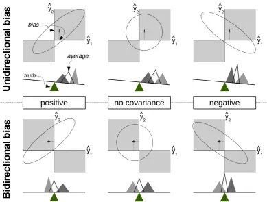
importance of bias to variability of predictions can be quantified (Fig. 1). When each 119

differences between models, then bias dominates (Fig. 1 top). As variance increases (or 121

bias decreases), the different model predictions overlap more and more, until bias is 122

small relative to variance (Fig. 1 bottom). Predictions from any model will now 123

typically have higher variance than the averaged prediction. Also, averaging can 124

reduce bias, if predictions scatter around the truth, but not unidirectional bias, that is if 125

all (most) model predictions err on the same side (see also Fig. 2 top row). However, if 126

predictions scatter around the truth, bias can be reduced by averaging. 127

[Fig. 1 approximately here.] 128

We thus conclude that as bias becomes large relative to prediction variance, model 129

averaging is less and less likely to be useful for reducing variance – it may still be 130

useful for reducing bias (under the condition of bidirectional bias: Fig. 2, lower row). 131

[Fig. 2 approximately here.] 132

Downweighting of variances is the mathematical reason how model averaging 133

reduces the variance over single model predictions. In the unlikely, but didactically 134

important case that predictions are independent, their covariance is 0 and the 135

correlation matrixρmnof eqn 5 becomes the identity matrix (or, equivalently, the 136

covariance term of eqn 4 vanishes). If we also assume both predictions have equal 137

variances (var(Yb1) =var(Yb2) =var(Yb)), and sincew2= 1−w1, the above equation

138

simplifies to var(Ye) = (2w2₁−2w1+ 1)var(Yb). If one model gets all the weight, we

139

have var(Ye) =var(Yb). If the two models receive equal weight, we have 140

var(Ye) = (2·(0.5)2−2·0.5 + 1)var(Yb) = 0.5var(Yb), a considerable improvement

141

in prediction variance (and the minimum of this equation). Other weights fall 142

in-between these values. More generally, Bates and Granger (1969) showed that for 143

unbiased models with uncorrelated predictions, the variance in the average is never 144

greater than the smaller of the individual predictions (making the important 145

words, model averaging can reduce prediction error because weights enter as quadratic 147

terms in eqn 3, rather than linearly. 148

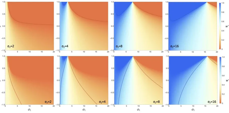
The correlation between model predictions, i.e. the matrix(ρij)∈RM×M, 149

substantially affects the benefit of model averaging (see also Fig. 3 and interactive tool 150

in the Appendix Data S2). In the best case, correlations between model predictions are 151

negative or at least absent, and the second term of eqn (5) is negative or vanishes. Here, 152

the variance in the average is dominated by individual models’ prediction variances. As 153

correlation between predictions increases, the covariance-term contributes more and 154

more to the overall prediction error, making the averaging of perfectly correlated 155

predictions exactly outweigh the benefit gained by the quadratic weights-effect for the 156

variances. 157

[Fig. 3 approximately here.] 158

This point provides some important insights about why some machine learning 159

methods that average a large number of bad models work so well. When averagingpoor

160

models, e.g. trees in a randomForest, covariance is negligible, but the variance of each 161

model prediction is high. Becausewmbecomes very small with hundreds of models 162

(around1/M), the variance of many averaged poor models (with similar variance) 163

tends to be low: var(Ye) =PM_{m=1 M}12var(Ybm) +_M12 PM

m=1

P

m6=ncov(Ybm,Ybn)≈ 164

M_M12var(Yb) = _M1 var(Yb),where the second term disappears due to lack of 165

correlations among predictions. We may speculate that poor models typically also 166

exhibit substantial but undirected bias, which again would be reduced by averaging. 167

The effect of correlations in the potential reduction of prediction error is rather 168

intuitive. If a prediction from a given model is extreme (e.g. on the high end of the 169

distribution), negative correlation will tend to balance out, while positive correlation 170

will accentuate total variance (e.g. Bohn et al., 2010). Ecologists know an analogous 171

(e.g. Thibaut and Connolly, 2013). It states that the fluctuation in biomass of a 173

community is less than the fluctuations of biomass of its members, because the species 174

respond to the environment differently. This asynchrony in response is analogous to 175

negative covariance in community members’ biomass, buffering thesumof their 176

biomasses. 177

Putting bias, variance and correlation together (Fig. 2), we note that model 178

averaging will deliver smaller prediction error when bias is “bidirectional” (i.e. model 179

predictions over- and underestimate the true value: bottom row of Fig. 2) and 180

predictions are negatively correlated (Fig. 2 bottom right). Uni-directional bias will 181

remain problematic (top row of Fig. 2), irrespective of covariances among predictions. 182

Thus, for a given set of weights, the prediction error of model-averaged predictions 183

depends on three things: the bias of the model average, the individual model prediction 184

variances, and the correlation between individual model predictions. 185

2.2

Estimating weights can thwart the benefit of model

averaging

Equation 5 assumes that the values of the weights are set a priori, and thus there is no 188

uncertainty about them. However, that would imply that an arbitrary set of weights is 189

used. Instead, the aim of optimising predictive performance suggests weights need to 190

be estimated from the data. But estimation brings associated uncertainty with it, and 191

this has implications for the actual benefits of model averaging: estimated “optimal” 192

weights will be suboptimal (Nguefack-Tsague, 2014), so the averaged prediction even 193

for only mildly correlated predictions will more likely be biased than if the (unknown) 194

truly optimal weights were used (Claeskens et al., 2016). It may in fact be often no 195

1989; Smith et al., 2009; Graefe et al., 2014, 2015). The “simple theoretical explanation” 197

provided by Claeskens et al. (2016) demonstrates that estimating weights introduces 198

additional variance into the prediction. As a consequence, the predictions averaged 199

with estimated weights may be worse than that of a single model (in contrast to the 200

assertion of Bates and Granger 1969; see Claeskens et al. 2016 for an example). 201

Finding optimal weights now becomes far more involved, and currently no closed 202

solution is available, not even for linear models (Liang et al., 2011). The interactive tool 203

we provide (Fig. 3) allows readers to explore this issue in a simple 2-model case. It 204

shows that, in this simple case, estimating weights substantially reduces the parameter 205

space where model averaging is superior to the best single model. 206

The performance reduction does not however imply that estimated weights are of 207

no use, or that the use of arbitrary weights (e.g. equal weights) is generally superior. 208

While uncertainty in estimated weights increases prediction error, the ability to 209

downweight or wholly remove unsuitable models from the prediction set is a 210

substantial benefit. In Claeskens et al. (2016) and similar simulations, all models 211

considered are “alright” (bias-free and with similar prediction variance), which 212

obviously need not be the case. Model weights are a measure of suitability for 213

prediction, which can be derived most logically from validation on (semi-)independent 214

data (see section 3 for details). If the unknown optimal model weights deviate strongly 215

from1/m, their estimation uncertainty is then a price worth paying. 216

2.3

Model averaging (typically) reduces prediction errors

The majority of studies we encountered (as random draws from the results of a 218

systematic literature search: see Appendix S7) used an empirical approach to assess 219

predictive performance, i.e. forecasting, hindcasting or cross-validation to observed 220

Montgomery et al., 2012; Smith et al., 2013; Engler et al., 2013; Edeling et al., 2014; 222

Trolle et al., 2014). Across the 180 studies we examined, model averaging generally 223

yielded lower prediction errors than the individual contributing models. Most of these 224

studies used test datasets to estimate predictive success, and rely critically on the 225

assumption of independence between test and training datasets (Roberts et al., 2017). 226

Few studies used simulated data to examine the performance of model averaging under 227

specific conditions (e.g. small sample size, model structure uncertainty, missing data: 228

Ghosh and Yuan, 2009; Schomaker, 2012). Very few studies provide mathematical 229

analyses (Shen and Huang, 2006; Potempski and Galmarini, 2009; Chen et al., 2012; 230

Zhang et al., 2013). 231

Summarising section 2 so far, we observe that 232

1. model averaging reduces prediction error by reducing prediction variance and 233

bias; 234

2. the more positively correlated predictions are, the smaller is the benefit gained 235

from averaging them; 236

3. when bias is large relative to the prediction variance of individual models, the 237

least-biased model will be a better choice than the model average; and 238

4. estimating weights introduces additional variance, outweighing, in some 239

situations, the benefits of model averaging. 240

2.4

Quantifying uncertainty of model-averaged

241

predictions

In random sampling, in addition to a statistic of interest, say a point prediction, we are 243

typically interested in the uncertainty of this statistic, e.g. as quantified by its variance 244

confidence intervals have nominal coverage, i.e. whether the true value is in the 95%-CI 246

indeed 95% of the time in repeated experiments. 247

If we attempt an analogy between random sampling and model averaging, the first 248

catch is that predictions from different models will be non-independent. In this case the 249

standard deviation does not decrease as square root ofn, but more slowly. The second 250

catch is that models are almost certainly not random draws from the population of 251

models (if we just think of all the models which we didnotinclude). Non-random 252

draws from a distribution are almost certain to yield biased estimates of that 253

distribution’s parameters. 254

The first catch can be taken care of by taking into account the variance-covariance 255

matrix of model predictions (see section 2, eqns 3-5). The second catch (models are 256

non-random draws) is harder and the severity of this problem depends on whether 257

model predictions are biased in the same direction (the “unidirectional bias” in Fig. 2) 258

or in different ways. Model averaging can only successfully unite diverging biased 259

predictions when they are biased in different directions. The approaches to computing 260

prediction variance below rely on the assumption that model predictions in fact do 261

scatter around the truth, and that the (weighted) average of model predictions is 262

unbiased. Since truth is unknown, this assumption cannot be tested. When models 263

share their fundamental structure (e.g. process models relying on the same equations), 264

it is more likely that they are unidirectionally biased. 265

2.4.1 Simplified error propagation in model-averaged predictions 266

To approximate the predictive variance of model-averaged predictions, Buckland et al. 267

2002, p. 159-162): 269

var(Ye) =  

M X

m=1

wm q

var(Ybm) +γ2m  

2

. (6)

Misspecification bias of modelmis computed asγm=Ybm−Ye, thus assuming 270

(explicitly on page 604 of Buckland et al. 1997) that the averaged point estimateYe is 271

unbiased and can hence be used to compute the bias of the individual predictions. This 272

assumption can be visualised in Fig. 2 as the situation where the empty triangles 273

always sit right on top of ‘truth’. This assumption is problematic as it cannot be met by 274

unidirectionally biased model predictions, nor when weightswmfail to get the 275

weightingexactlyright and thusYe remains biased. Less problematically, Buckland 276

et al. (1997) also assumed that predictions from different models areperfectly

277

correlated, making the covariance-term as large as possible, and variance estimation 278

conservative. The distribution theory behind this approach has been criticised as “not 279

(even approximately) correct” (Claeskens and Hjort, 2008, p. 207), but shown to work 280

well in simulations (Lukacs et al., 2010; Fletcher and Dillingham, 2011). 281

Improving on eqn (6) requires knowledge of the correlation matrixρmnof eqn (5). 282

The key problem is that there is no analytical way to compute the correlation of model 283

predictions. While bootstrapping models and their prediction can provide an estimate 284

ofρmn, it can more directly provide an estimate of var(Ye), rendering the indirect route 285

via eqn (6) unnecessary. 286

2.4.2 Coverage of the model-averaged prediction 287

Predictions from a selected single-best modelalwaysunderestimate the true prediction 288

error (e.g. Namata et al., 2008; Fletcher and Turek, 2012; Turek and Fletcher, 2012). The 289

reason is that the uncertainty about which model is correct is not included in this final 290

prediction: we predict as if we had not carried out model selection but had known from 291

Harrell, 2001). Thus, even if we were able to choose, from our model setM, the model 293

closest to truth, we would still need to adjust the confidence distribution for model 294

selection; however, a perfect adjustment was analytically shown not to exist (Kabaila 295

et al., 2015). 296

For statistical models, it is less clear whether the full model (i.e. prior to any model 297

selection; see Appendix S3) or model averaging computes the uncertainty intervals 298

correctly. Simulations suggest that model averaging may improve coverage (Namata 299

et al., 2008; Wintle et al., 2003; Zhao et al., 2013, none of who tested the full model), 300

which can be understood to happen because the process of averaging allows us to take 301

into account model uncertainty (Liang et al., 2011). Given that model averages need not 302

be normal (at the link scale), Fletcher and Turek (2012) and Turek and Fletcher (2012) 303

explore how to improve the tail areas of the confidence distribution, albeit under the 304

assumption that the true model is in the model set. Their approach was re-analysed by 305

Kabaila et al. (2015) under model selection. The key finding of this latter study is that 306

the full model coverage was still superior to all other model averaging approaches, 307

suggesting that the full model should currently be kept in mind, both for inference, 308

minimal bias and correct prediction intervals (see also Harrell, 2001, p. 59). Such 309

findings sit uncomfortably with the bias-variance trade-off (Hastie et al., 2009), which 310

states that overly complex models have poor predictive performance; and indeed the 311

full model has high prediction variance. However, our statements are about the 312

confidence intervals, rather than the point predictions, and those will be incorrectly 313

narrow for model selection without selection-correction. Regrettably, such reasoning 314

cannot be extended in an obvious way to models that do not have a “full model” 315

(non-nested models, process models, or machine learning models). Here model 316

averaging provides a way forward in representing prediction coverage more fairly. 317

section 3, these studies cannot be seen as conclusive, only as suggestive, for the 319

improvement of nominal coverage using model averaging. 320

In a different approach to characterising the uncertainty in model predictions, model 321

averaging can be interpreted as computing the distribution of a random variable that is 322

derived from a collection of random variables (the model predictions), also known as a 323

mixture distribution(Claeskens and Hjort, 2008, p. 217). In a two-step process, the 324

model weights determine the probability of choosing the model, and then the model 325

prediction is drawn from its confidence distribution. If predictions are unbiased, they 326

stack up high around the mean, and yield the same value as the equation for the 327

standard error of the mean. If predictions differ widely, e.g. due to bias, the mixed 328

confidence distribution will be much wider and possibly multi-modal. Mixing 329

distributions assumes their independence, i.e. the random draw of a value from one 330

model prediction is uncorrelated with the next draw of model and prediction. As model 331

predictions are likely to be positively correlated, assuming (conditional) independence 332

willunderestimatevariance (i.e. correlated draws would yield wider confidence 333

distributions). 334

Overall, this leaves us with the following options for computing the confidence 335

intervals of averaged predictions (which we will compute for a set of simple linear 336

regressions in Fig. 5): 337

1. Make the assumption that model-averaged predictions are unbiased (i.e. thaty∗ 338

can be estimated asYe). Use bootstrapping to estimate covariances of predictions 339

for each model. From these estimates, compute prediction variance according to 340

eqn (5). This solution is computer-intensive, but it takes into account covariance 341

of model predictions. (Note that simply averaging predictions from bootstrapped 342

2. Make again the assumption that model-averaged predictions are unbiased. Use 344

Buckland et al. (1997)’s approach (eqn 6). This will yield wider estimates than 345

option 1, because assuming perfect correlation is conservative. 346

3. Make the assumption that predictions from different models are effectively 347

uncorrelated. Use model mixing to compute the confidence distribution of the 348

average. 349

4. Fit the full model (if available) and use its confidence distribution, which can 350

rarely be improved on (Kabaila et al., 2015). 351

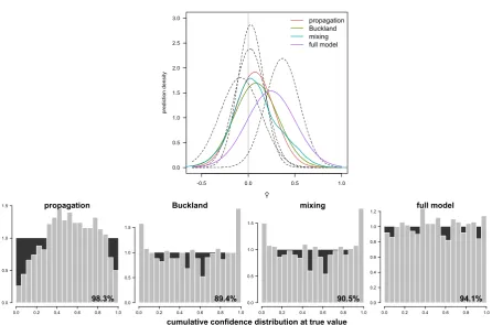
[Figure 5 approximately here.] 352

When averaging models with largely independent (i.e. uncorrelated) predictions, 353

only the bootstrap-estimated covariance matrix (option 1 above) will also compute 354

lower variances (according to eqn 4). In our illustration (Fig. 5, see Appendix S8), the 355

first three options (“propagation”, “Buckland” and “mixing”) hardly differ, while the full 356

model has a different location and is wider. The coverage of the 95% confidence 357

interval, computed through 1000 simulations, is best matched by the full model, while 358

the propagation approach is overly conservative. Buckland’s equation and mixing have 359

slightly too low coverage. 360

3

Approaches to estimating model-averaging

weights

When faced with predictions from very different models, estimating weights aims at 363

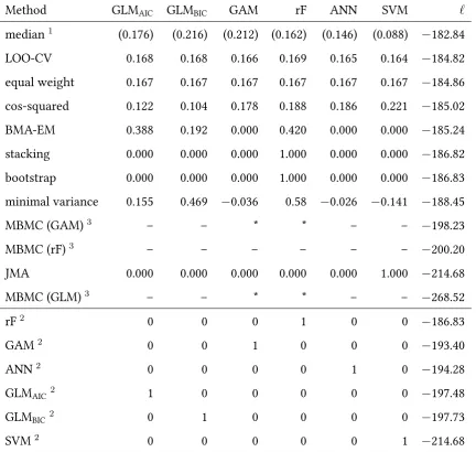
abating poorly, and elevating well predicting ones. For the resulting averaged 364

predictions, the actual method for estimating weights has obvious fundamental 365

elucidate on their interconnections (Table 1). Different perspectives on 367

model-averaging weights have emerged, which we present in somewhat arbitrary four 368

categories of decreasing probabilistic interpretability: 369

1. In the Bayesian perspective, model weights are probabilities that modelMiis the 370

‘true’ model (e.g. Link and Barker, 2006; Congdon, 2007). 371

2. In the information-theoretic framework, model weights are measures of how 372

closely the proposed models approximate the true model as measured by the 373

Kullback-Leibler divergence, relative to other models. 374

3. In a ‘tactical’ perspective, model weights are parameters to be chosen in such a 375

way as to achieve best predictive performance of the average. No specific 376

interpretation of the model is attached to the weights; they only have to work. 377

4. Assigning fixed, equal weights to all predictions can be seen as a reference na¨ıve 378

approach, representing the situation without adjusting for differences in models’ 379

predictive abilities. 380

We shall address these four perspectives in turn, also hinting at relationships 381

between them. 382

[Table 1 approximately here.] 383

3.1

Bayesian model weights

384

Our outline of Bayesian model weights follows that of Wasserman (2000), paying 385

attention to recent computational advances in the field. 386

Theory Bayes’ formula can be applied to models in much the same way as to 387

parameters. Hence, to perform inference with multiple models, one can write down the 388

joint posterior probabilityP(Mi,Θi|D)of modelMiwith parameter vectorsΘi, given 389

P(Mi,Θi|D)∝L(D|Mi,Θi)·p(Θi)·p(Mi), (7)

whereL(D|Mi,Θi)is the likelihood of modelMi,p(Θi)is the prior distribution of the 391

parameters of the respective modelMi, andp(Mi)is the prior weight on modelMi. 392

The joint distribution provides all information necessary for inference. Often, in 393

practice, we want to extract some simplified statistics from this distribution such as the 394

model with the highest posterior model probability, or the distribution of a parameter 395

or prediction including model selection uncertainty. To obtain this information, we can 396

marginalise (average, integrate) over parameter space, or marginalise over model space. 397

If we marginalise over parameter space, we obtain model weights (whilst 398

marginalising over model space yields averaged parameters, which we shall not 399

address here). The first step is to calculate the marginal likelihood, defined as the 400

average of eqn (7) across allkparameters for any given model: 401

P(D|Mi)∝ Z

Θ1

· · ·

Z

Θk

L(D|Mi,Θi)p(Θi)dΘ1· · ·dΘk (8)

From the marginal likelihood, we can compare models via theBayes factor, defined as 402

the ratio of their marginal likelihoods (e.g. Kass and Raftery, 1995): 403

BFi,j =

P(D|Mi)

P(D|Mj)

= R

L(D|Mi,Θi)p(Θi)dΘi R

L(D|Mj,Θj)p(Θj)dΘj

. (9)

with the multiple integral now pulled together for notational convenience. For more 404

than two models, however, it is more useful to standardise this quantity across all 405

models in question, calculating a Bayesian posterior model weightp(Mi|D)(including 406

model priorsp(Mi): Kass and Raftery, 1995, ) as 407

posterior model weight_i = p(Mi|D) =

P(D|Mi)p(Mi) P

jP(D|Mj)p(Mj)

(10)

Estimation in practice While the definition of Bayesian model weights and 408

challenging. In practice, there are two options to numerically estimate the quantities 410

defined above, both with caveats. 411

The first option is to sample directly from the joint posterior (eqn (7)) of the models 412

and the parameters. Basic algorithms such as rejection sampling can do that without 413

any modification (e.g. Toni et al., 2009), but they are inefficient for higher-dimensional 414

parameter spaces. More sophisticated algorithms such as MCMC and SMC (see Hartig 415

et al., 2011, for a basic review) require modifications to deal with the issue of different 416

number of parameters when changing between models. Such modifications (mostly the 417

reversible-jump MCMCs,rjMCMC: Green, 1995, see Appendix S5.1.1) are often 418

difficult to program, tune and generalise, which is the reason why they are typically 419

only applied in specialised, well-defined settings. The posterior model probabilities of 420

the rjMCMC are estimated as the proportion of time the algorithm spent with each 421

model, measured as the number of iterations the algorithm drew a particular model 422

divided by the total number of iterations. 423

The second option is to approximate the marginal likelihood in eqn (8) of each 424

model independently e.g. compute the maximum a posteriori model probability, 425

renormalise that into weights, and then average predictions based on these weights. 426

The challenge here is to get a stable approximation of the marginal likelihood, which 427

can be very problematic (Weinberg, 2012, see Appendix S5.1.2). Because of the 428

relatively simple implementation, this approach is a more common choice than 429

rjMCMC (e.g. Brandon and Wade, 2006). 430

Influence of priors A problem for the computation of model weights when 431

performing Bayesian inference across multiple models, is the influence of the choice of 432

parameter priors, especially “uninformative” ones (see section 5 in Hoeting et al., 1999; 433

The challenge arises because in eqns (8) and (9) the prior densityp(θi)enters the 435

marginal likelihood and hence the Bayes factor multiplicatively. This has the somewhat 436

unintuitive consequence that increasing the width of an uninformative parameter prior 437

will linearly decrease the model’s marginal likelihood (e.g. Link and Barker, 2006). 438

That Bayesian model weights are strongly dependent on the width of the prior choice 439

has sparked discussion of the appropriateness of this approach in situations with 440

uninformative priors. For example, in situations where multiple nested models are 441

compared, the width of the uninformative prior may completely determine the 442

complexity of models that are being selected. One suggestion that has been made is to 443

notperform multi-model inferenceat allwith uninformative priors, or that at least 444

additional corrections are necessary to apply Bayes factors weights (O’Hagan, 1995; 445

Berger and Pericchi, 1996). One such correction is to calibrate the model on a part of the 446

data first, use the result as new priors and then perform the analysis described above 447

(intrinsic Bayes factor: Berger and Pericchi 1996, fractional Bayes factor: O’Hagan 448

1995). If sufficient data are available so that the likelihood is sufficiently peaked 449

strongly during the calibration step, this approach should eliminate any complication 450

resulting from the prior choice (for an ecological example see van Oijen et al., 2013). 451

Bayesian variations In a set of influential publications, Raftery et al. (1997), 452

Hoeting et al. (1999) and Raftery et al. (2005) introducedpost-hocBayesian model 453

averaging, i.e. for vectors of predictions from already fitted models. The key idea is to 454

iteratively estimate the proportion of times a model would yield the highest likelihood 455

within the set of models (through expectation maximisation, see Appendix S5.2 for 456

details), and use this proportion as model weight. In the spirit of the inventors, we refer 457

to this approach asBayesian model averaging using Expectation-Maximisation 458

were not necessarily (and in none of their examples) fitted within the Bayesian 460

framework. It has been used regularly, often for process models (e.g. Gneiting et al., 461

2005; Zhang et al., 2009), where a rjMCMC-procedure would require substantial 462

programming work at little perceived benefit, but also in data-poor situations in the 463

political sciences (Montgomery et al., 2012). 464

Chickering and Heckerman (1997) investigate approximations of the marginal 465

likelihood in eqn (9), such as theBayesian Information Criterion(BIC, as defined 466

in the next section; see also Appendix S5.3) and find them to work well for model 467

selection, butnotfor model averaging. In contrast, Kass and Raftery (1995) state (on 468

p. 778) thateBIC_{is an acceptable approximation of the Bayes factor, and hence suitable}

469

for model averaging, despite being biased even for large sample sizes. These 470

approximations may be improved when using more complex versions of BIC (SPBIC 471

and IBIC: Bollen et al., 2012). 472

The “widely applicable information criterion”WAIC(Watanabe 2010 and an 473

equivalentWBIC: Watanabe 2013) are motivated and actually analytically derived in a 474

Bayesian framework (Gelman et al., 2014). Its uninformative prior implementation 475

should be seen as a variation of AIC (see next section), while the implementation with 476

model priors is based on posterior distribution of parameter estimates, and computed, 477

for each model, from two terms (Gelman et al., 2014): (1) the log pointwise predicted 478

density (lppd) across the posterior simulations for each of thenpredicted values, 479

defined as lppd= logQn_i=1pposterior(yi); and (2) a bias-correction term 480

pWAIC=Pni=1var(log(p(yi|θs))), where var is thesamplevariance over allSsamples

481

of the posterior distributions of parametersθ. Then the WAIC is defined as 482

WAIC=−2lppd+ 2pWAIC. In words, the WAIC is the likelihood of observing the data

483

under the posterior parameter distributions, corrected by a penalty of model 484

Model weights are computed from WAIC analogously to equation 11 below. 486

3.2

Information-theoretic model weights

487

In theinformation-theoreticperspective, models closer to the data, as measured by the 488

Kullback-Leibler divergence, should receive more weight than those further away. 489

There are several approximations of the KL-divergence, most famously Akaike’s 490

Information Criterion (AIC: Akaike, 1973; Burnham and Anderson, 2002). AIC and 491

related indices can be computed only for likelihood-based models with known number 492

of parameters (pm), restricting the information-theoretic approach to GLM-like models 493

(incl. GAM): 494

AICm=−2ℓm+ 2pm and wm =

e−0.5(AICm−AIC_min)

P

i∈Me−0.5(AICi−AICmin)

, (11)

whereℓmis the log-likelihood of modelm. 495

In the ecological literature, AIC (and its sample-size corrected version AICc, and its 496

adaptations to quasi-likelihood models such as QIC: Pan 2001; Claeskens and Hjort 497

2008) is by far the most common approach to determine model weights (for recent 498

examples see, e.g., Dwyer et al., 2014; Rovai et al., 2015).AIC-weights(eqn (11)) have 499

been interpreted as Bayesian model probabilities (Burnham and Anderson 2002, p. 75; 500

Link and Barker 2006), although we are not aware of a convincing theoretical 501

justification. An alternative interpretation is the proportion of times a model would be 502

chosen as the best model under repeated sampling (Hobbs and Hilborn, 2006), but such 503

an interpretation is contentious (Richards, 2005; Bolker, 2008; Claeskens and Hjort, 504

2008). In an anecdotal comparison, Burnham and Anderson (2002, p. 178) showed that 505

AIC-weights are substantially different frombootstrapped model weights. The 506

latter were proposed by Buckland et al. (1997) and represent the proportion of 507

simulations, AIC-weights did not reliably identify the model with the known lowest 509

KL-divergence or prediction error (Richards, 2005; Richards et al., 2011). Instead, 510

Mallows’ model averaging(MMA) has been shown to yield the lowest mean 511

squared error forlinearmodels (Hansen, 2007; Schomaker et al., 2010). Mallows’Cp 512

penalises model complexity equivalent to−2ℓm−n+ 2pm(forndata points; rather 513

than AIC’s−2ℓm+ 2pm, eqn 11). 514

Other approximations of the KL-divergence include Schwartz’ Bayesian 515

Information Criterion (see previous section), which was designed to find the most 516

probable model given the data (Schwartz, 1978; Shmueli, 2010), equivalent to having 517

the largest Bayes factor (see previous section).BICuseslog(n)rather than AIC’s “2” 518

as penalisation factor for model complexity (Appendix S5.3). A particularly noteworthy 519

modification of the AIC exist, where the model fit is assessed with respect to a focal 520

predictor value, e.g. a specific age or temperature range, yielding the Focussed 521

Information Criterion (FIC: Claeskens and Hjort 2008). We are not aware of a 522

systematic simulation study comparing the performance of these model averaging 523

weights, but AIC’s dominance should not indicate its superiority (see also case study 1 524

below). 525

The weighting procedure can additionally be wrapped into a cross-validation and 526

model pre-selection, which leads to the ARMS-procedure (Adaptive Regression by 527

Mixing with model Screening: Yang, 2001; Yuan and Yang, 2005; Yuan and Ghosh, 528

2008). We shall not present details on ARMS here (for cross-validation see next section), 529

because we regard model pre-selection as an unresolved issue (see section 5.3). 530

3.3

Tactical approaches to computing model weights

531

Methods covered in this section share the “tactical” goal of choosing weights to 532

explicitly building on Bayes or information theory thus most general in application. 534

Cross-validationapproximates a model’s predictive performance on new data by 535

predicting to a hold-out part of the data (typically between 5 and 20 folds). 536

Leave-one-out cross-validationdisturbs the data least, omitting each single data 537

point in turn. The fit to the hold-out can be quantified in different ways. If the data can 538

be reasonably well described by a specific distribution with log-likelihood functionℓ 539

(even if the model algorithm itself is non-parametric), the log-likelihood of the data in 540

thekfolds can be computed and summed (van der Laan et al., 2004; Wood, 2015, p. 36): 541

ℓm_CV =

k X

i=1

ℓ(y_[i]|θˆm_y

[−i_]), (12)

where the index[−i]indicates that the datay_[i]in foldiwere not used for fitting model

542

mand estimating model parametersθˆm

y[−i]. Cross-validation log-likelihood, specifically 543

leave-one-out cross-validation, is asymptotically equivalent to AIC and thus 544

KL-distance (Stone, 1977), albeit at a higher computational cost. The use of hold-out 545

data in cross-validation implicitly penalises overfitting, and we can hence compute 546

model weightswm

CVin the same way as AIC-weights (Hauenstein et al., 2017):

547

w_CVm = e

ℓm

CV

P i∈Meℓ

i

CV

. (13)

Other measures of model fit to the hold-out folds have been used, largely asad hoc

548

proxies for a likelihood function (e.g. in likelihood-free models): pseudo-R2(e.g 549

Nagelkerke, 1991; Nakagawa and Schielzeth, 2013), area under the ROC-curve (AUC: 550

Marmion et al., 2009a; Ordonez and Williams, 2013; Hannemann et al., 2015), or True 551

Skill Statistic (Diniz-Filho et al., 2009; Garcia et al., 2012; Engler et al., 2013; Meller 552

et al., 2014). In these cases, weights were computed by substitutingℓCVin eqn (13) by

553

the respective measure, or given a value of1/Sfor a somewhat arbitrarily defined 554

subset ofS(out ofM) models, e.g. those above an arbitrary threshold considered 555

Ordonez and Williams, 2013). 557

Largely ignored by the ecological literature are two other non-parametric

approaches to compute model weights:stackingandjackknife model averaging(see

Appendix S4 for discussion of averagingwithinmachine-learning algorithms). Both are

cross-validation based, and both optimise model weights on hold-out data.Stacking

(Wolpert, 1992; Smyth and Wolpert, 1998; Ting and Witten, 1999) finds the optimised

model weights to reduce prediction error (or maximise likelihood) on a test hold-out of

sizeH. This is, for RMSE and likelihood, respectively:

arg min wm        v u u u t 1 H H X i=1  y_[i]−

M X

m=1

wmfˆ

Xi θˆm

[−i]

 

2_

   

(Hastie et al., 2009) and

arg max wm     ℓ  y_[i]

M X m=1

wmfˆ

Xi θˆm

[−i]

      ,

wheref(Xˆ i|θˆm_[−i])is the prediction of modelm, fitted without using datai, to datai. 558

This procedure is repeated many times, each time yielding a vector of optimised model 559

weights,wm, which are then averaged across repetitions and rescaled to sum to 1. 560

Smyth and Wolpert (1998) and Clarke (2003) reports stacking to generally outperform 561

the cross-validation approach from two paragraphs earlier, and Bayesian model 562

averaging, respectively (see also the case studies in section 4 and Appendix S5). 563

InJackknife Model Averaging(JMA: Hansen and Racine, 2012), each data point 564

is omitted in turn from fitting and then predicted to (thus actually a leave-one-out 565

cross-validation rather than a “jackknife”). Then, weights are optimised so as to 566

minimise RMSE (or maximise likelihood) between the observed and the fitted value 567

across all “jackknife” samples. The optimisation function is the same as for stacking, 568

except thatH =N. Thus, in stacking, weights are optimised once for each run, while 569

for the jackknife only one optimisation over allN leave-one-out-cross-validations is 570

The forecasting (i.e. time-predictions) literature (reviewed in Armstrong, 2001; 572

Stock and Watson, 2001; Timmermann, 2006) offers two further approaches. Bates and 573

Granger (1969)’sminimal varianceapproach attributes more weight to models with 574

low-variance predictions. More precisely, it uses the inverse of the variance-covariance 575

matrix of predictions,Σ−1_{, to compute model weights. In the multi-model}

576

generalisation (Newbold and Granger, 1974) the weights-vectorwis calculated as: 577

wminimal variance = (1′Σ−11)−11Σ−1, (14)

where1_{is anM-length vector of ones. This is the analytical solution of eqn 5,}

578

assuming no bias and ignoring the problem that weights are random variates, under 579

the weights-sum-to-one constraint. Equation 14 does not ensure all-positive weights, 580

nor is it obvious how to estimateΣ_{. One option (used in our case studies) is to base}Σ

581

on the deviation from a prediction to test data in lieu of measure of past performance 582

(following recommendation of Bates and Granger, 1969). 583

Finally, Garthwaite and Mubwandarikwa (2010) devised a rarely used method, 584

called the “cos-squared weightingscheme”, designed to adjust for correlation in 585

predictions by different models. It was motivated by (i) giving lower weight to models 586

highly correlated with others (thereby reducing the prediction variance contributed 587

through covariances in eqn 5), (ii) division of weights when a new, near-identical 588

model prediction is added to the set, and (iii) reducing all weights when more models 589

are added to the set. Weights are computed as proportional to the amount of rotation 590

the predictions would require to make them orthogonal in prediction space, hence the 591

trigonometric name of their approach. 592

Model-based model combination: varying weights 593

Combining model predictions using statistical models, an approach we term 594

was first proposed by Granger and Ramanathan (1984). Here a statistical modelf is 596

used to combine the predictions from different models, as if they were predictors in a 597

regression:Ye ∼f(Yb1,Yb2, . . . ,Ybm)(see Fig. 4 left). The regression-type modelf can be 598

of any type, such as a linear model or a neural network. We call this regression the 599

“supra-model” in order to distinguish between different modelling levels. 600

A very simple supra-model would compute themedian of predictionsfor each 601

pointX_{i(e.g. Marmion et al., 2009a). Different models are used in the “average”}

602

without requiring any additional parameter estimation. Median predictions imply 603

varying weights, as the one or two models considered for computing the median may 604

change between differentX_i.

605

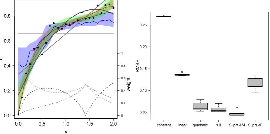
An ideal model combination could switch, or gently transition, between models 606

(such as manually constructed by Crisci et al., 2017). Since the predictions are combined 607

more or less freely in model-based model combinations to yield the best possible fit to 608

the observed data, MBMC should be superior to any constant-weight-per-model 609

approach (see Fig. 4 right), as was indeed found by Diks and Vrugt (2010). This 610

advantage comes with a severe drawback: a high proclivity to overfitting, as we fit the 611

same data twice (once to each model, then again to their prediction regression). 612

[Fig. 4 approximately here.] 613

This does not seem to be recognised as a problem (despite being a key message of 614

Hastie et al., 2009), as all studies we found incorrectly cross-validate the supra-model 615

only, not theentireworkflow (if at all; e.g. Krishnamurti et al., 1999; Thomson et al., 616

2006; Diks and Vrugt, 2010; Breiner et al., 2015; Romero et al., 2016). To correctly 617

cross-validate MBMCs, one has to produce hold-outsbeforefitting the contributing 618

models, and evaluate the MBMC prediction on this hold-out (Fig. 4, Appendix S5.9 and 619

case studies). 620

contributing models. As it is a yet fairly unexplored field in model averaging, analysts 622

are advised to try different supra-model types (Fig. 4). 623

3.4

Equal weights

624

In many fields of science (climate modelling, economics, political sciences), model 625

averaging proceeds with giving the structurally different models equal weight, i.e. 626

1/M (e.g. Johnson and Bowler, 2009; Knutti et al., 2010; Graefe et al., 2014; Rougier, 627

2016). In ecology, studies analysing species distributions reported equal weights to be a 628

very good choice when assessed using cross-validation (Crossman and Bass, 2008; 629

Marmion et al., 2009a; Rapacciuolo et al., 2012), but no better than the single models on 630

validation with independent data (Crimmins et al., 2013). Equal weights may serve as a 631

reference approach to see whether estimating weights reduces prediction error for this 632

specific set of models. In that sense, we may argue, all the above weight estimation 633

approaches only serve to separate the wheat from the chaff; once a set of reasonable 634

models has been identified, equal weights are apparently a good approach. 635

4

Case studies

All methods discussed above can be applied to simple regression models, while some 637

explicitly rely on a model’s likelihood and can thus not be used for non-parametric 638

approaches. We therefore devised two case studies, the first being a rather simple 639

example to illustrate the use of all methods in Table 1, and the second a more 640

complicated species distribution case study based on a reduced set of methods. Note 641

that we do not include adaptive regression by mixing with model screening (ARMS: 642

Yang, 2001) because its more sophisticated variations (Yuan and Yang, 2005) are not 643

preselected set of models. 645

4.1

Case study 1: Simulation with Gaussian response,

many models and few data points

In this first, simulation-based case study, we explore the variability of model-averaging 648

approaches in the common case where several partially nested models are fit (see 649

Appendix S9 for details and code). The simulation was set up so that several of the 650

fitted models have similar support as explanations for the data. This was achieved by 651

generating the response differently in each of two groups (using similar, but not 652

identical predictors). We simulated 70 data points with 4 predictors yielding24 = 16 653

candidate models, and another 70 for validation. We computed model weights in 19 654

different ways (Table 1) and compared the prediction error of weighted averages as 655

well as the individual models to the validation data points. Simulation and analyses 656

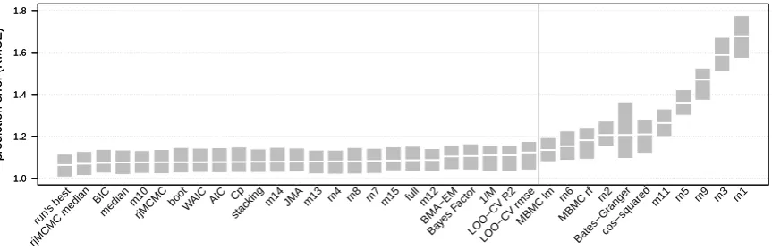
were repeated 100 times. 657

Two results emerged from this simulation that are worth reporting. First, 658

prediction error (quantified as RMSE) was similar across the 19 weight-computing 659

approaches, with a few noticeable exceptions, and most were no better than those of 660

the best nine single model predictions (the two MBMC approaches, minimal variance 661

and the cos-squared scheme: Fig. 6). Second, most averaging approaches gave some 662

weight (w >0.01) to ten or more models (Table 2), despite models being overlapping 663

and partially nested, so that we have actually only five (more or less) independent 664

models (those containing only one predictor: m2, m3, m5, m9 and intercept-only m1). 665

In real data sets, such spreading of weight is the result of data sparseness or extreme 666

noise, making important effects stand out less; indeed, half of our candidate models are 667

[Figure 6 approximately here.] 669

[Table 2 approximately here.] 670

4.2

Case study 2: Real species presence-absence data,

many data points and a moderate number of predictors

In the second case study we use data on the real distribution of short-finned eel 673

(Anguilla australis) in New Zealand (from Elith et al., 2008). The data are provided in 674

the R-package dismo, already split into a 1000-rows training and a 500-rows test data 675

set, and featuring 10 predictors. We ran four different model types (GAM, 676

randomForest-rF, artificial neural network-ANN, support vector machine-SVM), along 677

with two variations of the GLM (best models selected by AIC and BIC). For details see 678

Appendix S10. 679

The number of averaging approaches that can be used to compute model weights is 680

smaller than in the previous case study, as three of the six models do not report a 681

likelihood or the number of parameters, precluding the use of rjMCMC, Bayes factor, 682

(W)AIC, BIC, and Mallows’ Cp. In addition, because we do not know the underlying 683

data-generating model, we evaluate the models on the randomly pre-selected test data 684

provided. 685

[Table 3 approximately here.] 686

One interesting result is that model averaging was effectively a model selection tool 687

in several cases (Table 3). Stacking, bootstrapping, JMA, and to a lesser degree minimal 688

variance, BMA-EM and the model-based model combinations yielded non-zero weights 689

for only 1 (or 2) models. Apparently, these approaches yielded sub-optimal model 690

weights, as these “model selection”-outcomes of model averaging fared worse than 691

Secondly, the best two model averaging algorithms in this case study, apart from 693

the median where varying weights are used, identified an approximately equal 694

weighting as optimal strategy. That is somewhat surprising, given that SVM performed 695

relatively poorly (and was excluded by BMA-EM, but favoured by cos-squared as a 696

more independent contribution). The likely reason of high weights for the poor SVM is 697

that averaging-in less correlated predictions reduces covariances in eqn (5). 698

The good performance of the median in both case studies suggests that using the 699

central value ofeach prediction, rather than give constant weights to the model itself, 700

may be even more effective in reducing variance and thus prediction error. 701

5

Recommendations

702

Despite setting out to review the field of model averaging for ecologists, the complexity 703

of the topic prevents us from providing final answers. The recent mathematical 704

explanation why estimating optimal weights makes the averaged predictions perform 705

poorly (Claeskens et al., 2016) is an example for fundamental limitations of model 706

averaging. Many issues seem to be statistically unresolved, or addressed by quick-fixes 707

and even fundamental questions remain open, which we will discuss in the final 708

section. 709

It is unsatisfactory to see the large variance in weights and performance of the 710

different averaging approaches in our case studies. Also the literature provides too few 711

comparisons of model weights to provide robust advice. In general, our 712

recommendations are thus guided by reducing harm, rather than suggesting an optimal 713

5.1

Averaged prediction should be accompanied by

uncertainty estimates

Just like any other statistical approach, model averaging can also be misapplied. 717

Focussing entirely on the predictions rather than their spread can mislead, as Knutti 718

et al. (2010) showed for combining precipitation predictions: spatial heterogeneity 719

cancelled out across models, giving the erroneous impression of little change when in 720

fact all models predict large changes (albeit in different regions). Similarly, King et al. 721

(2008) found that averaging parameters from two competing models led to no effect of 722

two hypothesised impacts, although in both models a (different) driver was very 723

influential. We thus strongly encourage including at least model-averaged confidence 724

intervals alongside any prediction, possibly in addition to the individual model 725

predictions, to prevent erroneous interpretation of averaged predictions. Also, more 726

attention should be paid to the full model. It has many desirable properties (unbiased 727

parameter estimates, very good coverage), but suffers from violation of the parsimony 728

principle (“Occam’s razor”) and requires more consideration in which form covariates 729

should be fit. Its larger prediction error, compared to the over-optimistic single-best 730

partial model, is the reason for correct confidence intervals. 731

5.2

Dependencies among model predictions should be

732

addressed

Statistical models, which aim to describe the data to which they are fitted, will often 734

have correlated parameters and fits; process models may overlap in modelled processes. 735

Having highly similar models in the model set will inflate the cumulative weight given 736

to them (as illustrated in Appendix S6) . One way to handle inflation of weights by 737

Another approach would be to pre-select models of different types (see next point). 739

Alternatively, the cos-square scheme of Garthwaite and Mubwandarikwa (2010) uses 740

the correlation matrix of model projections to appropriately change weights of 741

correlated models. It is the only approach currently doing so, and, while the jury is still 742

out on this method, our case study results look only mildly promising (Fig. 6, Tables 2 743

and 3). 744

5.3

Validation-based weighting or validation-based

pre-selection of models

Madigan and Raftery (1994), Draper (1995) and more recently Yuan and Yang (2005) 747

and Ghosh and Yuan (2009), have argued that only “good” models should be averaged. 748

Different ways of combining model averaging with a model screening step have been 749

proposed (Augustin et al., 2005; Yuan and Yang, 2005; Ghosh and Yuan, 2009), in which , 750

model selection precedes averaging (pre-selection). This will happen implicitly, and in 751

a single step, if any of the model weight algorithms discussed above attributes a weight 752

of effectively zero to a model, as happened in case study 2. How prevalent this effect is 753

in real world studies is unclear, as weights are rarely reported. 754

In contrast, some studies select modelsafterthe predictions are made (e.g. Thuiller, 755

2004; Forester et al., 2013). These studies have averaged models which predict in the 756

same direction (along the “consensus axis”: Grenouillet et al. 2010), which are the best 757

50% in the set (Marmion et al., 2009a), or however many one should combine to 758

minimise prediction error. Such approaches necessitate addressing the challenge of 759

using data twice (Lauzeral et al., 2015). Post-selection reduces the ability of “dissenting 760

voices” (i.e. less correlated predictions) to reduce prediction error and instead reinforce 761

uncertainty estimation will be overly optimistic. We do not advocate their use. 763

We suggest to employvalidation-based methods of model averagingrather 764

than relying on model-based estimates of error, i.e. (leave-one out) cross-validation and 765

stacking rather than AIC. On account of us rarely believing our models in ecology, test 766

data give us some capacity to make allowances for predictive bias. It is probably of 767

little practical relevance whether models are pre-selected by validation-based estimates 768

of error and then averaged with equal weights or weighted by validation-based 769

estimates of error without pre-selection. 770

5.4

Process models are no different

In fishery science, averaging process models is relatively common (Brodziak and Piner, 772

2010), as it is in weather and climate science (Krishnamurti et al., 1999; Knutti et al., 773

2010; Bauer et al., 2015). There are at least two connected challenges such enterprises 774

face: validation and weighting. Often process models are tuned/calibrated on all sets of 775

data available, in the logical attempt to describe all relevant processes in the best 776

possible way. That means, however, that no independent validation data are available, 777

so that we cannot use the prediction accuracy of different models to compute model 778

weights. Consequently, all models receive the same weight (e.g. in IPCC reports, or for 779

economic models), or some reasonable but statistically ad-hoc construction of weights 780

is employed (e.g. Giorgi and Mearns, 2002). In recent years, hind-casting has gained in 781

popularity, i.e. evaluating models by predicting to past data. This will only be a useful 782

approach if historic data were not used already to derive or tune model parameters, 783

and if hindcasting success is related to prediction success (which it need not be, if 784

processes or drivers change). 785

Cross-validation is often infeasible for large models, as run-times are prohibitively 786