A Genetic Algorithm Approach for Optimising Traffic Control Signals Considering Routing

This is a repository copy of A Genetic Algorithm Approach for Optimising Traffic Control Signals Considering Routing.

White Rose Research Online URL for this paper: http://eprints.whiterose.ac.uk/84765/

Version: Accepted Version

Article:

Teklu, F, Sumalee, A and Watling, DP (2007) A Genetic Algorithm Approach for Optimising Traffic Control Signals Considering Routing. Computer-Aided Civil and Infrastructure Engineering, 22 (1). 31 - 43. ISSN 1093-9687

https://doi.org/10.1111/j.1467-8667.2006.00468.x

(c)2007 Computer-Aided Civil and Infrastructure Engineering. Published by Blackwell Publishing. This is an author produced version of a paper published in Computer-Aided Civil and Infrastructure Engineering. Uploaded in accordance with the publisher's self-archiving policy.

[email protected] https://eprints.whiterose.ac.uk/ Reuse

Items deposited in White Rose Research Online are protected by copyright, with all rights reserved unless indicated otherwise. They may be downloaded and/or printed for private study, or other acts as permitted by national copyright laws. The publisher or other rights holders may allow further reproduction and re-use of the full text version. This is indicated by the licence information on the White Rose Research Online record for the item.

Takedown

If you consider content in White Rose Research Online to be in breach of UK law, please notify us by

A Genetic Algorithm Approach for

Optimising Traffic Control Signals Considering Routing

Fitsum Teklu Research Student

Institute for Transport Studies University of Leeds

38 University Road, Leeds, LS2 9JT, United Kingdom Tel: +44 113 343 1788

Fax: +44 113 343 5334 Email: [email protected]

Agachai Sumalee

Senior Research Fellow, PhD Institute for Transport Studies University of Leeds

38 University Road, Leeds, LS2 9JT, United Kingdom Tel: +44 113 343 5345

Fax: +44 113 343 5334

Email: [email protected]

David Watling*

Professor, PhD

Institute for Transport Studies University of Leeds

38 University Road, Leeds, LS2 9JT, United Kingdom Tel: +44 113 343 6612

Fax: +44 113 343 5334

Email: [email protected]

A Genetic Algorithm Approach for

Optimising Traffic Control Signals Considering Routing

F. Teklu, A. Sumalee, and D. Watling

Institute for Transport Studies, University of Leeds

Abstract

It is well-known that co-ordinated, area-wide traffic signal control provides great potential for

improvements in delays, safety and environmental measures. However, an aspect of this

problem that is commonly neglected in practice is the potentially confounding effect of

drivers re-routing in response to changes in travel times on competing routes, brought about

by the changes to the signal timings. This paper considers the problem of optimising signal

green and cycle timings over an urban network, in such a way that the optimisation anticipates

the impact on traffic routing patterns. This is achieved by including a network equilibrium

model as a constraint to the optimisation. A Genetic Algorithm (GA) is devised for solving

the resulting problem, using total travel time across the network as an illustrative fitness

function, and with a widely-used traffic simulation-assignment model providing the

equilibrium flows. The procedure is applied to a case-study of the city of Chester in the UK,

and the performance of the algorithms is analysed with respect to the parameters of the GA

method. The results show a better performance of the signal-timing as optimised by the GA

method as compared to the other method which does not consider re-routing. This

improvement is found to be more significant with a more congested network whereas under a

relatively mild congestion situation the improvement is not very clear.

1 Introduction

In an urban transportation network, traffic signals have been used to control vehicle

movements so as to reduce congestion, improve safety, and enable specific strategies such as

1997). Through the years, procedures for determining optimum signal timings have been

developed and continuously improved. Early methods such as that of Webster (1958) only

considered a single signalised junction in isolation. Later, fixed time strategies were

developed that optimised a group of signalised junctions using historical flow data (e.g.

TRANSYT: Robertson, 1969). In some cities, real time traffic flow data has also been used

for optimisation in methods commonly referred to as demand-responsive strategies (e.g.

SCOOT: Hunt et. al., 1981). The focus of this research is on fixed time signal plans.

As mentioned earlier, fixed time plans use historical flows observed on links (through traffic

counts) to optimise signal timings. One shortcoming of such optimisation procedures is the

assumption that the flows for which the optimal timings are calculated will remain unchanged

after the new timings are implemented. This may not be a valid assumption if the

implementation of such timings substantially improves the journey time on a certain route,

since the users of alternative routes may divert to the improved route as a result. Such effects

have been observed as a consequence of area wide traffic control schemes (e.g. Almond and

Lott, 1968).

From a modelling viewpoint, the impact of signal time changes on changes in link flows

could also be explained from the perspective of traffic assignment theory. In a transportation

network, where traffic signals are explicitly modelled, drivers’ route choices in a network

could be assumed to a follow Wardrop User Equilibrium (UE) condition (Wardrop, 1952).

From such a perspective, a change in traffic signal timings will cause a change in the

equilibrium route choice behaviour of drivers through the link and route travel times, thus

altering the equilibrium link flow pattern over the network. Such an equilibrium model may

problem), to reflect the anticipated impact of changes to the timings on the flow patterns – i.e.

the flows are determined endogenously, inside the optimisation process.

Such a problem of determining optimum signal timings while anticipating the equilibrium

response of drivers is an instance of the Network Design Problem, NDP. A NDP is concerned

with improving an existing network so that some total network measure is optimised with

respect to some discrete or continuous design variables, while considering users’ response to

the improvement. Some examples of NDPs include the capacity enhancement problem

(Abdulaal and LeBlanc, 1979), the signal-setting problem (Chiou, 1999; Ceylan and Bell,

2004), toll pricing (Shepherd and Sumalee, 2004) and the charging cordon design problem

(Sumalee, 2004).

NDPs are characterized by the so called bi-level structure. On the upper level, a transport

planner is assumed to ‘design the network’, by selecting values for the design parameters so

as to optimise some measure of total social cost (e.g. total delay, pollution, social welfare).

Road users respond to that design in the lower level by altering their travel choices so as to

minimise their own travel costs, which may not agree with the planner’s view of the most

appropriate costs*. Formally, the planner’s optimisation in the upper level is constrained by

the lower level equilibrium problem. Such problems are known to be one of the most

challenging mathematical problems in the optimisation field, due to the non-smoothness of

the objective function (not differentiable everywhere), coupled with the non-convexity of the

feasible region. These properties imply the potential existence of multiple optima, as well as

great difficulty in devising robust and efficient methods for even finding local optima (see,

Luo et al, 1996 for more details).

*

A wide range of solution methods have been applied in an attempt to devise an efficient

technique to solve NDPs, ranging over heuristic iterative methods (Steenbrink, 1974; Allsop,

1974; Suwansirikul et al, 1987), linearization methods (LeBlanc and Boyce, 1986); Ben-Ayed

et al, 1988), sensitivity-based methods (Friesz et al, 1990; Yang, 1997), Karush-Kuhn-Tucker

based methods (Marcotte, 1986; Verhoef, 2002), methods developed from the system optimal

solution (Dantzig et al. 1979; Marcotte, 1981; Bergendorff et al, 1997; Hearn and Ramana,

1998), marginal function method (Meng et al, 2001), cutting plane method (Lawphongpanich

and Hearn, 2004), and stochastic search methods (Friesz et al, 1992; Cree et al, 1998; Ceylan

and Bell, 2004).

This paper presents a solution method for solving a signal timing based NDP using a

metaheuristic optimisation method, namely a Genetic Algorithm (GA). GA is an evolutionary

optimization technique, formulated on the basis of the mechanics of natural selection and

evolution. It offers great flexibility in solving such optimization problems as it does not

require any information on the gradient of the objective function and has the ability to move

out of local optima. An additional motivation for using GA for this problem is the simulation

based framework (as opposed to an analytic one) commonly employed in signal setting

methods (e.g. TRANSYT and SATURN) that do not use explicit mathematical relations

which negates the use of derivative based optimisation methods. GA has been used widely in

the transportation field, for problems such as generating zoning (Balling et al, 2004) or

activity plans (Charypar and Nagel, 2005), transit network design (Bielli et al, 2002;

Chakroborty, 2003), transit scheduling (Chakroborty et al, 1998), traffic parameter estimation

(Sharma et al, 2004), dynamic traffic management (Lo et al, 2001; Abu-Lebdeh and

In signal timing design, GA has been used to optimise cycle time, green time, offsets, and

stage sequences (e.g. Foy et al., 1992; Park et al., 2000; Park and Yun, 2005). These

applications, however, are limited to problems in which no account is taken of re-routing in

the optimisation, andwith the possible exception of Park and Yun who consider a twelve

intersection networkare limited to small networks with few signalised intersections. In the

network design context, Lee (1998), Taale and Van Zuylen (2003) and Ceylan and Bell

(2004) used GA in optimising signal timings, while anticipatingre-routing impacts. For stage

length and cycle time optimisation (without considering offsets) to minimize total travel time,

Lee (1998) presented a comparison of GA and simulated annealing with iterative and local

search algorithms and showed the different algorithms perform better for different network

supply and demand scenarios. Van Zuylen and Taale (2003) reported promising results from

applying a GA to optimise green times within a NDP context, albeit on small artificial

networks. In their approach to the NDP, Ceylan and Bell (2004) used the inverse of a system

performance index, defined as the weighed sum of delays and stops for all traffic streams in

the network, to optimise a common cycle time, green times and offsets. Flows were

constrained to a Stochastic User Equilibrium solution (Daganzo and Sheffi, 1977). Using a

small network, they showed that a bi-level framework with GA gives more efficient results

than an iterative algorithm in terms of system-wide travel costs. Although with a different

application in mind, GA has also been proposed for addressing a number of problems with a

similar bi-level structure, such as the analyses of Kim et al (2001) and Stathopoulos and

Tsekeris (2004) on the equilibrium-based OD matrix estimation problem; and those of Yin

(2000) and Sumalee (2004) on bi-level NDPs.

Building on Ceylan and Bell’s work we aim in the current paper to present a GA based signal

timings optimisation method that considers drivers rerouting and its application on a large

method that does not consider rerouting. The impact of the choice of GA parameters on the

performance of the algorithm is also presented. An illustrative objective function of total

network-wide travel time will be adopted, though clearly many alternative objectives could be

incorporated. . A simulation-assignment model provides the junction delays based on which

travel costs are calculated. Besides delays at signalised junctions, the model also enables the

consideration of delays at non-signalised junctions.

The next section presents the problem formulation and defines signal control design

parameters. The methodology description is given in section 3. The performance of the

program is analysed in Section 4, with conclusions given in the final section.

2 The Problem of Optimising Signals with Equilibrium Constraints

The NDP of optimising signal timings while anticipating drivers’ re-routing is defined in the

present section, and is hereafter referred to as ‘The Problem’.

2.1 Problem Formulation

The Problem is formulated as a Mathematical Program with Equilibrium Constraints (MPEC).

The planner’s upper level objective of minimizing total travel time† (TT) by altering signal

timings is constrained so that the associated flows are at User Equilibrium based on the travel

times resulting from the given signal timings. Additional signal setting feasibility constraints

are also applied. The notation used is given in TABLE 1.

[INSERT TABLE 1 HERE]

TT is defined as the sum of the product of the link flows and travel times over the whole

network. At junctions each turning movement is represented by a separate link of zero-length,

which has the associated delay put as travel time and included in the calculation of TT. TT is

influenced by the signal timings,, and link flow pattern q*( ) in the network; see Section

2.2.

Mathematically the problem is defined as:





a

t

q

q

q

TT

Min

))

(

,

(

))

(

,

(









 (1)

subject to: (C,,)o (2)

i. e. C_min CC_max (3)

0_h  C 1 (4)

max , , min

,r hr hr

h  

   (5)

h I C h h S r r h S r r

h  







and subject to the constraint that for a given  , the UE flow vectorq*( ) is given by the

variational inequality (Smith, 1979),

( , *) ( *) 0

t  q  q q   q (7)

where t and q are the vectors of travel time function and link flow respectively; and  is the

feasible space of the link flow vector.

In this paper, the traffic equilibrium problem is solved by use of the simulation-assignment

modelling software package SATURN (Van Vliet, 1982). In contrast to conventional traffic

assignnment models, SATURN places great emphasis on the detailed representation

intersections, turning movements, and associated junction conflicts. Based on the principles of

cyclic flow profiles (Robertson, 1969), its simulation sub-model determines junction delays at

a number of flow states, based on junction turning demands estimated by the assignment

sub-model. It uses this information to estimate marginal relationships between the travel time on

each link/turn and the flow on that link/turn, and these functions are then passed back to the

‘diagonalisation’ algorithm. The assignment sub-model uses the well-known Frank-Wolfe

convex combinations method to determine the equilibrium flow pattern. Although for given

travel-time/flow functions the assignment sub-model has guaranteed convergence to an

equilibrium solution, the process by which the assignment and simulation sub-models are

alternately solved is a heuristic one. Nevertheless, the widespread use of this heuristic in

practice has provided strong numerical evidence that good convergence can be assured

through experimentation with the heuristic process.

2.2 Signal timing design variables and feasibility constraints

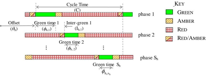
For a junction, FIGURE 1 shows the signal design variables: cycle time, offset, and the green

time for the different stages. A phase is the set of movements which can take place

simultaneously or the sequence of signal indicators received by such movements. The portion

of the cycle over which a given combination of phases is given green is called a stage. For all

signalised junctions, the offset – the difference in time of the start of the green between

adjacent junctions – is defined from a common reference time for one (randomly chosen)

stage. At a junction, the start of the green times for successive stages is defined by the

inter-green period, measured from the end of the inter-green of the preceding stage. For the problem

formulated in Section 2.1, the technical feasibility of the design variables, which is ensured by

equations (3) to (6), is explained briefly in the following paragraphs.

[INSERT FIGURE 1 HERE]

To maintain signal coordination from cycle to cycle each junction in the area considered must

operate with a common cycle time or a simple multiple of it (IHT, 1997). The common

network cycle time,C , is constrained to a minimum,C_min, and a maximum,C_max, as shown in

accommodate the inter-green times and the minimum green times as shown in (8). In the

numerical tests reported later,C_maxis constrained to 120 seconds.

        





h ) : 1,2,...,

( 1 , 1 min ,

min  (8)

For any junction, h, the offset could only vary between zero and the cycle time minus one –

see (4).

For the numerical tests reported later in this study, a green time duration of 7 seconds is used

as a minimum for all stages in the network (9). The maximum green time for a stage,_h,r,max, is

obtained by assuming all the other stages at the junction just need the minimum green time. It

is given by (10), taking the lost time per cycle (calculated as the sum of the inter-green

periods) and the minimum green times into account. Equation (10) ensures that the sum of the

green times at a node together with the lost time in that cycle equals the total cycle time.

r h

r

h, min 7sec  ,

 (9)





 h Sh

r y y y h S r r h r

h C I

1 min , , 1 , max , , 

 (10)

3 Solution Methodology and Implementation

In order to solve the signal-setting NDP defined in Section 2, the problem will be cast in the

form of a Genetic Algorithm (GA), whereby the GA aims to minimise the upper level

objective TT with respect to the signal setting parameters, while maintaining flows at

equilibrium for those signal settings (achieved through SATURN). Thus each time the

objective function is evaluated at a particular choice of signal settings, a fully convergent run

of SATURN is required in order to determine the flows that would arise under the given

signal settings. While the basic idea is straightforward, there are important issues concerned

sections below. As a pre-cursor to these details, a brief description of the GA method and its

terminology is provided..

GA is inspired by the theory of evolution. Initially, a population of chromosomes, each of

which are potential solutions, are generated. GA evaluates each chromosome against an

objective (fitness) function and, through a probabilistic selection process, selects some

chromosomes to form what is known as an intermediate population. Mimicking the

evolutionary strife for survival, the fitter chromosomes have higher probabilities of selection.

Chromosomes from the intermediate population are then randomly paired to exchange genetic

materials, and produce offspring in the crossover process. Lastly, in the mutation process,

genes, on some probabilistically selected chromosomes, are made to mutate and form the next

population. The process of going from one population to the next represents one generation in

the execution of the GA. This evolutionary process goes on improving the fitness of the

solutions through subsequent generations.

In this study, GA generates and improves on candidate signal timings for the network, for

which the SATURN model determines the UE flow pattern and the respective total travel

time, which is used for evaluating the sampled signal timings and improving the next batch of

candidate timings. This is done repetitively until a ‘converged’ solution is arrived at, or

maximum number of generations is reached. GA-FITSUM (Genetic Algorithm based

Formulation of Integrated Traffic Signal and User equilibrium Model) is the name given to

the computer program that solves this problem. A flow chart describing the implementation of

the program is given in FIGURE 2.

[INSERT FIGURE 2 HERE]

3.1 Chromosome Design

In the signal-setting NDP, the total number of decision variables, , is given by (11). These

are a common cycle time, N offsets (one for each junction), and Sm green times at each

junction, giving a total of:





 

 N

m m

S N

1

) ( 1

 (11)

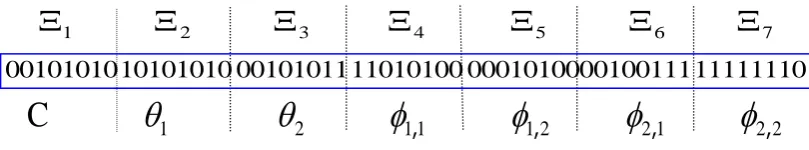
In the GA, each of these variablea is represented by a splice of 8 bits – each bit taken from the

binary set: {0, 1}. For example, considering a network with just two signalised junctions, each

having two stages, the number of splices () is 7. These splices will be combined to form a

chromosome representing a vector of feasible signal setting parameters for the network. For

the example mentioned above, the corresponding chromosome, splices, and represented

variables are given in FIGURE 3. The general form of such a chromosome is shown in

FIGURE 4 for a network with N signalised junctions.

[INSERT FIGURE 3 HERE]

[INSERT FIGURE 4 HERE]

3.2 Chromosome encoding and constraint representation

This section describes how the chromosome decoding is carried out, and how the constraints

given by (3) to (6) are handled in GA-FITSUM. The decoding scheme is based on Ceylan and

Bell (2004).

a. Cycle time: is the proportion of the difference C_max C_min as defined by the first splice

on the chromosome, plus C_min.

 

) (

1

28 max min

min C C

C

C m 

  

where: ( m) = base 10 equivalent of splice m (m) ‡

Cmax = 120 seconds and

Cmin is calculated using (8)

b. Offset: for a stage at a junction h, it is the proportion of the cycle time as defined by

splice m on the chromosome.

 

C

m h

1 28 





 m 2,3,,N1 (13)

where: hm1;

c. Green times: are defined as the sum of the minimum stage length and the proportion of

the remaining green time h r, ,max  h r, ,minas follows:

 

 



 ; m N2,N3,..., (14)

where:



     1 1 1 h y y S N

x is constant at junction h

x m

r   , is a stage at junction h

N

h1,2,...,

3.3 Initialization

The initial set of chromosomes (size of P ) is randomly generated after network specific

information such as the numbers of signalised junctions (N) and stages at each junction (Sh)

have been extracted to determine  (see (11)).

‡ _{For a base 2 number, B, of 8 digits}





8 7 6..._{1 2}

b b b b where b_k 

 

8

1

1

( k* 2k )

k

B b 



 



3.4 Evaluation/fitness

Each chromosome is decoded and sent to the assignment model to obtain corresponding UE

link flows and the associated total travel time, TT. GA-FITSUM then uses TT as the fitness

function for the selection process.

3.5 Selection

In the Selection stage, GA-FITSUM uses the linear ranking approach proposed by Whitley

(1989) for sampling the intermediate population which will then be modified by GA operators

(Sections 3.6 and 3.7). The chromosomes are firstly ranked in an ascending TT order and a

“stochastic sampling with replacement” (Goldberg, 1989) is then carried out using a roulette

wheel that uses probabilities, pk, based on the rank, k, of each chromosome in a generation –

see (15). That is to say,

              ) 1 ( * ) 2 2 ( 2 1 P k P c c P

p_{k w w} (15)

where cw  [1,2] is the “selection bias”– higher values favour the better fit chromosomes

during sampling.

As part of the selection procedure, elitism is applied which ensures the best performing

chromosomes from the preceding generation are always included in the next generation

without any alteration. The parameter Elite controls the number of such chromosomes which

are passed to the next generation.

3.6 Crossover

During crossover, the elite chromosomes are made present in the breeding pool to share their

good performing genes. Each chromosome in the intermediate population is assigned a

probability of Pc to exchange its genetic materials. Those selected are randomly paired for

which GA-FITSUM uses uniform crossover (Syswerda, 1989). Accordingly a mask

mask chromosome determines which parent chromosome supplies the bit for a certain

position in the chromosomes of their two offspring. The unselected chromosomes will be

passed directly to the mutation process.

3.7 Mutation

The probability of mutation, Pm, determines the likelihood of mutation occurring on a certain

chromosome. For those selected, the mutation is implemented by selecting a random point

(bit) on the offspring’s chromosome length and then changing the value of the that bit to 0 if it

was 1, or vice versa.

4 Case Study Application

GA-FITSUM’s performance is considered here, both in terms of the GA search process and in

terms of the optimality of the solution obtained in comparison with a traffic signal

optimisation process that does not anticipate re-routing. The evidence for this study arises

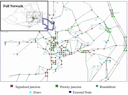
from applications to the road network for the city of Chester in the UK, as illustrated in

FIGURE 5. This network has 75 signalised junctions, 18 roundabouts, and 86 priority

junctions, forming parts of the routes of the various trips in the network. It caters for a total

demand of 22060 pcu/hour, generated from 132 zones.

[INSERT FIGURE 5 HERE]

4.1 GA Parameters and Performance

According to Whitley (1989), population diversity and selective bias are the two important

issues influencing genetic search. As selective bias is increased – which could be

process – the search focuses on the top individuals to exploit their best performing genes and

leads to a fast convergence. A very high selective bias may result in a premature convergence.

Low selective pressure, on the other hand, focuses on diversity and explorative search

behaviour. In GA-FITSUM such an effect could be implemented by higher values of P , Pm,

and Pc. A higher G would increase the number of chances GA gets to improve on the

solution. Several researchers in the field of evolutionary optimisation have tried to investigate

the effect of the GA parameters so as to define these parameters optimally (see for example

Goldberg, 2002). Unfortunately, the most advanced result on optimal adjustment of GA

parameters has been limited to very simple problems.

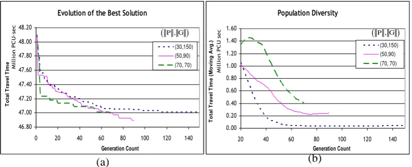
In this paper the performance of GA is presented using the so called “Evolution of Best

Solution” (e.g. FIGURE 6a) and “Population Diversity” (e.g. FIGURE 6b) charts. The former

shows the total travel time resulting from the best solution, in the vertical axis, against the

generation that solution comes from on the horizontal axis. It indicates the speed of solution

convergence. As the Elitism parameter is applied, the solution is observed to improve in

successive generations. Charts of the latter kind show plots of the variance of the total travel

time due to each solution in a generation, smoothed by averaging over a large number of (in

this case 20) generations. It is chosen to indicate the possibility the search has to improve its

solution by incorporating different genes.

[INSERT FIGURE 6 HERE]

FIGURE 6 presents the comparison of different values of the population and generation

number on the search process. The total number of chromosomes (solutions) evaluated has

been constrained to about 4500 so as to see whether it is better to have a larger population size

and thus compromising the generation size, or vice versa. The other parameters were fixed as

with lower values of P in Figure 6b. The relationship between diversity and improvement in

the best solution is clearly evident from the figure. For example, for ( P =30) lower genetic

diversity has limited the search process to fewer improvements after the 60th generation,

whereas a high improvement rate is observed for P =70 in the first few generations. High

and sustained speed of convergence and a better solution are obtained with ( P , G ) equal to

(50, 90).

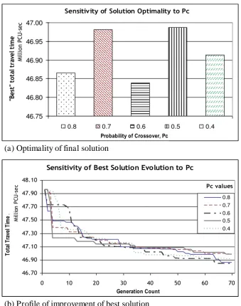
The next parameter tested is the crossover parameter; see FIGURE 7. The values tested are:

0.8, 0.7, 0.6, 0.5, and 0.4. The values of P , G and Pm are fixed at 70, 70 and 0.15,

respectively. The test with Pc=0.6 is shown to provide a better solution than the others.

Similar patterns between solution improvement and diversity are also observed. The high

population diversity up to the 30th generation is associated with faster best-solution

improvement for Pc=0.5. As shown in (c), the diversity decreases with GA evolution except

for Pc=0.4 for which diversity remains about constant after 40 generations.

[INSERT FIGURE 7 HERE]

[INSERT FIGURE 8 HERE]

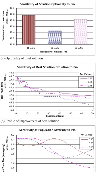
Similarly, the effect of the Pm parameter is presented in FIGURE 8(a-c); values of P , G and

Pc are fixed at 70, 70 and 0.6 respectively. The best solution is found for Pm =0.25. For the

case of Pm,; the effect of different Pm on the diversity of the solutions and the optimal solution

found is, however, rather complex.

4.2 Local Delay Minimising Signal Timings

For comparison, a SATURN based signal optimisation procedure, which will be referred to as

delay is minimized at each intersection using the SATURN simulation model. The method

neither optimises cycle time, nor considers the rerouting effect. After optimum SATOPT

signal times are obtained, traffic is reassigned to take account of drivers’ response to the new

timings. The resulting total travel time is compared with that resulting from GA-FITSUM

timings. In addition, to account for SATOPT not optimising cycle times, and to check how

stage timings and offset optimisations of GA-FITSUM compare with SATOPT, the best

performing common cycle times from GA-FITSUM are also input and compared.

4.3 Results

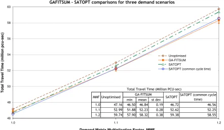
The results from using GA-FITSUM for 3 demand scenarios are presented in Figure 9. The

scenarios are defined by the matrix multiplication factors, MMF, applied on the current year

OD matrix. To account for the effect of different initial random number generating seeds,

GA-FITSUM was run 10 times for each scenario. The mean TT and error bars representing

one standard deviation above and below the mean are plotted in Figure 9. The inset table also

shows the minimum TT obtained from GA-FITSUM. The TT from SATOPT optimised signal

timings with and without the common cycle times are also presented. For benchmarking

purposes, the TT from the un-optimised signal timings are also presented in Figure 9.

As shown in the figure, there does not seem to be much difference between GA-FITSUM and

SATOPT for the first demand scenario. In fact, although the best solution from the 10 runs of

the former gave the smallest TT of 46.5 million pcu-sec, the mean TT from GA-FITSUM

timings is bigger than that resulting from SATOPT timings. For higher levels of demand,

however, it can be seen that GA-FITSUM gives better results than SATOPT does.

SATOPT performs better when the common cycle time from the best performing

GA-FITSUM timings are used, than when the initial node-specific signal timings are in operation.

When compared with GA-FITSUM’s best performing timings, SATOPT results in marginal

increases in TT which get bigger for higher levels of network congestion. This is because it

does not consider the response of the traffic to the changed times.

To see the effect of not anticipating rerouting when optimising signal times, the best

performing signal times and, implicitly, link flows for the first demand scenario is given as

input. For the optimum cycle time determined by GA-FITSUM, SATOPT calculated

optimum stage lengths and offsets after which the traffic was reassigned. FIGURE 10 shows

the difference in link flows as a result of the (new) SATOPT timings, which is unaccounted

for in the conventional optimisation calculations which do not anticipate rerouting. For the

case tested, the associated increase in TT is 0.5 million pcu-sec per hour (which is around

25,000 pcu-hr of delay annually).

5 Conclusions

In this paper, a GA based method was presented for optimising traffic signals in a way that

anticipates re-rerouting of traffic, and its application on the city of Chester was presented. The

GA based method has given promising results in finding optimum signal timings with stable

flows.

When compared to a local delay minimizing timings, the process by which routing is

anticipated has given better results for the network considered in this paper. The

improvements after considering rerouting are relatively bigger when there is a higher level of

varying levels of congestion, to explore the improvements associated with considering routing

in optimising signal timings.

A GA based method should be run several times using different initial random seeds to better

handle solution convergence issues. This will significantly increase the relatively long

computing time associated with the use of GA. The combination of population size,

probabilities of crossover and mutation as well as the chromosome design contributes to how

GA performs. The question of how to find optimum values of the GA parameters is still a

difficult issue and requires further research.

ACKNOWLEDGMENTS

This study was sponsored by the Norwegian Council of Universities' Committee for

Development Research and Education, NUFU. We would like to acknowledge the detailed

comments of all six anonymous referees, which helped us in improving an earlier version of

REFERENCES

Abdulaal, M., & LeBlanc, L. J. (1979), Continuous equilibrium network design models,

Transportation Research Part B, 13(1), 19-32.

Abu-Lebdeh, G. & Benekohal, R.F. (2003), Design and evaluation of dynamic traffic

management strategies for congested conditions, Transportation Research Part A, 37(2),

109-127.

Almond, J. & Lott R. S. (1968), The Glasgow Experiment: implementation and assessment.

Road Research Laboratory Report 142, Road Research Laboratory, Crowthorne.

Allsop, R.E. (1974), Some possibilities for using traffic control to influence trip distribution

and route choice, in Buckley D. J., Ed., Proc. 6th Int. Symp. on Transport and Traffic

Theory, Elsevier, New York, 345-373.

Balling, R., Powell, B., and Saito, M. (2004) Generating future land-use and transportation

plans for high-growth cities using a genetic algorithm, Computer-Aided Civil and

Infrastructure Engineering, 19 (3), 213-222.

Ben Ayed, O., Boyce, D. E. & Blair III, C.E. (1988), A general bi-level linear programming

formulation of the network design problem, Transportation Research Part B, 22(4),

311-318.

Bergendorff, P., Hearn, D. W., & Ramana, M. V. (1997), Congestion toll pricing of traffic

networks, in Pardalos P. M., Hearn D. W., and Hager W. W., Eds., Lecture Notes in

Economics and Mathematical Systems,.450: Network Optimization, Springer, Berlin, 51-71.

Bielli M., Caramia M., & Carotenuto P. (2002), Genetic algorithms in bus network

optimization, Transportation Research Part C, 10(1), 19-34.

Ceylan H. & Bell M. G. H. (2004), Traffic signal timing optimisation based on genetic

algorithm approach, including drivers’ routing, Transportation Research Part B, 38(4),

Chakroborty, P. (2003), Genetic algorithms for optimal urban transit network design,

Computer-Aided Civil and Infrastructure Engineering, 18(3), 184-200.

Chakroborty, P., Deb, K. & Srinivas, B. (1998), Network-wide optimal scheduling of transit

systems using genetic algorithms, Computer-Aided Civil and Infrastructure Engineering

13(5), 363-376.

Charypar, D. & Nagel, K. (2005), Generating complete all-day activity plans with genetic

algorithms, Transportation, 32(4), 369-397.

Chiou, S-W. (1999), Optimization of Area Traffic Control for Equilibrium Network Flows.

Transportation Science 33(3), 279-289.

Cree N.D., Maher M.J. & Paechter B. (1998), The continuous equilibrium optimal network

design problem: a genetic approach, in M.G.H. Bell, Ed., Transportation Networks: Recent

Methodological Advances, Pergamon, Oxford, 163-174.

Daganzo, C. F. and Sheffi, Y. (1977) On stochastic models of traffic assignment,

Transportation Science, 11(3), 253-274.

Dantzig, G. B., Harvey, R. P., Landsdown, Z. F., Robinson, D. W. & Maier, S. F. (1979),

Formulating and solving the network design problem by decomposition, Transportation

Research Part B, 13(1), 5-17.

Foy, M., R. F. Benekohal, & D. E. Goldberg (1992), Signal timing determination using

genetic algorithms, Transportation Research Record, 1365, 108-115.

Friesz, T.L., Cho, H.J., Mehta, N.J., Tobin, R. & Anandalingam, G. (1992), A simulated

annealing approach to the network design problem with variational inequality constraints.

Transportation Science, 26, 18-26.

Friesz, T.L. & Harker, P.T. (1985), Properties of the iterative optimisation-equilibrium

Friesz, T.L., Tobin, R.L., Cho, H.J., & Mehta, N.J. (1990), Sensitivity analysis based heuristic

algorithms for mathematical programs with variational inequality constraints, Mathematical

Programming, 48, 265-284.

Goldberg D.E. (1989), Genetic Algorithms in Search, Optimisation, and Machine Learning,

Addison Wesley Longman Inc., Reading, Mass.

Goldberg D.E. (2002), The Design of Innovation: Lesson from and for competent genetic

algorithms, Kluwer Academic Publishers, Boston.

Girianna, M. & Benekohal, R. (2004), Using genetic algorithms to design signal coordination

for oversaturated networks, Intelligent Transport Systems Journal, 8(2), 117-129.

Hearn, D. W., & Ramana, M. V. (1998), Solving congestion toll pricing models, in Nguyen S.

and Marcotte P., Eds., Equilibrium and Advanced Transportation Modeling, Kluwer

Academic Publishers, Boston, 109-124.

Hunt, P.B., Robertson, D.I., Bretherton, R. D., & Winton, R. I. (1981), SCOOT - A traffic

responsive method of coordinating signals, TRRL Laboratory Report 1014, TRRL,

Berkshire, England.

(IHT) Institution of Highways & Transportation (1997), Transport in the Urban Environment.

Institution of Highways & Transportation, London.

Kim H., Baek S. & Lim Y. (2001), Origin-destination matrices estimated with a genetic

algorithm from link traffic counts, Transportation Research Record, 1771, 156-163.

Lawphongpanich, S. & Hearn, D. W. (2004), An MPEC approach to second-best toll pricing,

Mathematical Programming B, 101(1), 33-55.

LeBlanc, L. & Boyce, D. (1986), A bi-level programming for exact solution of the network

design problem with user-optimal flows, Transportation Research Part B, 20(3), 259-265.

Lee, C. (1998) Combined Traffic Signal Control and Traffic Assignment: Algorithms,

Implementation and Numerical Results, Ph.D. Dissertation, the University of Texas at

Lo, H.K., Chang, E & Chan, Y.C. (2001), Dynamic network traffic control, Transportation

Research Part A, 35(8), 721-744.

Luo, Z., Pang, J.S., & Ralph, D. (1996), Mathematical Programs with Equilibrium

Constraints, Cambridge University Press, New York.

Marcotte, P. (1981), An analysis of heuristics for the continuous network design problem, in

Hurdle, V. F. et al., Eds., Proceedings of the 8th International Symposium on Transportation

and Traffic Theory, University of Toronto Press, Toronto, 27-34.

Marcotte, P. (1986), Network design problem with congestion effects: a case of bi-level

programming, Mathematical Programming, 34, 142 – 162.

Meng, Q., Yang, H., & Bell, M.G.H. (2001), An equivalent continuously differentiable model

and a locally convergent algorithm for the continuous network design problem,

Transportation Research Part B, 35(1), 83-105.

Park, B., Messer C.J., & Urbanik T. (2000), Enhanced genetic algorithm for signal timing

optimization of oversaturated intersections, Transportation Research Record, 1727, 32-41.

Park, B. and Yun, I. (2005). Stochastic Optimization Method for Coordinated Actuated Signal

Systems. Final Report of ITS Center Project: Evaluation of advanced traffic signal

controllers. Center for Transportation Studies, University of Virginia, USA.

Robertson, D. I. (1969), ‘TRANSYT’ method for area traffic control, Traffic Engineering and

Control, 10, 276 – 281.

Sharma, S., Lingras, P. & Zhong, M. (2004), Effect of missing values estimations on traffic

parameters, Transportation Planning and Technology, 27(2), 119-144.

Shepherd, S.P. & Sumalee A. (2004), A genetic algorithms based approach to optimal toll

level and location problems, Networks and Spatial Economics, 4, 161-179.

Smith, M.J. (1979), The existence, uniqueness and stability of traffic

Stathopoulos, A. & Tsekeris, T. (2004), Hybrid meta-heuristic algorithm for the simultaneous

optimization of the O-D trip matrix estimation, Computer-Aided Civil and Infrastructure

Engineering, 9(6), 421-435.

Steenbrink, P. A. (1974), Optimization of Transport Networks, John Wiley & Sons, London.

Srinivasan, D., Cheu, R.L., Poh, Y.P. & Ng, A.K.C. (2000), Development of an intelligent

technique for traffic network incident detection, Engineering Applications of Artificial

Intelligence, 13(3), 311-322.

Sumalee, A. (2004), Optimal road user charging cordon design: a heuristic optimisation

approach, Computer-Aided Civil and Infrastructure Engineering, 19(5), 377-392.

Suwansirikul, C., Friesz, T. L., & Tobin R. L. (1987), Equilibrium decomposed optimization:

a heuristic for the continuous equilibrium network design problem, Transportation Science,

21(4), 254-263.

Syswerda, G. (1989), Uniform crossover in genetic algorithms, Proc. 3rd Intl. Conf. Genetic

Algorithms, Morgan Kaufmann, 2-9.

Taale, H. and Van Zuylen, H.J. (2003). The Effects of Anticipatory Traffic Control for

Several Small Networks. Paper presented at 82nd Transportation Research Board Annual

Meeting, Washington DC, January 12th–16th 2003.

Van Vliet, D. (1982), SATURN - A modern assignment model, Traffic Engineering and

Control, 23, 578-581.

Varia, H.R. and Dhingra S.L. (2004). Dynamic Optimal Traffic Assignment and Signal Time

Optimization Using Genetic Algorithms. Computer-Aided Civil and Infrastructure

Engineering 19, 260-273.

Verhoef, E. T. (2002), Second-best congestion pricing in general networks: heuristic

algorithms for finding second-best optimal toll levels and toll points, Transportation

Wardrop J. G. (1952), Some theoretical aspects of road traffic research, Proc. Institution of

Civil Engineers, 1(2), 325-378.

Whitley, D. (1989), The GENITOR algorithm and selection pressure: Why rank based

allocation of reproductive trial is best, in Schaffer, J., Eds., Proc. of the 3rd Intl. Conf. on

Genetic Algorithms, Morgan Kaufmann, 116-121.

Webster F.V. (1958), Traffic Signal Settings, Road Research Technical Paper No. 39, HMSO,

London.

Yang, H. (1997), Sensitivity analysis for the elastic-demand network equilibrium problem

with applications, Transportation Research Part B, 31(1), 55-70.

Yin Y. (2000), Genetic algorithms-based approach for bi-level programming models, ASCE

FIGURE 1 Signal design variables for junction h

GREEN

AMBER

RED

Cycle Time (C)

KEY

Offset (h)

Green time 1 (h,1)

phase 1

phase 2

Inter-green 1 (Ih,1)

Green time 2 (h, 2)

phase Sh

Green time Sh

h

s h,



FIGURE 2 GA-FITSUM Flow Chart

Is i < P ?

No No

INITIALIZATION

(i. e. generate P feasible solutions randomly)

EVALUATION

CALCULATE TOTAL TRAVEL TIME

PICK THE OPTIMUM SOLUTION

Yes

Yes

FIND THE EQUILIBRIUM FLOW PATTERN

(i. e. run SATURN)

Next so

lu

tio

n,

i =

i+

1

SELECTION

Linear Ranking & Elitism

CROSSOVER AND MUTATION

Is g < G ?

Next g

enerati

on

o

f so

lut

ion

s,

g

=

g +

FIGURE 3: Splices, Chromosome, and represented variables – an illustrative example

2 2 1

2 2

1 1

1 2

1













C

7 6

5 4

3 2

1















11111110 0100111

0 00010100 11010100

00101011 10101010

FIGURE 4: Chromosome Structure

|

...,

,

|

...

|

,...,

,

|

...,

,

,

|

|

1 N N Sn

S N

FIGURE 5: Layout of the Chester network

Signalised junction Priority junction Roundabout

Zones External Node

FIGURE 6: Comparison of different ( P , G ) values

(a) profile of improvement of best solution (b) moving average (per 20 generations) of the variance in the total travel times of solutions in each generation

(a) (b)

Evolution of the Best Solution

46.80 47.00 47.20 47.40 47.60 47.80 48.00 48.20

0 20 40 60 80 100 120 140

M il li o n P C U -s e c Generation Count T o ta l T ra v e l T im e a (30,150) (50,90) (70, 70)

P ,G

Population Diversity 0.00 0.20 0.40 0.60 0.80 1.00 1.20 1.40 1.60

20 40 60 80 100 120 140

M il li o n P C U s e c Generation Count T o ta l T ra v e l T im e ( M o v in g A v g .) a (30,150) (50,90) (70, 70)

Sensitivity of Solution Optimality to Pc 46.75 46.80 46.85 46.90 46.95 47.00 (30 M il li o n P C U -s e c

Probability of Crossover, Pc

"B e st " to ta l tr av e l ti m e

0.8 0.7 0.6 0.5 0.4

(a) Optimality of final solution

Sensitivity of Best Solution Evolution to Pc

46.70 46.90 47.10 47.30 47.50 47.70 47.90 48.10

0 10 20 30 40 50 60 70

M il li o n P C U -s e c Generation Count T o ta l T ra ve l T im e . 0.8 0.7 0.6 0.5 0.4 Pc values

(b) Profile of improvement of best solution

Sensitivity of Population Diversity to Pc

0.40 0.60 0.80 1.00 1.20 1.40 1.60

20 30 40 50 60 70

M il li o n s P C U s e c Generation Count T o ta l T ra ve l T im e ( M o vin g A vg .) . 0.8 0.7 0.6 0.5 0.4 Pc values

(c) Moving average (per 20 generations) of the variance in the fitness values of solutions in each generation

Sensitivity of Solution Optimality to Pm 46.0 46.2 46.4 46.6 46.8 47.0 47.2 1 M il li o n P C U -s e c

Probability of Mutation, Pm

"O p ti m u m " to ta l tr a v e l ti m e

0.35 0.25 0.15

(a) Optimality of final solution

Sensitivity of Best Solution Evolution to Pm

46.2 46.4 46.6 46.8 47.0 47.2 47.4 47.6 47.8 48.0 48.2

0 10 20 30 40 50 60 70

M il li o n P C U -s e c Generation Count To ta l Tra v e l Ti m e 0.35 0.25 0.15 Pm Values

(b) Profile of improvement of best solution

Sensitivity of Population Diversity to Pm

0.4 0.5 0.6 0.7 0.8 0.9 1.0 1.1 1.2

20 30 40 50 60 70

M il li o n P C U s e c Generation Count To ta l Tr av el Ti m e (M ov ing A vg. ) 0.35 0.25 0.15 Pm values

(c) Moving average (per 20 generations) of the variance in the fitness values of solutions in each generation

GAFITSUM - SATOPT comparisons for three demand scenarios

46 48 50 52 54 56 58 60

1.0 1.1 1.2

Demand Matrix Multiplication Factor, MMF

Total

Travel

Time

(mi

ll

ion pcu-sec)

Unoptimised GA-FITSUM SATOPT

SATOPT (common cycle time)

min mean st dev

1.0 47.16 46.50 46.84 0.19 46.72 46.56

1.1 52.99 51.88 52.23 0.28 52.62 52.25

1.2 59.74 57.90 58.32 0.38 59.38 58.55

SATOPT (common cycle time) GA-FITSUM

Total Travel Time (Million PCU-sec)

MMF Unoptimised SATOPT

Figure 9 Total travel time comparison of SATOPT and GA-FITSUM

FIGURE 10: Difference in link flows as a result of SATOPT timings (pcu/hour)

TABLE 1 Notation

L Number of links

qa flow on link a (a = 1,2,…,L)

Tij total demand for travel between origin i and destination j

C common cycle time

h offset at junction h, element of the vector of offsets 

hr duration of the green time for stage r at junction h, element of green time vector



 (C, , ) a vector of signal setting parameters (i.e. cycle time, offsets, and stage lengths)

q*() the vector of user equilibrium link flows gjven signal setting parameters  fijp flow between origin i and destination j on route p

ta (, q*() ) travel time on link a

tijp total travel time on route p from origin i to destination j

TT total network travel time

Sh total number of stages at junction h

Ih,r for junction h, the intergreen between the end of the green time for stage r and

the start of the next green

G generation counter

 base 2 to base 10 converting function

 total number of signal setting variables in a network.

m the mth splice in a chromosome (e.g. 1 = the first 8 bits); see Section 3.1.

P population size G generation number cw selection bias