This is a repository copy of
Efficient simulations for automotive design
.
White Rose Research Online URL for this paper:
http://eprints.whiterose.ac.uk/133872/
Version: Accepted Version
Proceedings Paper:
Konefal, T, Marvin, A C orcid.org/0000-0003-2590-5335, Dawson, J F
orcid.org/0000-0003-4537-9977 et al. (1 more author) (2005) Efficient simulations for
automotive design. In: Workshop on "SAFETEL – Safe Electromagnetic
Telecommunications on Vehicles". EMC Europe Workshop 2005. EMC Europe Workshop
2005, 19-21 Sep 2005 , ITA , pp. 19-21.
[email protected] https://eprints.whiterose.ac.uk/
Reuse
["licenses_typename_other" not defined]
Takedown
If you consider content in White Rose Research Online to be in breach of UK law, please notify us by
Abstract—Some preliminary results are presented for the
statistical coupling of EM radiation to a transmission line inside a lossy chamber with an aperture. The rapid Intermediate Level Circuit Modelling (ILCM) technique has been used to obtain the results, which have relevance to the calculation of the probability of failure of a vehicle subsystem
in situ.
Index Terms—Circuit Modelling, Statistical Coupling,
Transmission Lines.
I. INTRODUCTION
OR a typical subsystem fitted inside a vehicle, the most significant threat to its operational integrity arises as a result of intentional transmitters such as mobile phones or other vehicle radio communications equipment, in close proximity to the subsystem. For example, a mobile phone operating at 2W radiated power inside the vehicle will induce higher currents in vehicle internal wire looms and circuitry than an external plane wave threat field of amplitude 100Vm-1 [1]. Many sensitive vehicular subsystems will have been designed with some degree of EMC in mind, and it is unlikely that radiation on to the equipment per se will be the major source of interference to system operation. Instead, the major route by which electromagnetic interference (EMI) will enter a subsystem is likely to be via cabling that enters and exits the subsystem. Such cabling will generally be either of a communications/control nature or supply power to the subsystem. In both cases the cables may act as efficient antennas, particularly at frequencies where the free space wavelength is comparable to or shorter than the cable length. The energy picked up by such cables will in most cases be the major source of EMI for subsystems attached to the cables, as the energy is directed into the subsystems by a transmission line effect. Screening of cables can help enormously, but cannot detract from the physical reality that a cable resembles a receiving antenna.
In this paper we present some preliminary results of a rapid Intermediate Level Circuit Modelling (ILCM) tool that can be used to predict the EM signals picked up by a transmission line in close proximity to the wall of a
T. Konefal is with the Electronics Department of the University of York, Heslington, York, UK (phone: +44 1904 432406; fax: +44 1904 433224; e-mail: [email protected]).
A.C. Marvin, J.F. Dawson and M.P. Robinson are also with the Electronics Department of the University of York, Heslington, York, UK (e-mail: [email protected] , [email protected] and [email protected] respectively).
The ILCM tool described here was developed with financial support from BAE Systems. Many thanks to Ian MacDiarmid.
rectangular metal chamber. The metal chamber contains a rectangular aperture, and is irradiated externally by a plane wave. In the context of vehicle EMC, the rectangular chamber and aperture are analogous to the metallic car body with windows, while the transmission line pressed up against the chamber wall is analogous to a wire loom pressed up against the metallic vehicle body, carrying signals or power between vehicle subsystems.
The statistical nature of the signal picked up by a transmission line inside a lossy chamber is investigated using the ILCM technique, both as a function of varying frequency and position. In the latter case, a statistical analysis is impractical using traditional numerical methods such as Method of Moments (MoM), Finite Difference Time Domain (FDTD) or Transmission Line Matrix (TLM), due to the prohibitive time scales involved. For example, using TLM for just one deterministic transmission line position typically takes 3-4 hours to reach a solution for a few hundred frequency points. In contrast, the ILCM technique takes a few milliseconds per arbitrary frequency point and deterministic transmission line position. This makes a statistical analysis involving a few thousand sample positions feasible within a timescale of a few tens of seconds.
A general framework is outlined whereby the results of the ILCM statistical analysis can be used to determine the probability of failure or upset of a vehicular subsystem, with the subsystem fitted inside the vehicle and the vehicle irradiated by a known field strength. In order to calculate this probability, it is first necessary to establish an immunity profile for the vehicle subsystem. This process is described in Section II. Section III describes the statistical results of the ILCM method, with some general recommendations on their use being made in Sections IV and V.
II. IMMUNITY PROFILE MEASUREMENT
In view of the fact that the dominant mechanism for EMI ingress into a vehicle subsystem is likely to be via the cabling, it is proposed that the bulk current injection (BCI) technique be used to inject an interference signal on to a cable leading to an equipment under test (EUT), as in Fig. 1. For a digital equipment, the onset of an immunity problem can be anticipated by monitoring the rate of intermodulation product (IP) increase with increasing BCI signal. At a signal level approximately 5dB below a failure mode the IP/BCI signal relationship begins to deviate from the nominal linear, quadratic, cubic etc. dependence
Efficient Simulations for Automotive Design
T. Konefal, A.C. Marvin, J.F. Dawson and M.P. Robinson
F
2
(depending on the particular harmonic of the BCI signal involved), and indicates that the EUT is being stressed into a highly non-linear regime [2]. Such IPs can be monitored either by a small sensing monopole inside the EUT or by a spectrum analyser at the other end of the cable, as in Fig. 1. An oscilloscope can also be used to monitor the presence of jitter in the digital output signal; such jitter increases with increasing BCI signal and can be used as a second identifier of interference [3]. More generally, for both digital and analogue equipment, the EUT can be monitored for anomalous behaviour as the BCI threat signal is increased. In this way, a voltage immunity profile Vimm(ω)can be built up for the EUT as a function of frequency: if the signal level Vimm(ω) is exceeded the EUT is deemed to malfunction.
Spectrum Analyser
Digital EUT
IP monitoring
monopole
Vehicle chassis
Termination Spectrum Analyser or Oscilloscope
[image:3.595.48.290.77.340.2]BCI device
Figure 1. Proposed experimental set up to measure immunity profile.
III. STATISTICAL TREATMENT OF FIELD INGRESS INTO VEHICLES
The actual threat signal induced on a wire loom inside a vehicle due to an EM emission, either from within the vehicle or from the vehicle exterior, is a poorly posed deterministic problem. It is well known [4] that even very small changes in the position of the transmitter or receiving wire loom (and indeed any other sizeable metallic objects within the vehicle) can alter the signal picked up by the wire loom significantly. Instead, the signal picked up by the wire loom (regarded as a transmission line) can be treated in a statistical manner above a frequency corresponding to the 60th consecutive (in frequency) resonant cavity mode of the vehicle/chamber [5].
The University of York has recently developed a very rapid Intermediate Level Circuit Modelling (ILCM) tool, which can predict the level of interference induced on arbitrary terminations of a transmission line inside a rectangular box with an aperture, irradiated externally by a plane wave. Losses in the box can be controlled by assigning an arbitrary electric field reflection coefficient to one of the box walls. Typical results for the coupling to a 65cm long transmission line inside a box of size 60
×
30×
90cm3 containing an aperture of size 30×
3cm2 and a back wall with electric field reflection coefficient ρ=−0.5 are shown in Fig. 2. The internal transmission line has characteristic impedance 126.6Ω and is terminated at each end in aΩ
50 load, while the box is irradiated externally by a 1Vm -1
peak field. The results of TLM simulation are given in Fig. 2 for comparison. The tremendous advantage of the ILCM technique is that it is 3-4 orders of magnitude faster than TLM in obtaining a result. For example, TLM will typically take several hours to produce a result as in Fig. 2,
whereas the ILCM model will take only a few seconds. We note that the TLM results below about 250MHz are likely to be inaccurate, due to the necessary finite and premature curtailment of the time domain response to the TLM Gaussian pulse excitation. The effect of this is to overestimate the low frequency Fourier transformed response. Also, we have deliberately chosen a small model since TLM simulation up to 3GHz of a full size vehicle would be impractical within a sensible time scale. A full size model using the ILCM technique however is entirely feasible.
-160 -140 -120 -100 -80 -60 -40 -20
0 500 1000 1500 2000 2500 3000
Received Power (dBm)
Frequency (MHz)
[image:3.595.314.545.186.338.2]Circuit Model TLM
Figure 2. Coupling to transmission line termination in large lossy box.
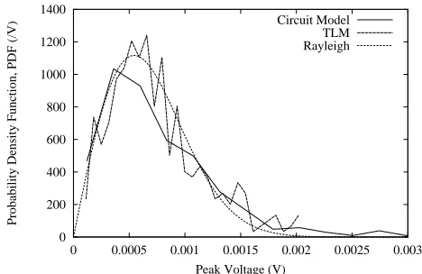
0 200 400 600 800 1000 1200 1400
0 0.0005 0.001 0.0015 0.002 0.0025 0.003
Probability Density Function, PDF (/V)
Peak Voltage (V)
[image:3.595.55.287.244.346.2]Circuit Model TLM Rayleigh
Figure 3. Statistics of voltage induced across load at end of transmission line inside large lossy box with aperture (see Figure 2). Frequency range
considered is 1.25GHz to 3GHz.
The statistical nature of the power received by the transmission line is evident from the rapid fluctuations in power in Fig. 2 above a frequency of about 1.25GHz. The resonant frequency of the 60th consecutive cavity mode lies just below 1.25GHz, so that above this frequency a statistical treatment is appropriate [5]. The Probability Density Function (PDF) of the voltage induced at the termination of the line in Fig. 2 in the frequency range 1.25GHz-3GHz is replotted in Fig. 3, where it can be seen that agreement with TLM is generally very good, despite the relatively low number (438) of data points involved. Superficially, the distribution resembles the Rayleigh distribution,
−
= 2 22
2 exp )
(
σ σ
x x
x
[image:3.595.312.546.367.519.2]which is plotted in Fig. 3 for comparison. A least mean square error (LMSE) fitted value of
σ
=0.543mV is obtained with the circuit model, with a value of555 . 0 =
σ
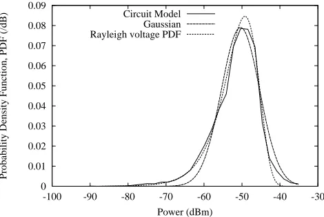
mV being obtained for the TLM simulation. On a logarithmic scale, the power in dBm appears to follow a normal distribution,− − = 2 2 2 ) ( exp 2 1 ) ( g g g x x f σ µ π
σ (2)
as in Fig. 4. LMSE fitted values of
σ
g =6.08dB and9 . 53
− =
µ dBm are obtained for the normal distribution fit to the ILCM data in Fig. 4. This result is in general agreement with the observation made in [6] that the PDF of the power induced in representative vehicular cables follows an approximate log-normal distribution (at least as a function of position), with a typical standard deviation in the range 3-6dB. Note however that it is not entirely consistent with the (possibly over simplistic) assumption of Rayleigh statistics in the transmission line terminal voltage in Fig. 3. The latter assumption results in a logarithmic power distribution with a mode that is slightly skewed to the right, also indicated in Fig. 4 (the ILCM LMSE value
543 . 0 =
σ
mV is assumed).0 0.01 0.02 0.03 0.04 0.05 0.06 0.07 0.08 0.09
-100 -90 -80 -70 -60 -50 -40 -30
Probability density function, PDF (/dB)
Power (dBm) Circuit model
[image:4.595.310.547.304.461.2]Gaussian Rayleigh voltage PDF
Figure 4. Comparison of ILCM data of Fig. 2 above 1.25GHz with a normal (Gaussian) distribution and the power distribution resulting from a Rayleigh
voltage distribution. 0 0.01 0.02 0.03 0.04 0.05 0.06 0.07 0.08 0.09
-100 -90 -80 -70 -60 -50 -40 -30
Probability Density Function, PDF (/dB)
Power (dBm) Circuit Model
Gaussian Rayleigh voltage PDF
Figure 5. ILCM simulation of PDF of coupling to transmission line for random variations in position.
Similar results are obtained with regard to random variations in the position of the internal transmission line.
For example, Fig. 5 shows the PDF of the power (in dBm) developed in the 65cm long transmission line at 2.5GHz, for 10,000 random positions of the transmission line inside the box. In this case the transmission line is terminated at each end in its characteristic impedance of 126.6Ω. The LMSE best fit parameters are σg =5.04dB,
4 . 50 − =
µ
dBm for the normal distribution and23 . 1
=
σ mV for the Rayleigh voltage PDF. Once again, we note a skew to the right in the mode of the Rayleigh voltage PDF, and this is in fact also present in the ILCM results. Note however that when plotted on a logarithmic ordinate scale (Fig. 6), it is the Gaussian (normal) distribution which better replicates the upper tail end of the ILCM distribution. This is significant when it comes to predicting the probability of failure of a vehicular subsystem attached to the cable, since it is the upper tail of the distribution which determines the probability of failure when the latter is relatively low (say less than 10%). The use of such a PDF in predicting the failure probability is outlined in the following section. 1e-016 1e-014 1e-012 1e-010 1e-008 1e-006 0.0001 0.01 1
-100 -90 -80 -70 -60 -50 -40 -30
Probability Density Function, PDF (/dB)
Power (dBm)
[image:4.595.55.287.363.516.2]Circuit Model Gaussian Rayleigh voltage PDF
Figure 6. ILCM simulation of PDF of coupling to transmission line for random variations in position (log plot).
IV. PROBABILISTIC SAFETY MARGIN
The statistical ILCM approach to finding the distribution of voltage presented to a vehicular subsystem attached to a wire loom/transmission line inside a vehicle can be combined with other published literature [4][7][8] to provide us with a probability that the vehicle subsystem will experience an immunity problem in situ. If we regard the vehicle as a metallic box containing electrically large apertures (the windows), the analysis presented in [7] gives the mean shielding effectiveness (SE) of the vehicle as
= Q V tλ σ π 2 log 10
SE(dB) 10 (3)
where V is the volume of the interior of the vehicle, Q is the quality factor of the cavity (a means of calculating Q is presented in [7]), and
λ
is the free space wavelength. For an electrically large window,σ
t takes the formi
t A θ
[image:4.595.54.289.566.723.2]4
where A is the physical aperture (window) area and
θ
i isthe angle of incidence. Several windows require several terms of the form given in (4), all added together. If we regard the vehicle as a lossy reverberation chamber, we can use the results of [4] to relate the mean field in the chamber as calculated by (3) to the most probable field in the chamber (vehicle). Specifically, [4] enables us to relate the latter field to the most probable single component of field (e.g. Ex ), which is found both theoretically and
experimentally to be Rayleigh distributed. The single component of electric field is relevant to the coupling of energy to a wire loom transmission line pressed up against the metal vehicle chassis. Indeed, it is shown in [9] that the single (normal) component of field at the vehicle chassis is actually about twice the value of the single component of field in the general interior of the vehicle. In the ILCM simulations considered here, the distribution of a single component of electric field is also Rayleigh in nature. We can therefore use the results of the ILCM most probable induced voltage/most probable single component of field ratio and multiply this ratio by the most probable single component of field inside the vehicle, as calculated from [4][7]. The result should be the most probable value of induced voltage on the wire loom transmission line when the vehicle subsystem is installed in situ as intended.
Voltage Probability
Density Function
Area under curve is unity
Figure 7. Statistical distribution of voltage entering the EUT in Fig. 1.
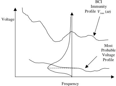
We can combine a knowledge of the most probable transmission line voltage in situ and the detailed PDF of the terminal voltage, with the experimental immunity profile
) (ω imm
V of a vehicular EUT in Section II, in order to predict the probability that the EUT will experience an immunity problem in situ. Figures 7 and 8 illustrate the principles involved, and are based on material presented in [8]. Fig. 7 shows an approximate statistical distribution of voltage at the cable termination (EUT end) in Fig. 1, when the EUT is installed in the vehicle and irradiated by a known field. Fig. 8 illustrates how this profile, and the variation of its most probable value with frequency can be combined with the immunity profile Vimm(ω) of the EUT. It is evident that the probability of malfunction or failure of the EUT is given by the area under the tail of the voltage statistics profile curve at the point where the curve intersects the immunity profile curve as obtained by measurement using the BCI technique. As the threat field increases, the most probable voltage in the statistical voltage profile of Fig. 8 moves proportionally up the ordinate, while the immunity profile remains stationary. The overall result is that a greater area of the tail of the PDF is encapsulated by the point of intersection of the two
curves, indicating that the probability of failure has increased. In this way, the probability of failure of the vehicle subsystem (EUT) may be determined both as a function of frequency and incident threat field level, when the subsystem is installed on the vehicle as intended.
Voltage
Frequency
BCI Immunity Profile Vimm(ω)
Most Probable
[image:5.595.323.525.118.267.2]Voltage Profile
Figure 8. Use of PDF in Fig. 7 together with measured immunity profile of EUT to determine the probability of failure for a given radiated threat level.
V. CONCLUSION
The ILCM technique can be used as a rapid means of obtaining the statistical distribution of voltage or power delivered to a vehicular subsystem attached to internal wire looms, when the vehicle is submitted to external EMI. The significant high power ‘tail end’ of the PDF appears to be log-normally distributed, and can be used to predict the probability of failure of the vehicular subsystem in situ. Such information is directly relevant to the performance of a risk assessment for failure of the vehicular subsystem.
REFERENCES
[1] Deliverable 3.1, SAFETEL project. Available from http://www.safetel-project.com
[2] I.D. Flintoft, A.C. Marvin, M.P. Robinson, K. Fischer and A.J. Rowell, “The re-emission spectrum of digital hardware subjected to EMI,” IEEE
Transactions on Electromagnetic Compatibility, vol. 45, no. 4,
November 2003, pp. 576-585.
[3] M.P. Robinson, K. Fischer, I.D. Flintoft and A.C. Marvin, “A simple model of EMI-induced timing jitter in digital circuits, its statistical distribution and its effect on circuit performance,” IEEE Transactions
on Electromagnetic Compatibility, vol. 45, no. 3, August 2003, pp.
513-519.
[4] D.A. Hill, “Electromagnetic theory of reverberation chambers,” National Institute of Standards and Technology (NIST) Technical Note 1506, Technology Administration, US Department of Commerce, December 1998.
[5] M.L. Crawford and G.H. Koepke, “Design, evaluation and use of a
reverberation chamber for performing electromagnetic
susceptibility/vulnerability measurements,” Technical Report Tech. Note 1092, National Bureau of Standards, 1986.
[6] Deliverable 2.2, SAFETEL project. Available from http://www.safetel-project.com
[7] D.A. Hill et al., “Aperture excitation of electrically large, lossy cavities,” IEEE Transactions on Electromagnetic Compatibility, vol. 36, no. 3, August 1994, pp. 169-177.
[8] P.H. Lever, “Automotive electromagnetic susceptibility testing,” MPhil. Thesis, Department of Engineering, University of Warwick, June 1994.
[9] J.F. Dawson et al., “Field statistics in an enclosure with an aperture: effect of Q-factor and number of modes,” IEEE International