Evaluating water sounds to improve the soundscape of urban areas affected by traffic noise

Evaluating water sounds to improve the soundscape of urban areas

affected by traffic noise

Jin Youa), Pyoung Jik Leeb)and Jin Yong Jeonc)

(Received: 16 January 2010; Revised: 7 July 2010; Accepted: 11 July 2010)

The acoustic characteristics of various kinds of water sounds were investigated to evaluate their suitability for improving the soundscape with road traffic in urban spaces. Audio recordings were made in urban spaces with water features such as fountains, streams, water sculptures, or waterfalls. The temporal and spectral aspects of the sounds were clarified, and subjective evaluations were performed to find the proper level difference between water sounds and road traffic noise for making urban soundscape more subjectively pleasant. The results indicated that the perceptual difference of the water sound level was around 3 dB with noises from road traffic in the background. The water sound, which had 3 dB less sound pressure level, was evaluated as preferable when the levels of road traffic noise were 55 or 75 dBA. It was also found that water sounds with relatively greater energy in low-frequency ranges were effective for masking noise caused by road traffic. The results of the present study will be valuable to urban designers and planners by providing guidelines for improving design solutions for water features in urban soundscape. © 2010 Institute of Noise Control Engineering.

Primary subject classification: 52.3; Secondary subject classification: 38.1

1 INTRODUCTION

Water is used as a primary landscape element in urban spaces because water features are visually and aurally attractive. A previous study1 assessed the responses of users of the First National Bank Plaza in Chicago, USA to the services and design features of the plaza. When asked what they liked best about the plaza, the most common response was ‘entertainment,’ but the second most frequent response was the ‘fountain.’ Another study of eight plazas in Los Angeles and San Francisco2 also reported that ‘water features’ or ‘the fountain’ were viewed as positive design attributes of public spaces. Water and foliage are thought to be primary landscape qualities that have special effects on preferences in the visual aesthetic field3. For this reason, urban landscape design guide-lines recommend the introduction of water features to

increase visual interest4. However, studies of the auditory aspects of water are rather limited.

Recently, the use of water features in urban spaces has been considered in the context of the soundscape. Yang and Kang5conducted a case study in the Peace Garden in Sheffield, UK to investigate general percep-tions of urban soundscapes and sound preferences. They found that the sound of water was a ‘favorite’ of 79.3% of interviewees, and that the introduction of water elements was perceived to dramatically improve soundscape quality in urban squares. In another study, Yang and Kang6 reported that the introduction of a pleasant sound such as water or music could consider-ably improve perceived acoustic comfort in urban spaces, even when the sound level was rather high. Pheasant et al.7 found that water improves the perceived tranquility of urban and rural environments. The results of these previous studies of the effects of water feature sounds indicate that the installation of such features may enhance the perception of urban spaces as much in auditory aspects as in visual aspects. The auditory advantages of water sounds in urban spaces can be explained by the auditory masking effect. Auditory masking is defined as the obscuring of one sound, designated as the signal (maskee), by another, designated as the masker. Masking is the most success-ful when the maskee and masker are simultaneous8.

a)

Department of Architectural Engineering, Hanyang University, Seoul 133-791, KOREA: email: jinyou.willow@gmail.com.

b)

Department of Architectural Engineering, Hanyang University, Seoul 133-791 KOREA: email: pyoungjik@daum.net. (Corresponding author)

c)

Sound-masking systems have been applied mainly in office environments in order to ensure that speech

communications between coworkers are

unintelligible9,10.

However, a few recent attempts have been made to mask road traffic noise, a dominant form of outdoor noise, using water sounds. Brown and Rutherford11 suggested three acoustic zones of effect for water features in urban areas according to sound levels: a zone of detection, a zone of influence, and a zone of exclusion. In the zones of influence and exclusion, urban noises are masked by sounds from water features. They defined that the zone of influence is a space for more relaxing activities, such as reading and communication with other people, and the zone of influence occurs where the SPL of water sounds are similar or less than urban noises in a roadside setting. Watts et al.12, assessed the degree to which road traffic noise was masked by the sounds of falling water with different spectra, and detected differences between spectra in terms of masking ability and subjective impact on tranquility. Recently, Jeon et al.13performed a laboratory test to select appropriate natural sounds for masking road traffic noise, and concluded that stream and lake sounds were the most preferable among differ-ent kinds of natural sounds, including bird and insect sounds. However, little is known about what types of water sounds are the most effective for masking traffic noises, or at what level these sounds should be employed in urban spaces to be effective. In general, the performance of sound masking depends on the signal-to-noise ratio between the masker and maskee. The levels of water sounds in urban spaces differ by design and type of water features, and these differences influence the degree to which water sounds may successfully mask urban noises. Therefore, it is neces-sary to identify the most appropriate pressure levels of water sounds in a variety of situations with different road traffic noise levels.

The present study was intended to identify effective water sounds for masking road traffic noise and to investigate the proper S/N (signal-to-noise) ratio between water sounds (signal) and road traffic noise (noise) required to make urban soundscape more subjectively pleasant. A number of different water sounds were recorded in Korea and the UK, and their temporal and spectral characteristics were analyzed. Laboratory experiments were then carried out to clarify the perceptual difference of water sounds in the situa-tions with road traffic noise, and to determine the S/N ratio.

2 CHARACTERISTICS OF WATER SOUNDS

2.1 Recording of Water Sounds

Sounds made by various types of water features were recorded in public spaces in Korea and the UK. Cheong Gye Choen, which is a city stream that runs from the city center to the east of Seoul for about 6 km, was chosen as a recording site since it includes numerous types of water features and was explicitly designed as part of an initiative for the restoration and development of urban spaces using watercourses14. As shown in Fig. 1, binaural recordings using ear microphones (B&K, Type 4101) were conducted at three positions along Cheong Gye Choen to collect sounds made by waterfalls, streams, and fountains. All recordings were at least five minutes long. Road traffic noises, with small fluctuations in noise level, were also recorded in the motorway of approxi-mately 30 m width. Recording position was 10 m away from the motorway, and the average vehicle speed was around 60 km/ h.

Binaural recordings were also made in Sheaf Square, a public space bordered by the Railway Station in Sheffield, UK. Sheaf Square is shielded by a noise barrier with a water feature (stream), and fountains were installed in the center of the square to mask road traffic noise. The recordings were performed binaurally by using an artificial head (Neumann, KU100) and a digital recorder (Fostex, FR-2). As shown in Fig. 2, two

Fig. 1—Recording positions along a city stream, Cheong Gye Choen, Seoul, Korea.

recording positions were selected for five minute recording at each position.

Dewar15classified water features into three groups:

water structures, moving water structures, and

fountains. On the basis of Dewar’s work, Brown and Rutherford11provided examples of three different types of moving water structures and fountains, all of which produce sounds: 1) jet and basin fountains; 2) natural-ized waterfalls; and 3) linear step or cascade structures. The sounds of a jet and basin type fountain in Cheong Gye Choen that consists of 67 individual jets and a naturalized waterfall were recorded in the present study, along with others that can be categorized as linear step or cascade structures. Therefore, the water sounds recorded in the present study include all types of water features.

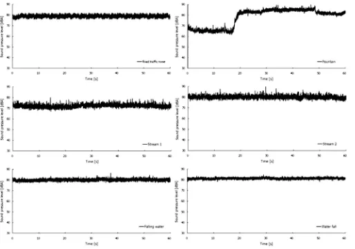
2.2 Temporal Characteristics of Water Sounds

In the present study, it was assumed that road traffic noise was stationary sound according to the classifica-tion of environmental noises outlined in the ISO 1996-116 to simply investigate the masking effect of water sounds. Thus, one-minute recording of water

sound with continuous sound levels was extracted from the selected recordings without road traffic near-by. Figure 3 represents the temporal characteristics of road traffic and water sounds recorded for one minute using a binaural microphone. Similarly, sounds from streams, falling water, and waterfalls demonstrated continuous sound pressure levels. However, water sounds from fountains had different temporal characteristics, with sound pressure levels that varied with the operation cycle of the fountain.

The sound pressure levels of road traffic noise and five water sounds were analyzed in terms ofL10,L50and

L90 and A-weighted equivalent sound pressure levels

共LAeq,1min兲, because the equivalent sound pressure level is not enough to explain sounds that vary over time, such as fountain sounds. L10, L50 and L90 describe the level

exceeded for 10, 50, and 90% of the measuring period. These variables are useful for investigating the differences between water sounds with various temporal characteris-tics. The analysis results of road traffic and water sounds are listed in Table 1.

TheLAeq,1mof water sounds ranged from 72 to 82 dB. The fountain exhibited the highest level of sound pressure and the stream exhibited the lowest. As for water sounds

from streams, falling water, and waterfalls, no differences among the level indices were found. The sound level of the waterfall was 81 dB in terms ofLAeq,1mand other level indices such asL10,L50, andL90were similar, remaining

in the range of 79 to 80 dB. TheLAeq,1m,L10, andL50of

the fountain were similar to those of other water sounds, but L90 dramatically decreased to 65 dB because the

water levels in the fountain fluctuated according to the operation cycle.

2.3 Spectral Characteristics of Water Sounds

The sound pressure levels of road traffic noise and five water sounds are plotted as functions of frequency in Fig. 4, where, for example, F indicates the fountain, and S, FW, and W represent streams, falling water, and waterfalls, respectively. All sound stimuli were set to 75 dB for A-weighted equivalent sound pressure levels. The black column indicates the spectral characteristics of road traffic noise and shows relatively strong energy at low frequencies from 63 to 250 Hz. Among the water sounds, S1 and FW showed slightly more energy than did other water sounds at low frequencies. Thus, it was expected that S1 and FW would be more effective for masking road traffic noise with high sound pressure levels at low frequencies. At mid-frequencies, all water sounds had similar spectral characteristics, but S1 and FW showed much higher sound pressure levels than others at 8 kHz.

3 EXPERIMENT I

Recorded water sounds from different water features represented similar frequency spectra, and none contained any dominant tonal components. In addition, road traffic noises were characterized by a similar spectrum as water sounds. Hence, it was hypothesized that water sounds may be used to mask road traffic noise in urban spaces. In the present study, two labora-tory experiments (Experiment I and II) were designed to examine the proper S/N ratio between water sounds and road traffic noises.

3.1 Procedure

Auditory experiment I was carried out to determine the perceptual difference in the S/N ratio between water sounds and road traffic noise, to be applied to Experi-ment II to evaluate subject preferences for water sounds with different S/N ratios. An auditory experi-ment with two-alternative force choice (2AFC) method was conducted to investigate the just-noticeable differ-ence (JND) of the stimuli17. Each pair of stimuli consisted of a standard stimulus and a comparison stimulus, which were randomized. Road traffic noises were considered standard stimuli, and three types of waster sounds (F, S1, FW) were considered comparison stimuli in this study. The sound pressure levels (A-weighted equivalent sound pressure levels for 10 s, LAeq,10 s) of road traffic noise were fixed at 55 or 75 dBA,

corresponding to the noise exposure of most urban spaces13. When the SPL of road traffic noise was fixed at 55 or 75 dBA, the SPLs共LAeq,10 s兲of water sounds varied

from 49 to 61 dBA and 69 to 81 dBA, respectively, with a step of 1 dB. Therefore, auditory experiment consisted of two sessions; SPL of comparison stimuli were smaller than standard stimulus in the first session, and those were larger than standard stimulus in the second session. Sound pressure levels for stimuli presented to the subjects were set using a head and torso simulator (Brüel & Kjær, Type 4100). The spectral characteristics of the water sounds were not modified for the experiments, but their levels were adjusted. During experiments, subjects

Table 1—Equivalent and percentile sound pressure levels for road traffic and water sounds [dBA] (F; fountain, S; stream, FW; falling water, and W; waterfall).

L_Aeq L₁₀ L₅₀ L₉₀

Road traffic noise 78 79 78 78

F 82 85 82 65

S1 72 73 72 71

Water sounds S2 80 81 80 79

FW 80 80 80 79

W 81 81 81 80

were asked to select the louder stimulus of each pair when the signals were played back to them through headphones (Sennheiser, HD 600). The duration of the stimuli, which consisted of two repeated sounds, was about 10 s, and the inter-stimulus interval (ISI) was set at 1 s. Each pair of stimuli was presented in a random order, separated by an interval of 3 s.

Twenty subjects, 11 males and 9 females between the ages of 22- and 32-years-old, participated in Experi-ment I. Before the experiExperi-ment, the hearing threshold level of the participants was tested via an audiometer (Rion, AA-77) to confirm that all participants had normal hearing. The experiments were conducted in a testing booth共4⫻3 m兲in which the background noise level was approximately 25 dBA.

3.2 Results

Figure 5 represents the results of Experiment I, in which road traffic noise levels were fixed at 55 and 75 dBA. The abscissa represents the difference in S/N ratio between water sounds and road traffic noise. The

ordinate indicates the percentage of correct answers, P(C) [%], given when subjects were asked to identify the louder stimulus. The regression lines obtained from probit analy-sis were plotted in Fig 5. More than 75% of the subjects correctly identified differences in S/N ratio of approxi-mately 3 dB when road traffic noises were presented at 55 and at 75 dBA. The response in the left half (SPL of the water sounds is smaller than that of the road traffic noise) showed the similar tendency to the response in the right half,

4 EXPERIMENT II

4.1 Procedure

In order to identify the optimal S/N ratio between water sounds and road traffic noise to successfully mask the latter with the former, evaluations of subject preference were performed by presenting various water sounds with different sound pressure levels. Sound masking considered in the present study is simulta-neous masking, in which the signal is presented at the same time as the masker, and non-simultaneous masking such as forward or backward masking has not been investigated. Various water sounds (masker) and road traffic noise (maskee) were presented to the subjects simultaneously, then it was investigated whether the masker produces a significant amount of activity and the activity generated by the maskee may be detectable in terms of preference.

An outline of Experiment II is shown in Table 2. The road traffic noise levels were fixed at 55 and 75 dBA 共L_{Aeq,20 s}兲 while the SPLs共L_{Aeq,20 s}兲of the water sounds were varied, for a total of five S/N ratios from −6 to +6 with a step of 3 dB, as derived from Experiment I. Thus, the SPLs of water sounds as presented ranged from 49 to 61 dBA and from 69 to 81 dBA, respectively, for cases including road traffic noise presented at 55 and 75 dBA. Sound pressure levels of combined signal consisting of road traffic noises and the water sounds ranged from 56 to 62 dBA and from 76 to 82 dBA, respectively when the road traffic noise levels were fixed at 55 and 75 dBA. In Experiment II, five water sounds, F, S1, S2, FW, and W were presented as stimuli.

Fig. 5—Results of Experiment I: (a) road traffic noise of 55 dBA and (b) road traffic noise of 75 dBA.

Table 2—Outline of Experiment II.

Road traffic noise

Water sounds

55 dBA 49, 52, 55, 58, and 61 dBA (S/N ratio: −6, −3, 0, +3, and +6 dB)

Paired comparison tests were performed for stimuli (road traffic noise with water sounds) with changes in the S/N ratio. The same 20 subjects who participated in Experiment I also participated in Experiment II. The duration of each stimulus was 20 s with inter-stimulus interval of 0.5 s. The subjects were asked to respond to the following question, “Which stimulus would be more preferable if you were exposed to it in an urban space?” The stimuli were presented to subjects through headphones (Sennheiser, HD 600) in the same manner as in Experiment I.

4.2 Results

The scale values of preferences were calculated using data collected during the auditory experiment II by applying the law of comparative judgment (Thurst-one’s case V)18. Subjects who were able to produce consistent evaluations within a 95% confidence interval (19 out of 20) passed a consistency test. The results of Experiment II indicated that there was significant 共p ⬍0.05兲 agreement among subjects. The results of this experiment are plotted in Fig. 6. Figure 6(a) represents the results in which road traffic noise was presented at 55 dBA, and Fig. 6(b) indicates the results in which road

traffic noise was presented at 75 dBA. The ordinate of each figure shows the scale value of preference, with larger values indicating greater preference, and the abscissa indicates the S/N ratio between the water sounds and road traffic noise.

As shown in the Fig. 6(a), water sounds presented at a S/N ratio of −3 dB were most preferred for all five cases with different S/N ratios when the road traffic noise level was fixed at 55 dBA. And scale values of preference decreased with increasing of level difference between water sounds and road traffic noise. Perhaps this is because the sound pressure levels of road traffic noise combined with the water sounds increased by around 1 to 7 dB, and this led to increment of negative percep-tion of noise such as annoyance and disturbance. However, the subjects preferred the sounds with S/N ratio of −3 dB more than those with S/N ratio of −6 dB showing the lowest sound pressure level. Subjects expressed greater preference for S1 and FW than for the other water sounds, F, S2, and W. This might be because S1 and FW had more energy at low frequencies than other water sounds, suggesting that the spectral characteristics as well as the SPLs of water sounds affect the sound masking of road traffic noise when water sounds are used. A similar pattern was observed when the SPL of road traffic noise was set at 75 dBA. Subjects preferred all five water sound stimuli when the SPL of water sounds was 3 dB lower than that of the road traffic noise. S1 and FW were the most highly preferred water sounds, and S1 showed positive scale values for every case with changes of S/N ratio. Unlike S1, the scale values for F and W were negative and showed almost constant values for every case. This indicates that the sounds of the fountain and waterfall were not effective for masking road traffic noise presented at 75 dBA. The findings from the auditory experiment II expand Brown and Rutherford’s study11 indicating that the S/N ratio of −3 dB produces the highest preference in the zone of influence.

5 CONCLUSIONS

In the present study, the characteristics temporal and spectral aspects of water sounds were analyzed and experiments were carried out to clarify the perceptual differences in the sound pressure levels of water sounds when presented with road traffic noise and to determine the proper S/N ratio between water sounds and road traffic noise for enhancing the perception of urban soundscape. The main findings are:

• The perceptual difference of the sound pressure level of water sounds was determined to be around 3 dB in terms ofLAeq,10 s.

• Water sounds with an S/N ratio of −3 dB were most preferred when road traffic noise levels were fixed at 55 and 75 dBA.

• Sounds from streams and falling water that were characterized by higher energy at low fre-quencies were the most effective for masking road traffic noise.

In the future, the psychoacoustical aspects of water sounds and the visual effects of water images on the preference will be considered in order to propose better design guidelines for water features in urban sound-scape.

6 ACKNOWLEDGMENTS

This work was supported by a National Research Foundation of Korea Grant funded by the Korean Government (2009-0076495).

7 REFERENCES

1. “First National Bank Plaza: A pilot study in post construction evaluation”, Champaign-Urbana: University of Illinois, Depart-ment of Landscape Architecture, (1975).

2. T. Banerjee and L. Anastasia, “Private production of downtown public open spaces: Experiences of Los Angeles and San Fran-cisco”, Los Angeles: University of Southern California, School of Urban and Regional Planning, (1992).

3. S. Kaplan, “Aesthetics, affect, and cognition—environmental preference from an evolutionary perspective”,Environ. Behav.,

19, 3–32, (1987).

4. C. C. Marcus and C. Francis,People places: Design guidelines for urban open space, John Wiley & Sons, (1998).

5. W. Yang and J. Kang, “Soundscape and sound preferences in urban squares: A case study in Sheffield”,Journal of Urban De-sign, 10, 61–80, (2005).

6. W. Yang and J. Kang, “Acoustic comfort evaluation in urban open public spaces”,Appl. Acoust., 66, 211–229, (2005). 7. R. Pheasant, K. Horoshenkov and G. Watts, “The acoustic and

visual factors influencing the construction of tranquil spaces in urban and rural environments”,J. Acoust. Soc. Am., 123, 1446– 1457, (2008).

8. E. Zwicker and H. Fastl,Psychoacoustics: Facts and Models, Springer, (1999).

9. A. C. C. Warnock, “Acoustical privacy in the landscaped of-fice”,J. Acoust. Soc. Am., 53, 1535–1543, (1973).

10. E. Lewis, D. Sykes and P. Lemieux, “Using a web-based test to measure the impact of noise on knowledge workers’ productiv-ity”, Human Factors and Ergonomics Society 47th Annual Meeting, Denver, USA, (2003).

11. A. L. Brown and S. Rutherford, “Using the sound of water in the city”,Landscape Australia, 2, 103–107, (1994).

12. G. Watts, R. Pheasant, K. Horoshenkov and L. Ragonesi, “Mea-surement and subjective assessment of water generated sounds”,Acta Acust., 95, 1032–1039, (2009).

13. J. Y. Jeon, P. J. Lee, J. You and J. Kang, “Perceptual assessment of urban soundscape quality with combined noise sources and water sounds”,J. Acoust. Soc. Am., 127, 1357–1366, (2010). 14. F. Hooimeijer and W. T. Vrijthoff,More urban water: Design

and management of Dutch water cities, Taylor & Francis, (2008).

15. S. Dewar, “Water features in public places-human responses”,

Grad. Dip. Landscape and Architecture thesis, Queensland Uni-versity of Technology, (1990).

16.Acoustics—Description, measurement and assessment of envi-ronmental noise—Part 1; Basic quantities and assessment pro-cedures, International Standard ISO 1966: 2003, International Organization for Standardization, Geneva, Switzerland, (2003). 17. J. You and J. Y. Jeon, “Just noticeable difference of sound qual-ity metrics of refrigerator noise”, Noise Control Eng. J., 56, 414–424, (2008).