Accident Analysis and Prevention: Course Notes 1987/88

This is a repository copy of Accident Analysis and Prevention: Course Notes 1987/88. White Rose Research Online URL for this paper:

http://eprints.whiterose.ac.uk/2285/

Monograph:

Nicholson, A.J. and Tight, M.R. (1989) Accident Analysis and Prevention: Course Notes 1987/88. Working Paper. Institute of Transport Studies, University of Leeds , Leeds, UK. Working Paper 272

[email protected] https://eprints.whiterose.ac.uk/

Reuse

See Attached

Takedown

If you consider content in White Rose Research Online to be in breach of UK law, please notify us by

White Rose Research Online

http://eprints.whiterose.ac.uk/

Institute of Transport Studies

University of Leeds

This is an ITS Working Paper produced and published by the University of Leeds. ITS Working Papers are intended to provide information and encourage discussion on a topic in advance of formal publication. They represent only the views of the authors, and do not necessarily reflect the views or approval of the sponsors.

White Rose Repository URL for this paper: http://eprints.whiterose.ac.uk/2285/

Published paper

Nicholson, A.J., Tight, M.R. (1989) Accident Analysis and Prevention: Course Notes 1987/88. Institute of Transport Studies, University of Leeds. Working Paper 272

Working Paper 272

July 1989

ACCIDENT ANALYSIS AND PREVENTION: COURSE NOTES 1987188

A.

J.

Nicholson

and

PREFACE

This report consists of the notes from a series of lectures given by the authors for a course entitled Accident Analysis and Prevention. The course

took

place during the second term of a one year Masters degree course in Transport Planning and Engineering run by the Institute for Transport Studies and the Department of Civil Engineering a t the University of Leeds. The course consisted of 18 lectures of

which 16 are reported on in this document (the remaining two, on Human Factors, are not reported on in this document

as

no notes were provided). Each lecture represents one chapter of this document, except in two instances where two lectures are covered in one chapter (Chapters 10 and 14). The course first took place in

1988, and at the date of publication has been run for a second time. This report

TABLE

OF

CONTENTS

PREFACE

. . .

1.INTRODUCTION 1

1.1. BASIC DEFTNITIONS

. . .

1

1.2. THE ACCIDENT SITUATION IN GREAT BRITAIN

. . .

2

1.3. INTERNATIONAL COMPARISONS

. . .

2

.

. . .

2 THE DRIVER. THE VEHICLE AND THE ROAD ENVIRONMENT 7 2.1. INTRODUCTION

. . .

7

2.2.THEUSER

. . .

7

2.3. THE VEHICLE

. . .

10

. . . . . .

2.4. THE ROAD ENVIRONMENT 12 2.5. PERCEPTION-REACTION

. . .

13

. . .

3

.

A COMPREHENSIVE STRATEGY FOR ACCIDENT COST REDUCTION 15

. . .

3.1.ACCIDENTFACTORS 15 . . . 3.2. POTENTIAL SAVINGS

. . .

16

-"

3.3. ACCIDENT INVESTIGATION AND PREVENTION

. . .

18

3.4. OBJECTIVES AND TARGETS

. . .

19

3.5. FINANCIAL AND STAFF RESOURCES

. . .

~ 19 ..

3.6. DATA-BASE REQUIREMENT

. . .

20

3.7. ANALYSIS AND SYNTHESIS

. . .

22

3.8. IMPLEMENTATION AND MONITORING

. . .

24

.

. . .

4 ACCIDENTS. VEHICLES. POPULATION. SMEED TYPE ANALYSIS 25 4.1.PROBLEMS

. . .

25

4.2. METHODS OF MAKING INTERNATIONAL COMPARISONS

. . .

25

4.3. THE SMEED EQUATION

. . .

27

4.4. OTHER TECHNIQUES

. . .

28

. . .

5

.

ACCIDENTS. EXPOSURE. RISK AND TRAFFIC FLOWS

. . .

5.1. INTRODUCTION 5.2. MODEL ESTIMATION

. . .

31

5;3

.

LINK

EXPOSURE FUNCTION

. . .

32 . .

. . .

5.4. INTERSECTION EXPOSURE FUNCTION

6

.

ACCIDENT OCCURRENCE AS A STOCHASTIC PROCESS

. . .

. .

. . .

6.1. INTRODUCTION

. . .

~ ~ ~ ~ ~ ~

6.2. ANALYSIS OF TEMPORAL VARIATIONS

. . .

6.3. ANALYSIS OF SPATIAL VARIATIONS

. . .

. . .

7.ACCIDENTDATA-BASE

7.1. THE ACCIDENT REPORTING SYSTEM

. . .

. . .

7.2. SYSTEM EFFICIENCY

7.3. DATA MANAGEMENT

. . .

7.4. DEFICIENCIES IN THE DATA-BASE

. . .

8

.

IDENTIFICATION OF HAZARDOUS SITES. ROUTES AND AREAS

. . .

. . .

8.1. INTRODUCTION

8.2. IDENTIFICATION OF HAZARDOUS SITES

. . .

8.3. IDENTIFICATION OF HAZARDOUS ROUTES

. . .

8.4. IDENTIFICATION OF HAZARDOUS AREAS

. . .

:

. .

8.6. EFFICIENCY OF IDENTIFICATION PROCEDURES

. . .

68

8.7. RANKING OF LOCATIONS FOR TREATMENT

. . .

71

9

.

PROBLEM DIAGNOSIS VIA ANALYSIS OF' ACCIDENT DATA 9.1. INTRODUCTION

. . .

. . .

9.2. BASIC DATA 9.3. DATA PRESENTATION AND ANALYSIS

. . .

9.4. HUMAN FACTORS

. . .

9.5. IN-DEPTH ANALYSIS

. . .

9.6. AREA WIDE ANALYSIS

. . .

TRAFFIC CONFLICTS TECHNIQUES

. . .

10.1. INTRODUCTION

. . .

10.2. DEFINITION OF A TRAFFIC CONFLICT

. . .

. . .

10.3. SOME TRAFFIC CONFLICT PROCEDURES 10.4. PROCEDURES USING SPACE-TIME TRAJECTORIES 10.5. STUDY DURATION

. . .

. . .

10.6. OBSERVER RELIABILITY 10.7. VALIDITY OF THE TRAFFIC CONFLICTS TECHNIQI 10.8. APPLICATION

. . .

ROAD ENVIRONMENT FACTORS

. . .

98

11.1. INTRODUCTION

. . .

98

11.2. STUDY METHOD

. . .

99

11.3. SURFACE CONDITIONS

. . .

100

11.4. ROAD LIGHTING

. . .

103

11.5. CROSS-SECTION CHARACTERISTICS

. . .

105

11.6. ALIGNMENT CHARACTERISTICS

. . .

108

11.7. INTERSECTION CONTROL AND LAYOUT

. . .

111

11.8.

LAND

USE

. . .

112

11.9. CONCLUSION

. . .

113

12

.

PEDESTRIAN SAFETY

. . .

114

12.1. ACCIDENTS

. . .

114

. . .

12.2.EXPOSURE 117 12.3. PEDESTRIAN BEHAVIOUR

. . .

118

12.4. PREVENTION OF PEDESTRIAN ACCIDENTS

. . .

120

. . .

VALUATIONSTUDIES 13.1. INTRODUCTION

. . .

13.2. CHOICE OF PERFORMANCE INDICATOR

. . .

13.3. CHOICE OF OBSERVATION PERIOD

. . .

13.4. CHOICE OF CONTROL SITE

. . .

13.5. REGRESSION.TO.THE.MEAN, BIAS.BY.SELECTION, AND

. . .

ACCIDENT MIGRATION 13.6. RISK COMPENSATION AND ACCIDENT MIGRATION

. . .

13.7. DISCUSSION

. . .

14

.

ECONOMIC EVALUATION

. . .

135

14.1. INTRODUCTION

. . .

135

14.2. TREATMENT SELECTION PROCEDURES

. . .

135

14.3. THE COST OF ACCIDENTS

. . .

137

14.4. CONCLUSION

. . .

143

REFERENCES

. . .

145

-

1.

INTRODUCTION

1.1. BASIC DEFINITIONS

Accident

-

an event occurring on a public roadway or footway, and involving a vehicle and personal injury or property damage

-

injury accidents and non-injury (property -damage-only)

accidents

-

generally, only injury accidents must be reported and often accident statistics relate to injury accidents only

Injury

-

fatal, if person dies within specified time of Severity event (30 days for Great Britain)

-

serious, if person is either detained in hospital as "in-patient" or suffers fractures, concussion, internal injuries, crushings, severe cuts and lacerations, severe shock, or death after specified time limit

-

_{minor (slight), if not fatal or serious (e.g. sprain, bruise, minor} cuts, minor shock).

Accident

-

based on severity of injury to most severely injured participant Severity

Participants

-

generally classified according to whether driver, passenger, rider (of pedal cycle, motor cycle, or animal) or pedestrian

-

"road user" incorporates all classes of participants

Vehicles

-

generally classified as cars, goods vehicles (heavy or light), two-wheel motor vehicles (motor scooters and motor cycles) and pedal cycles

Accident

-

generally classified according to whether in a

Location

(i) "built-up" or urban area; on roads with permanent speed

limit of 40 mph or less (say)

(ii) "non built-up" or rural area; on roads with permanent speed limit greater than 40 mph (say)

Accident time

-

generally classified according to whether in

(i) day-time (e.g. 30 min. before sunrise to 30 min. after sunset)

1.2. THE ACCIDENT SITUATION IN GREAT BRnAIN

Described in the documents (published annually by the Department of Transport) (1) Road Accidents Great Britain

(2) Road Accident Statistics English Regions (3) Road Accidents: Scotland

(4) Road Accidents: Wales

Items 2-4 supplement item 1, and concentrate on data of most use to traffic engineers, planners and administrators in local and regional government. All four documents are based on analysis of data in the accident report form (Stats 19). The situation in Great Britain has been changing with time, with changes in factors such as population, the number of vehicles, and vehicle use (see Figure 1).

It should be noted that aggregate statistics (for all road users) masks the variability that exists between road users (see Figure 2). Further disaggregation of the data

for each class of user, according to age (say), reveals that there is considerable variation between groups within the same user class (see Figure 3).

1.3. INTERNATIONAL. COMPARISONS

Comparisons of accident situations in different countries is &aught with danger, due to

(1) variations in definitions in injury severity; for instance, the specified time limit for a fatal injury varies from 3 days (Greece, Austria)

to

12 months (Canada), with 30 days being most common.

(2) variations in accident reporting requirements.

(3) variations in the reporting rate; the reporting rate may vary considerably according to the accident severity and the class of participant.

A study of the time interval between the accident and death, for fatal accidents in Great Britain in 1985, has revealed that

(1) death occurs more quickly for non built-up roads (68%, 86%, 95%, 99% and 100% within 1 hour, 12 hours, 5 days, 15 days and 23 days, respectively)

(2) death occurs less quickly for built-up roads (53%, 7356, 90%, 97% and 100% within 1 hour, 12 hours, 5 days, 15 days and 25 days, respectively)

Hence, a 30 day period seems appropriate, and using such information, the number of deaths for countries using a different period can be adjusted.

Comparisons between countries are generally in terms of deaths, injuries or accidents per head of population, vehicle or vehicle-kilometres (a measure of vehicle usage). Some such rates are not an ideal basis for comparison (see Andreassen, Traffic Engineering and Control, November 1985), but there are practical d%culties obtaining some data in some countries. Table 1 shows the results of a recent

international comparison.

-

I-a &I-&

1.

I n t e r n a t i o n a l c o m p a r i s o n s of road d e a t h s : n u m b e r , and r a t e s for d i f f e r e n t r o a d users:

by s e l e c t e d c o u n t r i e s : 1985

Nunber o f Motor v e h i c l e s Road deaths Road deaths Car user Pedestrian road deaths1 per 1,000 per 100,000 per 10,000 deaths per deaths per

population population motor 100 m i l l i o n 100.000

vehicles car kilometres p a p l a t i o n

England

Ua 1 es Scotland Great B r i t a i n Northern Ireland United Kingdom

Belgiun 1,801 415 18.3 4.4 2.7' 7 d 3.3

Dermark 772 381 15.1 4.0 1 . 2 ~ ~ 2.5

Federal Republic o f Germany 8,400 493 13.8 2.8 1.3 2.9

France 11,387 510 20.7 4.lZb 3 . 1 ~ ' 3.1

Greece 1 , 9 0 8 ~ 206 19.3' 10.1 .

.

4.92

I r i s h Republic I t a l y

Luxenbwrg Netherlands Portugal Spain A u s t r i a Czechoslovakia Finland

German Democratic Reprblic H w a r y

Norway Poland Sueden Suitzerland Yugoslavia

A u s t r a l i a 2.942

-.

18.7 3.2

.

. _3.4

Camda 3,9142 5 9 1 ' ~ 1 5 . 6 ' ~ 2.6'

. .

2.2'

Japan 12,039 400 10.0 2.5 .

.

2.9

New Zealand 747 607 22.7 3.7

. .

_3.8

U n i t e d States o f America 43,795 727? 18.3 2.6' l . l C _2.8

In accordance u i t h t h e camwxlly agreed i n t e r n a t i o n a l d e f i n i t i o n , most c w n t r i e s d e f i n e a f a t a l i t y as being due t o a road accident if death occurs uithin 30 days of the accident. The o f f i c i a l road accident s t a t i s t i c s of sane c w n t r i e s houever, L i m i t t h e f a t a l i t i e s t o those occurring u i t h i n shorter p e r i c d s a f t e r t h e accident. Nunbers of deaths and death r a t e s i n the above t a b l e have been adjusted according t o t h e factors used by the E c o m i c Comnission f o r Europe and t h e European Conference of M i n i s t e r s of Transport, t o represent standardised 30-day

deaths: France ( 6 days) + 9%; I t a l y ( 7 days) +7X; Greece, A u s t r i a (3 days) +12X; Spain, Japan (24 hours) +3OX;

Canada. Suitzerland (1 year)

-

5%; Portugal Cat t h e scene) +35X

See a r t i c l e 15, which analyses t h e time t o d i e a f t e r a road accident. This a r t i c l e estimates the percentage of deaths occurring u i t h i n a s p e c i f i e d nurhr of days a f t e r a road accident. The r e s u l t s obtained from t h i s study may a t s m stage influence t h e adjustment f a c t o r s used i n t h i s t a b l e t o standardise road accident deaths to t h e agreed i n t e r n a t i o n a l d e f i n i t i o n o f death w i t h i n 30 days

1984 1983

'

1981

excluding mopeds excluding l o r r i e s

'

n a t i o n a l s ' v e h i c l e s o n l y

t r a f f i c on s t a t e roads o n l y i n c l u d i n g t r a f f i c on p r i v a t e roads

"

i n c l u d i n g n a t i o n a l s ' cars abroad excluding a l l two wheel motor vehicles i n t e r c i t y t r a n s p c r t

FI k v R L

1: Population, vehicles licensed, accidents, traffic and

casualities:

1926-1986

(Logarithmic Scale)

Population and Number of Vehicles

IMillions) Accidents and _IThourandrl Casualties

1926 1930 1935 1940 1945 1950 1955 1960 1965 1970 1975 1980 1985 1990

2.

THE

DRIVER,

THE VEHICLE AND

THE

ROAD

ENVIRONMENT

2.1. INTRODUCTION

The driver-vehicle-road environment system is rather complex. It is convenient to consider it as 3 interacting sub-systems:

3

"'

""'

"\,

the v e h i c l e the road environment

Accidents arise from the interaction of 2 or 3 of the sub-systems. Traffic engineers should have a clear understanding of

(1) the elements of each sub-system, and

(2) how each sub-system interacts with the other two.

2.2. THE USER

The elements of the user sub-system are either phvsioloeical or psvchological, and include

Phvsiological Psvchological

the nervous system motivation

vision intelligence

hearing learninglexperience

stability sensations emotion other senses (eg touch, smell) maturity

modifiers (eg fatigue, drugs) conditioninghabits

User behaviour is derived from the interaction of the above human factors amongst themselves, subject to other factors, including those related to the vehicle and road environment sub-systems

Nervous Svstem

The central part of the nervous system contains about 2000 million cells. Different parts of the brain are concerned primarily with different functions, there being single master central control i.e. it is a system maintained by the effectiveness of intercommunicating parts.

The basic unit of the nervous system is the neurone, of which there are two types (1)

motor

(for muscle control

-

messages h m brain)

vision

The eye is the primarv sensorv organ for road users. The visual field for normal sight is approximately

180° horizontally 145' vertically There are various cones of vision

(1) cone of readina vision

-

2%" horizontally and2S0 vertically (2) cone of acute vision

-

6" horizontally and 4" vertically (3) cone of sensitive vision

-

20" horizontally and 13" vertically

The above cones constitute the central field of vision, and the eye can detect the details of obiects within the central field.

As well, there is the remainder of the visual field, giving rise to peripheral vision. Objects within the peripheral limits (180° horizontally and 145" vertically) can be detected readily, if those objects are sufficiently stimulating.

For

example, a child moving from the footpath may be initially detected by peripheral vision, and the driver can shift his gaze, in order to focus upon the point of activity.

Both central and peripheral vision are important to road uses, with peripheral vision being particularly important with regard to meed iudgement and steering.

Visual acuity is the ability to discern details, and an adequate level of visual acuity is required before drivers are licensed. (Snellen visual acuity test)

Vision is afTected by movement. As speed increases, drivers focus on objects further away. As the focal point distance increases, the visual field decreases (i.e. peripheral vision is reduced)

speed focal point distance field of vision

( k d )

(metres)

40 180 100°

Also, as speed increases, concentration increases and detailed scanning is reduced (i.e. the point of focus shifts less).

Linear streaming is the term applied to the linear 'exvansion' of objects in the field of vision. The apparent rate of displacement of objects increases as the object moves away from the centre of the visual field, assuming that the driver is looking in the direction of travel. In the case of linear streaming, moving objects will appear as

marked discontinuities, and will be readily detected.

However, if the driver's eyes are directed away from the direction of movement, then the detection of moving objects is difficult, unless they are within the immediate vicinity of the point of focus. That is, 'vulnerability' increases whenever drivers' eyes are not directed in the direction of movement (e.g. higher accident rates at intersections, where drivers must look for cross-traffic).

-

During driving, the point of fixation will move regularly, and vision is poor during such shifts.

shift time 0.15

-

0.33 sec fixation time 1 0.10

-

0.30 sec

The frequency of shifts will depend upon the driving situation. Also, blinking occurs about 5 times per minute (if lower, then fatigue results) and vision is lost for about

0.3 sec during each blink.

Driver vision can be reduced massively by glare, especially glare from approaching headlights

-

perhaps to only about 30% of the no-glare vision. Also, changes in the level of light cause the pupils to either contract or dilate. The contraction time is fairly short, but the dilation time can be considerable.

about 2% sec for 90% contraction about 200 sec for 90% dilation

Therefore, a change from light to dark (e.g. upon entering a tunnel) is a critical time for drivers.

Hearing

The sense of hearing is generally much less important to road users than is vision, with pedestrians probably relying more upon hearing than other road users.

However, the sound of tyres on pavements, wind, engine noise, horns and other traffic noise are useful to road users.

Stabilitv sensations and other senses

The vestibular o r a s (located within the inner ear) are sensitive to

acceleration/deceleration and orientation, and many of the vehicle control

adjustments are based upon the information relating to balance and stability.

Also, drivers can detect f i e or overheating engineslbrakes via the olfactorv senses (i.e. by smell). The sense of

touch

enables the detection of vibrations.

Psvcholorrical factors

A driver receives various stimuli (e.g. visual, auditory, vestibular) while driving. The response depends upon:

(1) the nature of the stimulus

(2) the strength of the stimulus

(3) the psvcholorrical state of the driver, as defined by the psychological

factors listed above.

Some examples of how psychological factors affect driver behaviour are:

(1) the purpose of a trip might be such that the driver is strongly motivated to reach the destination as quickly as possible;

(2) a driver may be disturbed because of an event prior to driving and may be less attentive than usual;

(3) young/immature drivers tend to take greater risks while driving;

(4) a conditional response (or habit) when approaching particular intersections might be to assume the right-of-way and maintain speed.

It is widely believed that there is an optimum amount of driver anxiety

-

too little or too much is related to a deterioration in driving ability. Likewise, fits of depression or elation are not conducive to good driving, there being an 'optimal' medium emotional state. A driver's response to frustration (e.g. unnecessary delay a t signalised intersections) depends upon the psychological state a t that time.

2.3.

THE

VEHLCLE

Fortunately, the vehicle has less variable characteristics than road users (there are fewer manufadurers of vehicles than road users). Also, there is a greater amount of legislative control over the tkatures of vehicles than of road users, for instance:

(1) limits upon overall weight, size and performance; (2) minimum requirements for brakes, lights etc.

The more important vehicle factors are: (1) visibility

(2) lighting

(3) warning and instrument systems (4) brakes

(5) stability

( 6 ) size and weight

(7) power. Visibility

Because of pillars, roof and bonnets, the driver's field of view is restricted somewhat. Typical fields of view are (for saloon cars)

(1) forward:

58" to left and 31.5" to right

-

horizontally 12.2" upwards and 9.3" downwards

-

vertically

(2) rear:

28.5" horizontally via mirror 3S0 horizontally directly 5.7" vertically

The pillars can be critical, obscuring the driver's view of pedestrians and cyclists

-

typically, the obstructions are

about 4" for right h n t pillar and 2" for left front pillar

The presence of a passenger adjacent to driver can reduce the view to the side. Clearly, the vehicle body restricts the driver's view, which is dependent upon the eye position of the driver relative to the body of the car.

Also, the height of the driver's eye relative to the ground is of significance when determining how far ahead the driver can see (especially on vertical curves). The driver's eye height has been decreasing in recent times.

Lighting

Vehicle lighting has two main purposes:

(1) to define the vehicle to external viewers;

(2) to provide an illuminated field of view for the driver. The illuminated field of view can vary considerably, depending upon:

(1) vehicle and lamp type

(2) whether beams dipped or not (3) climaticlweather conditions (4) presence of opposing vehicle. Vehicle Warning and Instrument Svstems

The style and positioning of instruments varies between vehicles, with driver vision being lost for 1-3 seconds each time the instruments are monitored.

Brakes

With efficient modern braking systems, the onset of skidding generally limits the deceleration capability of vehicles. Typical rates of deceleration and thresholds are:

(1) initial slowing down: 1-3 m/s2

(2) final braking to stop: up to 3.5 mls2

(3) emergency stops : between 6 and 10 m/s2

The locking of wheels in a non-symmetric manner (with respect to the direction of travel) may induce vehicle swerving (i.e. a loss of control).

Stability

The suspension characteristics of vehicles vary, giving rise to varying degrees of understeer (desirable) and oversteer (undesirable).

The ability of a vehicle to accelerate depends upon its weight (and vehicle size) and the power (and engine size and performance). Typical acceleration rates in normal use are

(1) medium cars 3-8 km/h/s (0.85

-

2.20 m/s2) (2) sports cars 12-16 km/h/s (0.33

-

4.50 d s 2 ) (3) commercial vehicles 0.75-2 kmMs (0.21

-

0.56 m/s2)

2.4. THE ROAD ENVIRONMENT

There are five major components of the road environment:

(1) the traffic stream

-

flow rate, flow composition, traffic speed;

(2) the road design

-

alignment, road surface, frequency and type of intersections;

(3) the land use adjacent to road

-

urban, rural, commercial etc. (4) the legislation and enforcement measures;

(5) climaticlweather conditions, lighting.

The road environment places demands upon drivers and their vehicles. The demand upon a driver varies with time and space, because the road environment changes in time and space.

While driving, one does not maintain a constant level of alertness. Rather, there are periods of high alertness (or concentration) separated by periods of relative relaxation.

The ideaUperfect driver will ensure a matching of his level of alertness with the demands imposed by the road environment. Drivers are not perfect and there are instances where the demands upon a driver are not met, because:

(1) the driver responded too slowly to a changing demand;

(2) the demand exceeded the driveis capability, even when a t a peak alertness.

In such situations, an accident occur; the driver may manage to recover and avoid an accident.

As well as placing demands upon drivers, the road environment can affect the driver's ability to function. For instance:

weather and lighting conditions affect the physiological functions, either directly (e.g. excessive heat can induce fatigue, with consequent deterioration of physiological functions) or indirectly (e.g. effects upon psychological state of

a

driver);

2.5.

PERCEPTION-REACTION

At the heart of the user-vehicle-road environment interaction is the process of perception.

Recognising and responding to a stimulus is more complex than simply receiving sensory information (e.g. visual information). Once a stimulus

has

been detected (e.g. an object

has

been seen), the road user must interpret the information. The interpretation results from a complex association between the conscious ~hvsical and unconscious ~svchological world.

A stimulus will only be registered by the brain if it exceeds a certain threshold level. There are two major reasons why

a

stimulus is not registered:

(1) The activity level of the brain (known as the level of arousal) varies, from deep coma through relaxed wakefulness to extreme excitement. High levels of arousal (induced by strong stimuli or superposition of several stimuli) are normally followed by a period of low response (or recuperation). Regular stimuli of similar type and magnitude, may impose rhythmic sensations upon the brain, leading to a hwnotic state (e.g. regularly spaced service poles a t side of road crossing expansive plain can induce hypnosis).

(2)

There are stronger stimuli competing for attention.

Reaction time is defined as that time which elapses between the reception of an external stimulus and the taking of an appropriate action.

Reaction time necessarily includes perception time. Complex and new situations require more thought and association with past experience, in order to identify an

appropriate action, than do simple or frequently encountered situations (e.g. a red traftic signal). This thinking process is known as intellection.

Intellection does not always follow perception

-

emotion sometimes intervenes, giving rise to irrational decisions/actions. Emotion is a strong, complex mental and physical response to external stimuli. Emotion can exert a powerful effect upon driver behaviour (e.g. irritation at other drivers).

Volition is the exercise of the will and the settlement of deliberation by making a decision, which is actioned.

Traffic engineers are interested in the total time taken, that is the perception- intellection-emotion-volition time (or

=

time). It is also commonly called the ~erception-reaction time.

Consider the following simple sequence of events:

(1) at time

&,

a n obstruction on intended vehicle path becomes visible;

(2) at time

&,

the driver registers the fact that his intended path is obstructed;

(3) the driver thinks about the situation and considers alternative actions, before deciding a t time

t,

to stop;

-

t,

-

intellection time

t,

-

t,

-

volition time

t,

-

t,

-

PIEV time

In the above sequence, emotion appears to have not entered into the process. If the driver determines that the obstruction is a vehicle which should have given way, he may decide to 'teach the other driver

a

lesson' and ram into the obstruction (which may be relatively small).

Most studies of perception-reaction time have been confined to estimating driver brake reaction time (i.e., the t i e taken to perceive the situation, to decide upon applying the brakes, and to commence depressing the brake pedal).

It has been found that brake reaction time depends upon:

(1) whether the stimulus is expected or unexpected;

(2) the strength of the stimulus.

For example, in laboratory tests, the average b.r.t. is 0.4 to 0.5 sec, compared to normal road conditions, where the average b.r.t. is:

0.8 see

-

if brake lights of preceding vehicle functioning

1.7 sec

-

if brake lights of preceding vehicle not functioning

Steering reaction time is shorter than brake reaction time. However, the perception- reaction time for more complex or new situations may be much greater

-

between 2

and 6 seconds.

Finally, it seems that brake reaction time is not correlated with accident frequency.

3.

A COMPREHENSIVE

STRATEGY

FOR ACCIDENT COST REDUCTION

3.1. ACCIDENT FACTORS

During the 1960s and 19708, a number of in-depth investigations of road accidents were undertaken in several countries, with a view to obtaining a better understanding of the factow involved in accidents (the "causes") and the interrelationships between those factors. The results of three of the more notable studies are shown below, with factors having been grouped as "road environment"

(E),

"user"

(U)

or "vehicle"

(V),

or some combination.

E U V EU EV W E W

2.0 76.5 3.0 16.0 0.1 2.0 0.3

UK, 1978-81 (Sabey, 1983)

2.5 65.0 2.5 24.0 0.3 4.5 1.4

UK, 1970-74 (Sabey 6 Staughton, 1975)

3.3 57.1 2.4 26.4 1.2 6.2 2.9

USA, 1972-77 (Treat et al, 1977)

Sinsle (U t E

+

V) 81.5 70.0 62.8

Double (EU

+

EV t W) 18.1 28.8 33.8

Triple (EW) 0.3 1.4 2.9

UK, 1978-81 UK, 1970-74 USA, 1972-77

Note: (1) Substantial difference in study results in the extent of user/environment interaction

Sub-system % of accidents in which involved

UK, 1978-81 UK, 1970-74 USA, 1972-77

Results of studies of accident factors seem to suggest the greatest potential for reducing accidents lies in changing user behaviour.

When a user fails to cope with the road environment, the "cause" may be ascribed to user error. However, changes to the environment so that more users can cope may well be more cost-effective and practicable.

Accident costs can be reduced by: (1) reducing accident freauencv

(2) reducinv iniunr severity

Primarv safetv measures reduce accident hquency

(e.g. improved geometry, relocation of poles) Secondarv safetv measures reduce injury severity

(e.g. seat belts, energy-absorption systems)

3.2. POTENTIAL SAVINGS

Sabey and Taylor (TRRL, 1980) estimated the potential s a v i n ~ s of proven remedial actions, for which there is strong evidence of potential benefits. They estimated, for each remedy individually,

(1) the % reduction in accidents or injuries (x%, say)

(2) the % of accidents or injuries susceptible to reduction by the remedy (y%, say)

POTENTIAL SAVING (%)

Environment

-

Overall

-

20

Geometrical design, especially junction

design and control 10.5

Road surface texture 5.5

Road lighting 3.0

Land use, road design and traffic management

in urban areas 5.0 to 10.0

User

-

Overall

-

33.3

-

Drinking and driving restrictions 10.0 More appropriate speed limits 5.0 Pmaeanda and information UD to 5.0

~nfbr&ment

Education and training

Other (e.g. parking restrictions) Vehicle

-

Overall

Vehicle maintenance

Anti-lock brakes and safetv tvres ) ~ r i m a r v 7.0

Improved motorcycle consI;ic&y . ) a

"

3.5

Seat Belts ) 7.0

Other occupant protection measures ) secondary 5.0 to 10.0

All Measures

-

60

Sabey and Taylor conclude that it is possible to obtain

(1) a 60% reduction in the cost of injury accidents

(2) a 50% reduction in the cost of non-injury accidents (must exclude effects of secondary measures)

A recent review of road safety policy in the

UK

(Department of Transport, 1987) concluded that a reduction

(1) of 30% i n injuries per annum by the year 2000 is reasonable (i.e. 320,000 to 220,000 per annum).

(2) the bulk of the reduction (80% of the 100,000) will be achieved by the "indirect a ~ ~ r o a c h " and only 20% by the "direct approach.

Indirect approach: involves creating an environment in which the scope for the road user to behave in

an

unsafe manner is reduced.

Direct approach: involves inculcating in each road user an understanding of the standards of skill and behaviour conducive to road safety and persuading each user to comply with those standards.

Expected Injury Saving Direct measures

Indirect measures:

(i) vehicle 43,500

(i) safety benefits of highway

improvement schemes 15,000 (iii) safety engineering (especially

accident investigation and

prevention in urban areas) 21,500

3.3. ACCIDENT INVESTIGATION AND PREVENTION

In the UK, each local authority has a statutory obligation (Road Traffic Act, 1984,

9.8) to:

"prepare and carry out a programme of measures designed to promote road safety, and shall have power

to

make contributions to the cost of measures for promoting road safety taken by other authorities or bodies".

To assist local authorities to discharge their statutory obligation,

the

Institution of Highways and Transportation have produced "Highway Safety: Guidelines for Accident Reduction and Prevention" (second edition, 1986).

In the guidelines,

it

is stated that:

"The whole area of accident reduction and prevention endeavour calls for a systematic approach to achieve:

(1) the greatest benefits from minimum cost

(2) to enable past work to be evaluated."

This is tantamount to saying that a "com~rehensive strategy" is required for improving road safety.

Development of a comprehensive strategy will entail the following:

(1) Defining overall objectives and setting quantified targets.

(2) Determining what financial and staff resources are required and ensuring those requirements are met.

(3) Identifying what data is required and ensuring they are available. (4) Establish appropriate procedures for the analysis and interpretation of

the data, and the development of effective remedies and a programme of works.

(5) Implementing that programme and monitoring the effects, checking that the overall objectives and specific targets are being achieved. Non-achievement of targets should result in an analysis of the reasons and either

_-

(i) allocating more resources or revising the data collection, data analysis and/or solution synthesis stages;

(ii) revising objectives andlor targets.

3.4. OaTECTIVES AND TARGETS

The

I H T

guidelines propose the following objectives:

"To reduce the overall number and severity of accidents by road engineering and traffic management through

(i) the application of cost effective measures on existing roads as a basis for accident reduction, and

(ii) the application of safety principles in the provision, improvement and maintenance of roads as a means of accident prevention."

A survey of highway authorities in the UK has revealed that virtually all accept the IHT statement of objectives (Sicock and Smyth, 1985).

The IHT guidelines endorse a 20% saving as a feasible target for accident reduction by low cost engineering measures, as proposed by Sabey and Taylor (1980) and confirmed by the Department of Transport (1987).

3.5. FINANCIAL AND STAFF RESOURCES

Experience in the

UK,

NZ

and elsewhere has revealed that "low cost engineering measures" aimed at accident reduction are very cost-effective, in general. A typical first-year-rate-of-return is 200%

-

300%.

It is now common that a specific financial allocation of funds is made for such work, which is generally the most cost-beneficial of the works undertaken by highwaylroading authorities.

The need for the application of safety principles in roading improvement schemes to reduce delay, etc. must not be forgotten. The budget allocation for the planning, design and implementation of such schemes must allow for "safety checking".

"Low cost engineering measures": the cost of the implementation is low, but the cost of preparatory work is high relative to the implementation cost. Preparatory work is typically 20%

-

50% of the total cost (c.f. 2%

-

5% for other roading improvement schemes).

The preparatory work is time-consuming and requires specialist skills:

"The technique of accident investigation and the design of remedial measures requires specialist engineering expertise of a high order."

The M T recommends the establishment of

a

separate, specialist accident unit, giving

(i) economies of scale

(ii) improved effectiveness through the pooling of expertise

The recommended s t f f i g level is 1 engineer (or highly skilled technician) for every

400

-

1000 injury accidents in the authority's area each year.

The accident unit would be responsible for:

(i) accident investigation and prevention via low cost works (ii) safety checking of other roading improvement works The latter task can readily take 20%

-

25% of staff time.

Appropriate training for new mad safety engineers and technicians is essential. In addition,

it

is

a

relatively new field of work, and new techniques are being developed. Hence, up-dating via continuing education is important.

3.6. DATA-BASE REQUIREMENT

The IHT state that a data system is needed, for

(i) investigation and assessment of sites and situations amenable to accident reduction by cost effective measures

(ii) assessment of safety implications of new highway and traffic management schemes

(iii) monitoring results

The basic data will need to be supplemented by data specially collected for detailed investigations of specific locations or problem areas.

Three types of data are required, relating to

(i) accidents

(ii) road

(iii) traffic

3.6.1.

Accident

Data. The accident data required are as follows:

(i) Basic accident descrintion: (accident reference number, severity, no. vehicles, no. injuries, date, day, time, location, contributory factors)

(5) Road features: (class and ident5cation no. of road(s), carriageway typelmarkings, speed limit, junction type and form of control)

(iv) Vehicle features: (type, manoeuvres and directions of movements, vehicle locations with respect

to

road or junction, whether skidding andlor overturning, whether left carriageway, location and nature of objects struck)

(v) Driver features: (sex, age, whether breath/blwd tested, whether fled from scene)

(vi) Casualtv (Iniurv) details: (user class, sex, age, severity)

(vii) Pedestrians: (location, movement, direction, whether going

tdfrom school if attending school)

&&:

If treat cycles as vehicles, include cyclelcyclist details above, but may treat separately (as for pedestrians).

3.6.2. Road Data. The road data required are as follows:

(i) Geometric details (curvature, grade, lane numbers and widths, shoulder type and width, median width)

(ii) Road surface details (type, macrotexture, microtexture)

(iii) Phvsical aids (lighting, signs and markings)

(iv) Permanent extraneous features (noticeboards, posts, guard rails, street furniture)

(v)

SDeed

limits, adjacent land use

3.6.3. Traffic Data. The traffic data required are as follows:

Traffic flow and com~osition, and pedestrian flow (with hourly, daily and seasonal variations)

3.6.4. Data-base Management. This is required for:

(i) avoiding the omission or duplication of records

(ii) manipulation of data to produce tables, plots and statistical significance reports

3.7. ANALYSIS AND SYNTHESIS

Accident reduction programmes can take several forms:

(i) single site plans

-

treat sites of accident clusters (blackspots)

(ii) mute action plans

-

treat routes (black routes)

(iii) area action plans

-

treat areas with many dispersed accidents

(iv) mass action plans

-

have well-known remedy (e.g. anti-skid surfacing for wet-road accidents) and apply to locations with

_{- -}

_- suQicient number of accidents susceptible to that remedy

The choice of plan depends upon the pattern of accident occurrence. The plans differ with respect to:

(i) the expected accident reduction

(ii) the economic return

Type of Plan Expected Accident Expected Economic Reduction Return (*)

single sites 33%

mutes 15%

areas 10%

mass 15%

*

first year rate of return

(i) Should start with single site (blackspot) plans.

(ii) If these are effective, will have to aggregate sites (routes) to

have blackroutes, which can treat with route action plans.

(iii) If these are effective, will have accidents well dispersed, and can treat areas with many accidents, by managing the traffic in

the area as a whole (i.e. identifying and enforcing a roading

hierarchy in the area).

That is, have a natural progression or evolution process.

There are essentially three stages in the development of an accident reduction program:

(i) identification (of blackspots, blackroutes, blackareas, or sites with sufficient susceptible accidents)

(ii) diagnosis

-

not required for mass action plans

(iii) selection

-

ditto

-

3.7.1. Identification. This stage involves selecting sites, routes and areas which

have above-average accident occurrence or an identifiable pattern of accidents.

It might be ideal to examine in detail all sites, routes and areas, but this is impractical.

The identification stage acts

as

a screen, to reduce drastically the sitedroutedareas for detailed examination.

Hopefully, the truly worse-than-average sites, etc. will be caught by the screen (i.e. identified).

Whether this is achieved depends heavily upon the quality of the techniques and criteria used for the identification process.

The techniques used include:

(i) analysis of accident, road and traffic statistics

(ii) preparation of maps showing location of selected accident types

on the road network

(iii) grouping of data for sites of similar physical andlor accident

features, as basis of mass action plans

(iv) monitoring surveys of physical characteristics of the road network (e.g. skidding resistance, road roughness)

The analysis of statistics involves the use of criteria, such as:

(i) critical number of accidents andlor

(ii) critical accident rate (per exposure).

3.7.2. Diagnosis. This is the procedure of analysing the symptoms of the accident

problem at each individual site, etc., to identify

(i) the cause(s) of the accidents

(ii) appropriate remedial treatment(s).

This stage involves some or all of the following techniques:

(i) analysis of accident details

(ii) analysis of diagram showing locations and movements of participants

for all accidents

(iii) study of road (network) and traffic characteristics

(iv) on-site observation of environment, user and vehicle characteristics

3.7.3. Selection. This is the final stage, involving:

(i) deciding on best treatment a t each individual site, etc., taking account of the mst and benefit of each alternative treatment

(ii) deciding on the best programme of work, taking account of the costs

and benefits of the best-treatments and the budget constraint.

3.8. IMPLEMENTATION AND MONITORING

Must implement plan as designed.

Must monitor effects of plan and reduce uncertainty with regard to estimating benefits during design.

4.

ACCIDENTS, VEHICLES, POPULATION, SMEED

TYPE ANALYSIS

4.1. PROBLEMS

a) Inaccuracy

-

The extent of inaccuracy varies from country to country, and between areas within countries. Types of inaccuracy include reporting errors and transcription errors. One can never hope to be completely accurate, though the nature of the recording system (complexity, user friendliness etc.) can have a big effect upon the accuracy obtained, as can the enthusiasm of the police officers who collect the data for filling in forms!

b) Underreporting

-

An OECD committee in 1983 accepted that accident reporting is far from complete. The problem is more severe the less serious the accidents. Studies have also shown that underreporting is more prevalent among the so-called 'unprotected' road-users (pedestrians, cyclists, and users of powered two-wheeled vehicles). Most international comparisons of road safety use fatalities rather than injuries on the basis that underreporting is less likely to be a problem.

C) Definition problems

-

OECD say "methods for data collection differ significantly

from country to country and the definitions used for certain accident terms are often a t variance". This problem is also apparent when examining trends in accidents as systems of recording change with time. Common types of definition problems include the definition of a fatality, definition of severity, type of vehicle etc.

4.2. METHODS OF MAKING INTERNATIONAL COMPARISONS

A number of commonly used methods exist:

1) Comparison of accident numbers

-

Easy to do, especially for gross figures, as data is available for most countries in annual series e.g. Road Accidents Great Britain, World Road Statistics etc. The conclusions which can be drawn from these figures alone are limited, and should be treated with care and a certain degree of scepticism. Comparisons of accident numbers alone fail to take account of differences between countries, in particular size, population, length of road system, number of vehicles and so on. These figures take no account of differences in exposure between countries.

2) Accident rates

-

Typically these take account of one other factor on the number of accidents in a country, so that

it

is possible to control for size, population etc. The most common rates used are:Fatalities per 10,000 motor vehicles

Fatalities per 100,000 population

It is generally acknowledged that the number of accidents per vehicle kilometre travelled is the most useful of the three measures, as it more clearly relates to exposure. However, there are numerous problems in the collection of this data, and the accuracy and consistency which can be achieved in different countries. There is also the problem that if accidents rise a t the same time as increasing motorisation, there is the possibility of this rate dropping, creating a false impression of safety. Some other rates wbich have been used

to

make international comparisons, often as surrogates where data for one of the above does not exist, are:

a) number of accidents per 1000 million US dollars GNP

b) number of fatalities per 100 million tonnes of road transport fuels

c) the average number of deaths per accident

d) number of fatalities as a proportion of mortality from all causes

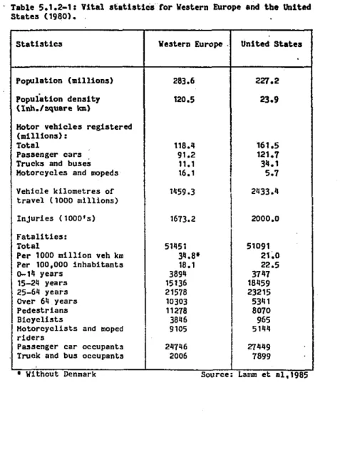
The table below shows the types of data which were collected in a study which attempted to compare road safety between the US and Western Europe.

Hotor v e h i c l e s r e g i s t e r e d ( m i l l i o n s ) :

T o t a l

Passenger cars Trucks and buses notorcycles and mopeds

Table 5.1.2-18 V i t a l s t a t i s t i c s f o r Western Europe and t h e VRitcd

S t a t a s (1980).

I

Vehicle k i l o m e t r e s or

1

1459.3 1 2433.4

t r a v e l (1000 m i l l i o n s )

I

1

I

I n j u r i e s (1000's)

1

1673.2

I

I MOO.0

I

United S t a t e s

227.2 23.9 S t a t i s t i c s

P o p l l a t i o n ( m i l l i o n s ) ~ o p u i s t i o n d e n s i t y ( 1 n h . l q u a r e b)

F a t a l i t i e s : T o t a l

Per 1000 m i l l i o n veh km

Per 100.000 i n h a b i t a n t s 0-14 years

15-24 years 25-64 y e a r s Over 64 years

Pedestrians B i ~ y c l i s t s

Motorcyclists and moped r i d e r s

Passenger car occupants Tru#:k and bus occupants

Western Europe

283.6 120.5

L 1

4.3.

THE SMEED

EQUATION

A further method of comparing fatality rates between countries was put forward by Smeed (1949). He showed empirically by using data from 20 developed countries for the year 1938, that the number of road accident fatalities in these countries was related to the population and the number of motor vehicles, and that this relationship could be described generally by the formula:

where

D

= annual number of fatalities;

N = motor vehicle registrations;

P = population; a,b = constsdts.

By means of a regression analysis, using data from these 20 countries, the constants a and b were shown to be 0.0003 and 213 respectively.

In a later study Smeed examined data for 1930 and 1950 &om 18 of the original 20 countries. Then

in

1970 he examined data from 68 countries for the years 1960-67. In both studies

it

was shown that the above equation still produced good results using the same coefficients. Other authors have also studied the consistency of the Smeed equation. Adams (1985) has shown that the Smeed equation is a reasonably good fit using data from 1980 for 62 countries. A separate study used as near as possible Smeed's original countries and repeated the analysis for the years 1950, 1960 and 1970. The relationships they derived were very similar to those found by Smeed. In 1950 the values of the coefficients were a = 0.00034 and b = 0.58, in 1960 the values were found to be a = 0.00034 and b = 0.60, and finally

in

1970 a = 0.00039 and b = 0.56. In a subsequent analysis of the situation in developing countries, it was shown that in 1968, a = 0.00077 and b = 0.40, and in 1971 a =

0.000914 and

b

= 0.43. It has been suggested that the variation in the value of 'a' is related to the level of safety in a country. Those countries which consistently have values lower than the 0.0003 suggested by Smeed (such as GB) can be said to have higher levels of safety, while countries which have values consistently higher (such as the Federal Republic of Germany) can be said to have lower levels of safety.

It was shown in the original 1949 paper, using data from 1938, that 10 of the 20 derived values of the number of deaths were within 15% of the actual values, 19 were within 4096, and 1 was in error by 67%. Thirty years later, in only 5 out of 70 countries, using 1968 data, is the ratio of the recorded to the predicted number of deaths outside the range 0.5-2.0. 33% of the actual numbers of fatalities are within 15%, and 67 are within 40% of the expected.

Various reasons have been put forward as to why fatality data £ram such differing circumstances should always apparently follow this general pattern. Smeed

himself

says "as the population accident rate becomes higher the urge to do something about

reduction include the trend in technically developed countries for a reduction to occur in the exposure of pedestrians, pedal cyclists, and (until recently) motorcyclists, all of whom have high risk of involvement in road accidents, and of receiving fatal injuries when so involved. For motor vehicles to become safer as technology improves, for the number of kilometres driven per vehicle to decrease as motorisation increases and for a shift to always higher proportions of cars, which are a relatively safe type of vehicle, compared to pedal cycles and motorcycles.

Criticisms of the

Smeed

equation

Most such criticisms seem to concern its accuracy. Numerous studies have found different values of a and b which fit a particular data set better than the original equation. However, Smeed's equation has been found to apply over such a wide range of circumstances, and while it is obviously possible to define a new equation which fits a particular data set more accurately,

it

is unlikely that this new equation will be as widely applicable. The fact that Smeed's equation does not exactly fit all data sets does not detract from its general usefulness. It provides a simple tool in international comparisons, which accounts far the relative size of a country (population) and level of motorisation (number of motor vehicles). It is neither a causal model, giving reasons why this relationship should be so, nor does the equation account for a wide variety of possible influencing factors. It also accommodates within the limits of variation around the basic equation a wide range of values. There is, however, scope for recalibrating Smeed's equation for the post-1973 years in view of the widespread reduction of fatalities experienced since then.

More specific criticisms have been cited in the literature concerning the mathematical techniques used by Smeed and subsequent users of his equation (see Andreassen, 1985). It is questioned whether the original regression equation can be manipulated algebraically to produce some of the derivative forms of the equation. He also considers the inaccuracy of the equation and concludes that Smeed's original analysis of 20 countries for one year of data was just that, and "cannot be extended to predict the number of deaths in any year in any country". This statement is true as it stands, although the Smeed equation can give a very good idea of the likely number of accidents i n a country, but, the real aim of the equation is to identify countries which have large differences between the actual and expected numbers of deaths, and in so doing point towards areas where M e r more detailed research may be rewarding.

The Smeed equation has recently been the subject of considerable debate in mad safety circles. The principle protagonists are probably John Adams from Britain and David Andreassen from Australia. The debate has taken up sizable chunks of the journal TrafTic Engineering and Control recently in terms of articles and letters to the editor. Some of the content of this discussion has been mentioned above, though a much more detailed idea of the arguments should be gained by looking through back issues of the journal Tr&c Engineering and Control for the years 1987 and

1988.

4.4.

OTHER TECHNIQUES

As has already been mentioned, the Smeed equation was a regression equation which considered the effect of two factors upon the number of fatalities caused by motor vehicles (i.e the population and number of motor vehicles). It was shown that a large degree of variation between countries and over a wide variety of time periods can be explained by these two factors.. However, despite this, there is sufficient variation between the actual number of deaths and those predicted by the

equation in many countries, to suggest that other factors also have substantial effects upon the number of accidents. Several studies have attempted to assess how much more accuracy can be gained by using a model with more than 2 factors. These studies use multiple regression techniques.

One particular study carried out in 1975 examined the effect of 6 factors thought to influence mortality rates from motor vehicle accidents. These factors were:

a) the numbers of vehicles per person in the total population; b) the length of roads per unit area of country;

C) the proportion of the population in large urban areas;

d) the proportion of the population under 19 years; e) the proportion of the population over 65 years;

f) the proportion of taxis and private cars in the total number of motor vehicles.

The study used data from 17 european countries for 1970, and concluded that for only three of the variables is there evidence i n these data of a significant relationship with the levels of mortality due to motor vehicle accidents (at the 0.05 level of coniidence). These were factors a, b and e.

Two

other models are worth mentioning briefly here:

1) Sivak's

'Societal

violence, young drivers and accident propensity model': This was a model created by applying multiple regression to 1977 data from each of the individual states in the USA. Traffic fatalities per registered vehicle was the dependent variable. The independent variables were the states' homicide rate, suicide rate, fatality rate from non-tr&c accidents, unemployment rate, personal income, density of physicians, alcohol consumption, motor vehicles per capita, road mileage per vehicle, sex and age distribution of drivers, and attained education. From among these independent variables, only three proved to be significant predictors of traffic fatalities: homicides per capita, proportion of drivers under 25 years of age, and fatality rate from non-traffic accidents. These three variables accounted for 68% of the variance of states' traffic fatality rates. These results suggest the possibility that (a) " society's level of violence and aggression affects the extent of aggressive driving, and, consequently, the frequency of traffic accidents"; and (b) " young drivers are a significant fador in the traffic accident problem, probably because of their lack of experience".

2) Partyka's economic model: This is a model that was based on employment and population data using data from 1960 to 1982. The model was of the following form:

where D = traffic fatalities;

U

= unemployed workers;

E = employed workers;

N = non-labour force (population

-

(U

+

E)).

Model Fatalities Smeed's degree of motorisation model 64,816

Sivak's societal violence model 40,590

Partyka's economic model 54,730

Actual no. of fatalities in 1985 43,795

It can be seen that the Werent models met with differing degrees of success, with

5.

ACCIDENTS, EXPOSURE, RISK AND TRAFFIC FLOWS

5.1. INTRODUCTION

The number of accidents a t a site, along a route or within a n area, during a time period can be considered to depend upon:

(1) the number of potential accident situations that arise (N);

(2) the probability of

an

accident occurring, given a potential accident situation has arisen (p).

The interaction between the exposure N and the

risk

p gives rise to A accidents, where:

Although sites (or routes or areas) may have the same accident exposure during a time period, the number of accidents may differ, because of variations in accident risk, which depends upon local conditions.

The number of accidents can be reduced by:

(1) reducing the exposure N, (2) reducing the risk p.

The accident exposure can be reduced by:

(1) reducing the amount of travel,

(2) traEc management measures (e.g. banning turns across an opposing straight-through movement).

While the accident

risk

can be reduced by trafKc managemenuengineering (e.g. changing intersection layout so that drivers of turning vehicles have a better view of opposing straight-through vehicles and can judge better when the turn can be made safely).

Reducing the amount of travel is outside the scope of this course.

5.2. MODEL ESTIMATION

The number of accidents in a period is observable, but exposure and risk are theoretical concepts and are not observable.

If it is assumed that both risk and exposure are functions of traflic flows alone, then it follows that the number of accidents is also a fhction of traffic flows alone. This assumption is oRen made, despite the fact that it is obviously an

account of thew other fadors (e.g. when devising a new tr&c plan using a traffic management model, such as SATURN).

IE

where:

q = trafiic flow (or flows)

then there are essentially two approaches available for model estimation:

(1) a purely empirical approach, involving finding a relationship directly between the number of accident and traffic flows (risk and exposure are not estimated separately).

(2) a theoretical-empirical approach, involving:

(a) defining N(q) on the basis of theoretical considerations

(b) observing A(q)

(c) obtaining d q ) = A(q)/N(q)

5.3.

LINK

EXPOSURE FUNCTION

The form of the accident exposure function depends upon the type of accident:

(1) single-vehicle accidents (2) rear-end accidents (3) head-on accidents

5.3.1. Single-vehicle accident exposure. " The exposure may be:

(1) time-based (each instant of time a vehicle is on the road amounts to an exposure)

(2) distance-based (each small distance travelled amounts to an exposure)

A vehicle travelling for time T gives rise to (TIAt) exposures, while a vehicle travelling a distance S gives rise to (SlAs) exposures, where:

A t = instant of time As = small distance

In order that the two estimates of exposure are equal, it is necessary that:

where