i
The Estimation of the Rate of Return to
Education in China:
An Empirical Analysis using Instrument Variable
Estimation with Months of Birth and Its Issues.
Michael Leith Cowling
Primary Thesis Advisor: Professor Xin Meng
Research School of Economics
ANU College of Business & Economics
Australian National University
This Sub-Thesis is submitted for the Applied Economic Honours Programme
ii
Abstract
Any attempt to estimate the rate of return to education using ordinary least squares (OLS) models suffers from omitted variable bias due to unobservable factors that are correlated with both the education variable and the return dependent variable. Instrument Variables, such as the birth months of students, provide an alternative estimation method that can create less biased estimates.
The validity of the birth months as instrument variables depends on being uncorrelated with individual personal attributes while having an effect on the education outcome of the individual. However, the exogenous criterion is violated if unobservable factors influences the month of birth and education outcome creating the omitted variable bias problem.
We investigate if the birth month is a good instrument for use in estimating the rate of return to education using empirical evidence from the 2000 Chinese Population Census and the 2009 Chinese Urban Household Income and Expenditure Survey. We split the sample into two groups, individuals with rural education and individuals with urban education due to an urban/rural education gap that the literature captures.
A Two Stage Least Squares Model (TSLS) is run to estimate the rate of return to education and to determine if the instrument birth month variables are strong instruments. We also run an OLS model to compare the OLS rate of return to education with the TSLS estimates. We use the parent’s education level as a proxy for socioeconomic status and investigate if there is a violation of the exclusion restriction for the birth month instruments.
We find students born after August typically achieving a higher education level on average than students born in the August and months before August. In addition, there is a significant and positive rate of return to education using IV estimation which is larger than the OLS estimate of the return to education. We find that parent’s socio economic status either has an insignificant or trivial effect on the timing of births.
iii
Acknowledgements
I would like to express my appreciation and gratitude to everyone who advised and encouraged me throughout the course of the Applied Economics Honours Programme. I am thankful for their guidance and constructive criticism during the Programme and the course of the thesis.
I would like to express my appreciation to Professor Xin Meng for her constructive suggestions and guidance with the background and the empirical work with the thesis. Her willingness to give her time so generously, as my supervisor, has been very much appreciated.
iv
Table of Contents
Page
Introduction 1
Background 6
Data 10
Methodology 12
Results on the Relationship between Birth Months and Education 15 Analysis of the Relationship between Birth Month and Parental Background 17 Rate of Return to Education and Instrument Strength 20
Conclusion 22
Appendix 24
List of Figures 24
List of Tables 45
1
Introduction
According to figures from the International Monetary Fund (IMF), China has overtaken the United States to become the world’s largest economy in 2014. With an economic output a tenth of the US in 1980, the IMF is estimating that China’s economy will soon be 20 per cent larger than the United States (NewsComAu, 2014). China is increasingly playing an important and influential role in the global economy and as a result, we would like to investigate the rate of return to education in China given its history of fast economic growth and its economic position today.
A simple method to estimate the rate of return to education is to use an ordinary least square (OLS) model. However, OLS estimates are biased due to:-
Unobserved ability which biases the returns to schooling upwards1 the observed returns to schooling or downwards2.
Measurement error with the relevant variables which bias the result downwards.
Given the problems faced when using the OLS in estimating the rate to return to education an alternative method proposed in the literature is to use instrumental variable (IV) estimation to identify the causal effect of education on an individual’s earnings.
A classical study by Angrist and Krueger (1991), estimates the effect of education on earnings, using the quarter of the year birth as the instrument. They claim that the quarter of the year birth is an exogenous source of variation in education attainment3 due to the existence of compulsory schooling laws and the fact that most schools in the US begin in September. The month of birth is claimed to be unlikely correlated with the student personal attributes other than their age at school entry.
1
Because high-ability people find it easier to undertake education.
2 Low ability people compensate by completing more education.
3Educational attainment refers to the highest level of education that an individual has completed. This is distinct
2
Angrist and Krueger (1991) find that on average individuals born in the 1st quarter of the year have lower education attainment when compared to individuals born in the 4th quarter due to 1st quarter birth entering school a year later compared to 4th quarter newborns and are more likely to drop out of school before completing a high school degree.
In addition to Angrist and Krueger’s research, there are other studies attempting to establish the relationship between birth months and a student’s education outcome. Bedard and Dhuey (2006) claim that younger students are able to begin accumulating skills taught earlier in school but an older student may be more ready for schooling and hence become more productive.
Datar (2006) states that there are two dominant viewpoints in the childhood literature. The first view is that older children are more mature and that may assist in performing better in school; this is called the ‘absolute age’ effect. The second view is that there is a ‘relative age’ effect which asserts that students born early in a school cohort do better than their peers because of their relative advantage over their peers. This could happen if the curriculum is geared towards the average student’s level of development. Datar found that delaying kindergarten entrance indicates a significant increase in test scores (math and reading).
Elder and Lubotsky (2009) found that having older classmates increases the probability of repeating a grade and being diagnosed with a learning disability, but at the same time increases their achievements in both mathematics and reading.4 They suggested that high performing peers positively influence a student’s achievements but school and parental decisions regarding grade retention and behavior referrals are partly based on a student’s age and performance relative to his classmates.
The past literature has provided ample evidence that there is a birth month effect in which a student’s education outcome is correlated with the time of their birth within the calendar year. Given this relationship and with Angrist and Krueger (1991) and Lam and Miron (1991) claiming that the month of birth is exogenous, it appears that the month of birth dummies can be used as valid instruments for use in the estimation of the rate of return to education in China.
4 These negative peer effects likely arise from the fact that grade progression and the decision to refer a child to a
3
However, recent research has questioned the validity of the birth month dummy variables as instruments on the basis that they may not be exogenous and maybe influenced by unobserved personal factors such as the student’s family background. Buckles and Hungerman (2013) found that there is a strong correlation between the seasonality of births and the seasonality of maternal characteristics. There have been arguments that Angrist and Krueger (1991) estimates were unsatisfactory because of the birth months’ weak correlation with education in certain specifications, mainly those that include age and age square as covariates. (Cruz and Moreira, 2005)
Bound, Jaeger and Backer (1995) and (2001) were unsatisfied with Angrist and Krueger’s results when they find the association between the yearly quarter of birth and education attainment to be weaker in more recently born cohorts. Meanwhile no similar pattern existed in the association between quarter of birth and earnings. They point out that the quarter of birth instruments from Angrist and Krueger (1991) research explains only a trivial proportion of the variation in schooling leading to two distinct problems: - (a) The Two Stage Least Squares (TSLS) estimator with weak instruments is biased in small samples, and (b) any inconsistency from a small violation of the exclusion restriction is magnified by weak instruments.
4
Before there can be any valid inferences of the rate of return to education using the month of birth as instruments for education attainment, the instruments must be uncorrelated with any unobserved factors or variables that may have an influence on the students’ education outcomes. Lam and Miron (1991), which Angrist and Krueger (1991) referenced, claim season of birth is unrelated to the socioeconomic status (SES) of the parents and that seasonal pattern is identical for illegitimate and legitimate births.
Buckles and Hungerman (2013) using data extracted from live birth certificates find that season of birth and later outcomes, including education attainment, are largely driven by the differences in fertility patterns across socioeconomic group. They found large and regular seasonal changes in the socioeconomic characteristics of women giving birth with women giving birth in winter being more likely to be teenagers, less likely to be married or having a high school diploma. Women with higher SES are more likely to give birth in spring rather in winter. There is evidence of family background being strongly related to the timing of newborn, suggesting that the exclusion restriction is not satisfied.
Buckles and Hungerman accept the fact that their seasonality patterns are driven by women wanting a birth but indicated that conditions at the anticipated time of the birth are much more important in accounting for the seasonal patterns observed in their data.
5
However, Bobak and Gjonca (2001) claimed that weather and climate effects in developed countries are weaker because in these countries individual choice is the largest factor and that the differences in birth seasonality between different socioeconomic groups can be due to differences in family planning5. They speculate that it is possible that different socioeconomic groups may have different preferences of the date of birth and concluded that different socio-demographic factors play an important role in shaping seasonal variation in births.
Due to the above concerns regarding the validity of using birth months as IV we will first establish if there is a birth month effect on the level of education achieved before estimating the rate of return to education in China. The data extracted to investigate this issue were the relevant birth month and education data from the 2000 Chinese Population Census and the 2009 Urban Household Income and Expenditure Survey. It was found that there is a birth month effect in both rural and urban samples. We found that students who are relatively older upon school entry achieve on average higher education attainment. We also found the birth month effect to be stronger among urban students when compared to rural students indicating an urban and rural education gap in China.
We also investigate if the birth month instruments are strong instrument variables for use in a TSLS estimation of the rate of return to education. We use the common rule of thumb in which the F-test statistic of the joint test, that the birth month instruments are statistically significant in the first stage regression should be larger than 10. When performing the TSLS estimation using the 2009 Chinese Urban Household Income and Expenditure Survey data we found that the F-test statistic of the joint test to be less than 10 which implies that the birth month instruments are weak.
5
6
Before we conclude on using the birth month dummy variables as valid instrument variables, we investigate the relationship of family background and timing of birth, focusing on birth information on newborns from the census and survey dataset. We investigate if there is a significant relationship between the SES of household heads and the month of birth of newborns. We found that there is similarity in the seasonality of births between high and low socioeconomic parents and that the relationship between the timing of birth and parent background is trivial at most.
Lastly, we ask the question on why family background is not related to the month of birth in China and Taiwan while Buckles and Hungerman (2013) found evidence that the SES of mothers influenced the time of birth.
Background
In China, education is divided into three categories, basic education, higher education and adult education. The ‘Law on Compulsory Education’ was passed in 1986 which states that the Chinese State shall institute a nine-year compulsory education divided into two stages , primary and lower secondary education. The law states that all children, regardless of sex, nationality or race shall attend school when they are age 6 by the 1st of September or postponed to the age of 7 under certain conditions. Compulsory education is provided free of charge. At the stage of non-compulsory education, systems of tuition fees are adopted.
7
Basic education in China includes pre-school education, primary education and regular secondary education. Pre-school can last up to three years, with children entering as early as age three up to age six when they will entry primary education. Enrollment in pre-school education is optional. The academic year typically starts on the 1st of September and they usually have to be age 6 to enter primary education. The year is also divided into two semesters. The length of schooling for primary education is about six or five years and for lower secondary education, four or three years. Children enter lower secondary education at the age of 12 or 13 years.
The starting age for upper secondary schools is 15 or 16 years and the length of schooling is three years. Secondary education is divided into academic secondary or specialized/vocational/technical secondary education. Academic lower and upper middle schools teach academic secondary education. Lower middle school graduates interested in continuing their education can take a local administered exam. The results of the exam will help determine whether the student can choose to enter an academic upper middle school or entering a vocational secondary school.
Vocational schools offer programs ranging from two to four years training as a worker, farmer, managerial or technical personnel. Technical schools typically offer four-year programs to train intermediate technical personnel. For secondary specialized schools, there are two different starting ages. For schools that enroll lower secondary school graduates, the starting age is 15 or 16 with the length of education being three or four years. For schools that enroll upper secondary school graduates and the starting age will be below 22 years. The lengths of these school programs are typically 3 years for upper secondary schools and for upper secondary vocational schools they can last two or three years.
Higher Education at the undergraduate level includes two and three year junior colleges6. Graduate programs are also included leading to either a Master’s or Ph.D. degree. Chinese higher education at the undergraduate level is divided into three and four year programs with the latter being offered at four-year colleges and universities but these programs do not always lead to the bachelor’s degree.
6 They are sometimes called short cycle colleges, four year colleges, and universities offering programs in both
8
Lastly, adult education overlaps all three of the above categories. Adult primary education includes Workers’ Primary Schools, Peasants’ Primary Schools, and literacy classes. Adult secondary education includes specialized secondary schools for cadres, staff and workers, for peasants, in-service teacher training schools and correspondence specialized secondary schools. Adult higher education includes radio/TV universities, cadre institutes, workers’ colleges, peasant colleges, correspondence colleges and education colleges. Most the above offer both two and three year short cycle curricula and only a few offer regular undergraduate curricula.
Since the establishment of the People’s Republic of China (PRC), the Chinese government aimed to build an education policy aimed at promoting economic growth while maintaining an equitable society (Hannum, 1999). Since then, Political priorities regarding education in China changed over the years and exerted an impact on opportunity structures which have differed for rural and urban areas.
Nationwide expansion in education in the early years of the People’s Republic of China aimed at reducing class differences and producing a skilled labor force; under conditions of scarce resources, policy makers chose to capitalize on the faster returns to education building on existing educational infrastructure in urban areas (Hannum, 1999).By 1981, there were 4,016 key point schools7 in China, mostly located in urban areas and enjoying a national funding priority. In contrast responsibility for the administration and financial needs of education in rural areas was delegated to the township and county level.
7
9
Empirical evidence from Hannum found that the number of students, teachers and schools in rural areas declined substantially after growing in the late 1970’s peaking during the Cultural Revolution and dropping drastically after 1978. In rural areas, education (in primary – junior high) progression ratios8 were one rural junior high school entrant for every four primary school graduates while cities and towns had full progression before the Cultural Revolution. After the Revolution, roughly one rural junior high school entrant for every 2 primary school graduates while cities and towns maintained full progression.
Knight and Shi (1996) found that the most important factor influencing a person’s education attainment is whether he lives in a rural or an urban area. The standardized mean difference in education attainment (in years) is no less than 4.6 years in favour of urban students. Furthermore they claim that ethnic and gender discrimination in education is more apparent in rural areas and over half of 14-19 years old rural children had dropped out of based on their analysis of the 1988 national household sample survey.
Given the gap in urban and rural education in China, we will separate our samples into rural and urban education and perform separate analysis to create precise estimates on the return to education? We create a dummy variable indicating if individuals undertook education under rural or urban education based on the individual hukou registration9.
Despite schooling in urban areas are claimed allegedly to be free for migrant students as well, there are still considerable barriers of entry for migrant students and eventually led to the rise of private migrant schools. However they generally have poor teaching, facilities, underdeveloped curriculum and relatively high tuition fees compared to state urban schools (Reap.stanford.edu, n.d.). Therefore we can assume adults with a rural hukou status will have received education this is of less quality than adults with an urban hukou status.
8 Progression Rations was calculated by Hannum to relate the number of entrants to the higher level of education to
graduates of the previous level for the given year.
9 The hukou system is a form of a household registration system which included strict limits on migration and access
10
Data
The data used in this study come from the 2000 Chinese Population Census and from the 2009 Chinese Urban Household Income and Expenditure Survey. China’s National Bureau of Statistics reported that mainland China population totaled 1.266 billion individuals with urban population totaling 455.94 million individuals or 36.01% of the population.
Before we analyze the effect of birth month on education attainment and the relationship (if any) between parental background characteristics and the time of birth, we may have to first separate our data into individuals who undertook rural and urban education due to differences in quality of education and socioeconomic characteristics for rural and urban individuals following the education gap we have discussed in the section above. Overall we have 5,065,293 observations for our rural sample and 1,888,586 observations for urban sample from the 2000 Chinese Population Census data. We will also be using the 2009 Chinese Urban Household Income and Expenditure Survey to investigate the birth month effect on education attainment.
The urban survey focuses mainly on collecting household expenditures and incomes but also contains sections covering household characteristics (Gibson, Huang and Rozelle, 2003). The survey collected data through a combination of diary keeping and questionnaire interviews and requires respondents to keep a daily expenditure diary for a full 12 month period and stay in the program for 3 years. From the urban survey data, we will focus our analysis on individuals with an urban hukou status for which we have 80,202 observations.
11
Yet, Chinese census data lacks the income information necessary in order for us to run TSLS estimation with the education variable being instrumented by the month of births. Instead we will make use of the 2009 Chinese Urban Household Income and Expenditure Survey data to perform such estimation. In addition, we would also like to perform the TSLS estimation with individuals aged between 22 and 65 years as they would also likely have some form of employment or income. We have 74,634 observations to analyze from individuals with urban hukou status.
To investigate if there is a relationship with the individual birth month and the household head SES, we will make use of samples containing individuals whose ages are less than 22 years. This choice is because of selection issues. If we included individuals above 22 years old as the older the individual, the less likely he/she resides with their parents in the same household. We may face selection issues in our sample if we include households that have an ‘adult’10
child as they would have made a deliberate decision to continue living with their parents due to social and/or economic factors that are currently unobservable to the research. We limit our observations on ‘children’ that are aged 22 years and younger to limit self-selection bias on the assumption that they’d be too ‘young’ to determine to move out of the households.
For our analysis regarding the relationship between parental background and time of birth we will be using the head of the household as proxy for parents and identify individuals who reported as the ‘child’ to the household head. We will ignore any other observations that are not described as the head or the child of the household and for each household ID, there has to be at least one parent and one child. As a result our sample will have 1,011,287 observations for the rural sample and 192,856 observations for the urban sample from the 2000 Chinese Population Census data.
10 An observation is an adult child if he/she is aged more than 22 years of age and is identified as a child in a
12
From the urban survey, we have 18,792 observations to analyze and our analysis will be focused on individuals with the urban hukou status. Summary statistics are available from Table 1A (page 45) for the 2000 Chinese Census data and Table 1B (page 47) for the 2009 Urban Household Income and Expenditure Survey data in the appendix but we can see that our concerns regarding the education gap is well justified especially seeing that the mean level of education attainment for urban individuals are higher than the rural individuals.
Methodology
To estimate the rate of return to education, we will use a Two Stage Least Squares Model using the birth months as our instrument variables. The first stage equation will involve a regression of the education outcome against the birth month dummies. The literature investigates the birth month impact on education outcomes using different dependent variables such as test scores and education attainment. Given our data set and our goal, the endogenous education variable that we have available for use is the level of education achieved.
Additional controls are used in the literature to take into account of the individual’s personal observable characteristics such as marital status, gender and location of residence. Since we have this information in our data sets we will use it in our TSLS models. We then run the TSLS model below using the 2009 urban survey data mostly focusing on individuals registered with an urban hukou status.
∑ ∑ ∑ – (1)
∑ ∑ – (2)
represents the highest level of education attained by individual i.
is the natural log of individual i’s annual income
represents a dummy variable indicating if individual i was born in month c.
13
is a dummy variable that indicates if the ith individual is residing in
province d in China. The omitted categorical province variable will be Beijing for both the census and urban survey data.
is a dummy variable controlling for the year of birth for individual i.
Equation (1) will be the first stage regression and equation (2) will be the second stage regression. The second stage equation includes the coefficient will represent the percentage change in individual i’s income for attaining an additional level of education.11
The basic purpose of TSLS estimation is to avoid the bias that OLS model suffers due to omitted variable bias and measurement error. However, it has been established that TSLS will estimate with a bias in all finite sample sizes (Murray, 2006). The TSLS estimator is at most biased when the instruments are weak and if the instruments are many, the estimator can be biased toward the probability limit of the OLS estimate of the return to education. Stock, Wright and Yogo (2002) suggests a rule of thumb in which the F-statistic of a joint test, whether all excluded instruments (The birth month instruments in this case) are significant, should be above 10. This will indicate that we do not have a weak instrument problem. Murray (2006) suggests another rough rule of thumb, when the size of the sample used times the of the first stage of the TSLS model is larger than the number of instruments, the TSLS estimates tend to be less biased than OLS estimates. Our analysis will include applying these two ‘rules’ to our results.
We will investigate if there is a correlation between the month of birth and the level of education achieved using both the 2000 Chinese Population Census data and the 2009 Chinese Urban Household Income and Expenditure Survey and running regression (1) with both data sets. For the urban survey, considering that individuals with a rural hukou status are in the minority in this sample, we perform the analysis by focusing mostly on individuals with an urban hukou status.
11
14
If there is a relationship between timing of birth and the education attainment, than the coefficient estimates should be statistically significantly different from zero. In addition we investigate if the pattern of the coefficients is in line with the past literature. We will run the regression separately for rural and urban samples. The omitted categorical birth month variable will be August as August Born children attend a school around a year earlier compared to September born children and they will be the youngest in their class.
We will compare the education attainment achieved by the students born before and after August and we will confirm if there is a similar pattern or trend that the past literature has established i.e., if earlier or later born entrants have an advantage in terms of the education level attained. The coefficient is the additional education an individual i, born in month c, will attain when compared to an individual born in August. Furthermore, we will also test for the strength of the instrument in the TSLS model and investigate if the rate of return for education estimates is less biased than their OLS counterparts.
Buckles and Hungerman (2013) raised concerns that the time of birth is not exogenous. As a result, the next step in our analysis is to attempt to see if there is any relation between the timing of birth and the observation’s parents’ SES and if the exclusion restriction holds. To investigate this relationship, we use the household head (mother or father) education attainment as an indicator of low and high SES. We assume household heads that completed secondary school education or above are of high SES while household heads who did not complete it, will be of low SES.
15
∑ ∑ ∑ – (3)
where is a dummy variable that indicates if individual i has a parent that completed secondary school education.
We will separate our analysis for rural and urban samples. To conclude that there is no relationship between household heads education and the observation’s birth month it would require the birth month dummies to be statistically insignificant or for its coefficients to represent only a minimal effect.
Results on the Relationship between Birth Months and Education
We first run equation (1) using the census data separately for rural and urban individuals. The results we generated will appear starting in the appendix section of this research. The results for equation (1) are listed in Table 2A12 (page 49) for the rural sample and in Table 2B (page 50) for the urban sample. In Table 2A, we found February to be statistically insignificant while in Table 2B, the birth months March, April and July are statistically insignificant. We estimate equation (1) again using data from the 2009 Chinese Urban Household Income and Expenditure Survey and we place the relevant results in Table 3 (page 51). The table shows that the birth months July, September, October, November and December are statistically significant while the other months are statistically insignificant. Overall there does appear to be a relationship between the month of birth and the level of education attained.
12 For Tables 2A to Table 6C, we report only the birth month coefficients and for Table 6A and 6B, we report only
16
Table 2A, Table 2B and Table 3 shows that students born after August in September, October, November and December achieve, on average, a slightly higher education level compared to students born in the other months.13 From the background section we understand that in China, September is generally the month of school entry for students when they have reached the eligible age. In a given year, eligible students born in the months before September generally enter school together with eligible students born in September (students that are born after the beginning of September), October, November and December from an earlier birth year cohort14.
The ‘latter born’15
students are relatively older and hence more ‘mature’ than their classmates who were born in the months before September. From both Tables 2A, 2B and Table 3, the results from the urban and rural samples seem to suggest that students who are relatively more mature on school entry achieve, on average, a higher education level than their younger classmates.
We acknowledge that the coefficient estimates for the September birth month in Tables 2A, 2B and 3 might be sensitive due to the fact that students born in September can gain early entry into school. For example, the school administration can be lenient to certain September born students who were born only a few days after the 1st of September. They can be given permission enter school earlier than the other students born late in September whom have to wait another year before they reach the eligible age required for school entry.
In addition, we find that the coefficients appear to have a higher impact on education attainment for urban individuals when we compare them to the rural individuals. We illustrate the birth month coefficients in Figure 3 (page 36) and we can see that the urban individuals have a stronger positive education effect compared to the rural sample from July to January (Omitting the August birth month) and a stronger negative effect from February to June, highlighting the rural and urban education gap we discussed in the background section above.
13
There is an exception in Table 3, where January born students achieve an education level that is higher than students born after August. However, the coefficient estimate for January is statistically insignificant in Table 3.
14 For example, students born before September in 1990 are expected to enter school together with students born in
September, October, November and December in the year 1989.
17
We infer from our results that there does appear to be a birth month effect on education attainment. There appears to be a maturity and an ‘absolute age’ effect occurring within our sample where the older students in a classroom are able to achieve a higher education level than their younger classmates. This appears to be in line with the conclusions reached by the past literature such as Bedard and Dhuey (2006) and Datar (2006) where ‘older’ children at school entry are more prepared for schooling creating a positive effect on education attainment.
On the other hand, our results also appear to go against Angrist and Krueger (1991) conclusions where relatively younger classmates achieve on average higher education attainment. This could be due to the fact that compulsory education laws in China were only implemented in 1986 when compared to the implementation of compulsory education laws in the United States where by 1930, all of the states in the US had some form of compulsory education implemented (Gelbrich, 1999). This means that a sizeable portion of our sample may not have been subjected to the enforcement mechanisms of compulsory education laws as described by Angrist and Krueger.
Analysis of the Relationship between Birth Month and Parental Background
Buckles and Hungerman (2013) find that children born in January are likely to be born to women who lack a high school education and other factors indicating of being of low SES. This could be due to that high SES mothers are avoiding having their births in winter months. Buckles and Hungerman found a seasonality pattern in the time of birth with the number of births peaking in September and the trough located in December or January. On the other hand, Fan Liu and Chen (2014) found that in Taiwan, the number of births peak in October while April had the lowest number of births in a year making the seasonality pattern of births different between the two countries.
18
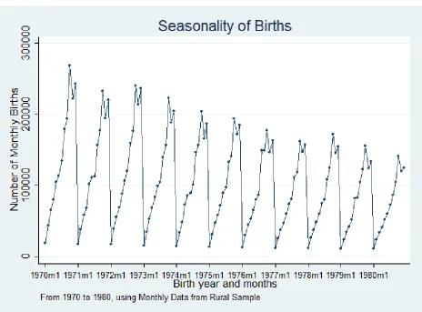
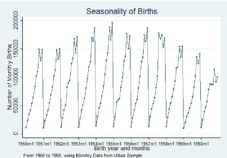
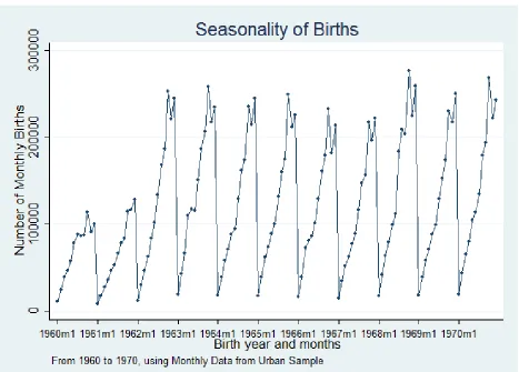
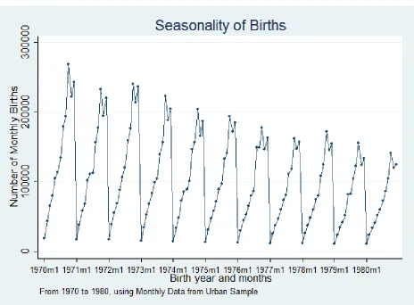
In both the rural and urban samples, we can see that like many other countries, the number of births over the years displays a persistent pattern of seasonality. The seasonality pattern is different when compared with Fan, Liu and Chen’s results but are almost surprisingly similar with Buckles and Hungerman results. January appears to have the lowest number of new births per year while the number of newborns appears to be consistently peaking in October.
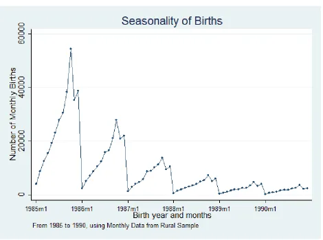
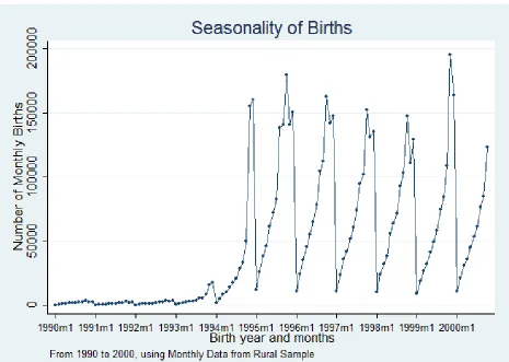
An interesting feature seen in Figures 1E, 1F, 2E and 2F is the drastic fall in the number of newborns just before 1990 and the subsequent rapid rise only after 1994. This pattern may have been caused by the enforcement of the one child policy16.
While Buckles and Hungerman find that there is a correlation between the month of birth and the SES of mothers, Fan, Liu and Chen found the seasonality pattern of birth to be strongly similar between high and low SES mothers. Fan, Liu and Chen speculate on the reason for this difference in relationship between parental background factors and month of birth. In order to add to this speculation, we attempt to investigate the seasonality pattern of births between high and low SES household heads in China using secondary school completion as an indicator of social economic status.
In order to determine if there is a seasonality pattern between the month of birth of the individuals in China and the SES of their household head, a simple method would be to directly examine whether births to household heads with different SES levels exhibit different patterns of seasonality. We compare monthly newborns to household heads completing secondary education (also known as high SES household heads) with newborns to household heads with lower education levels (which represents low SES household heads).
We graph the births of individuals aged less than 22 years and the results can be viewed in Figure 4A to Figure 4D for the rural sample and Figure 5A to Figure 5D for the urban sample. We perform a similar analysis using the urban survey data and the seasonality pattern can be viewed in Figure 6A to 6B. These figures appear in pages 37 to 44.
16 The policy was implemented in 1979 and consists of a set of regulations governing the size of Chinese Families.
19
In all of Figures 4, 5 and 6 we see that the curves do not exhibit any clear pattern of seasonality which implies that SES of household heads may not determine the month of birth. To test the non-correlation between month of birth and parental SES formally we ran the linear equation (3) separately for the rural and urban samples using the 2000 Chinese Population Census data and individuals aged less than 22 years of age.
In our analysis we set the August birth month as our omitted categorical variable. Looking at Table 4A (page 52), the birth month dummies for the rural sample appear to be statistically insignificant. From this we can conclude that does not appear to be any relation between the birth months and the SES of household heads for rural individuals.
Table 4B (page 53) contains the regression output from running equation (3) using only the urban sample. We see that most of the birth month dummies have coefficients statistically insignificant at 1% significance except for the September dummy. Despite this, the coefficient for the September birth month dummy indicates only a minimal increase in the probability of having a household head with secondary school education or higher. We can conclude there is no conclusive evidence of a seasonality relationship with the SES of the household head and the time of birth.
Using the urban survey data, we look at individuals with an urban hukou status and less than 22 years of age. With the given criteria, we have 18,792 observations for analysis and found that at 1% significance, the birth month dummies coefficients are statistically insignificant. The relevant results are placed in Table 5 (page 54) and they tell us that there is no relationship between birth month and the socioeconomic characteristic of the household head. Our results and conclusions coincide with Fan, Liu and Chen’s paper in that month of birth is found to be exogenous and is unrelated to the household head education background.
20
Buckles and Hungerman argue that, in the United States, expected weather conditions are an important factor in creating the different seasonality birth patterns between high and low SES women. Since the weather varies across China with cities such as Shanghai experiencing mild winters and moderate weather in the Southeast Provinces while regions such as Beijing experiencing dry, cold and long winters along with snowy winters in the Northeast provinces, we would expect that China would be a factor influencing different seasonality birth patterns.
Given that regions in China vary its weather conditions due to its geography, it is important that we control for the residential location of the individuals in our sample. Despite experiencing both harsh and mild winters, China experiences the same non-seasonality pattern between high and low SES parents such as Taiwan. We can speculate that weather may not be a good explanation for this occurrence but Bobak and Gjonca (2001) provide another possible explanation, which is different socio-demographic factors could play an important role in shaping the seasonal pattern in births especially among high and low SES mothers.
Buckles and Hungerman (2013) results are clearly at odds with the result we have found where they show that there are significant differences in the seasonal pattern of births between high and low SES women. Given the trivial difference we have found between the seasonal patterns between high and low SES household heads in our data, we conclude that the month of birth is not influenced by the education levels of the household head and hence the exclusion restriction holds for the birth month instruments.
Rate of Return to Education and Instrument Strength
21
We store the estimates we generate using the OLS model in Table 6A (page 55) and we see that the OLS rate of return to education is statistically significant. This implies that an additional level of education will increase annual earnings by 21.3%. However, we learn that the OLS estimate of the return to education tends to be biased due to omitted variable bias.
To analyze the extent of the bias, we run the TSLS model described in the methodology section and estimate the rate of return to education. The relevant results can be found in Table 6B (page 56) for individuals aged 22 to 65. We see that for an additional level of education achieved, the individual increases their total annual income by 28.8% and that the education variable coefficient is statistically significant. The results suggest that our OLS results suffers from downward bias given the greater returns estimated under the TSLS model. In addition, we find the differences (downward bias) between the OLS and the TSLS estimates to be around 7.5 percentage points.
We then test the strength of our instruments used in the TSLS model by running a joint test whether all of the birth month instruments are significant. We report the robust F-test statistic in Table 6C (page 56) and see that the robust F-test statistic is 5.16. Given that the F-test statistic is below 10, this suggests that our instruments are weak.
22
Conclusion
We have found that, using the 2000 Chinese Population Census and 2009 Chinese Urban Household Income and Expenditure Survey data, students born after August attain, on average, higher education compared to students born before and on August. Based on our understanding of the Chinese School System, students born after August will enter school at a higher age when compared to students born in the other months implying a positive maturity effect on education attainment.
We also examine if there is a relationship between month of birth and omitted variables that can create a link between education attainment and month of birth. In our analysis, we discover that the relationship between parental education and birth month of newborns are non-existent or at the very most trivial, leading us to conclude that the birth month instruments satisfy the exclusion restriction.
Given these findings, there is speculation if geographic and weather factors can explain the different seasonality patterns of high and low SES parents in the USA, Taiwan and China. China has varying weather conditions with harsh winters in the North and milder ones in the South of China. There is still the question of why there is a relationship between parental background characteristics in the United States but not in Taiwan and China. We speculate that it could be due to difference in the socio-demographic of the population according to Boback and Gjorca (2001). We suggest that future research should look for more solid evidence if this is the case and any other underlying reason for the relationship between family background variables and the month of birth of newborns.
23
However, we discovered that our instruments fail to satisfy the F-test statistic rule of thumb, implying that the birth month instruments are weak. We use a rough rule of thumb that suggested that our TSLS rate of return to education estimate is less biased than the OLS rate of return to education estimate. Future research should investigate for a stronger instrument for use to estimate the rate of return to education in China.
What are the policy implications of our results and are the differences in education and income due to month of birth significant enough to warrant a policy response and if so what type of a policy response will be needed? Crawford, Daerdan and Meghir (2007) state that the disparities in education attainment, due to month of birth, remain significant at ages 16 and 18 and they affect decisions related pursuing higher education or entering the labour market. They claim this was not optimal from an efficiency and equity perspective and some form of policy change is needed to limit the inequity. We consider a few policy solutions that governments and schools can consider in order to minimize the month of birth effect:-
Lang and Barua (2012) suggested having a waiver policy which gives students the choice to enter earlier than the legally established age that could increase education attainment especially among groups with a high dropout rate.
We can also consider moving the school entry date earlier or later in the year Bedard and Dhuey (2012) describe this policy to be popular due to the short term cost savings and the thought that it can improve inter-state test score comparisons in the US.
24
Appendix
Figure 1A
Seasonality of Births from 1950 to 1960 of Rural Individuals
25
Figure 1B
Seasonality of Births from 1960 to 1970 of Rural Individuals
26
Figure 1C
Seasonality of Births from 1970 to 1980 of Rural Individuals
27
Figure 1D
Seasonality of Births from 1980 to 1985 of Rural Individuals
28
Figure 1E
Seasonality of Births from 1985 to 1990 of Rural Individuals
29
Figure 1F
Seasonality of Births from 1990 to 2000 of Rural Individuals
30
Figure 2A
Seasonality of Births from 1950 to 1960 of Urban Individuals
31
Figure 2B
Seasonality of Births from 1960 to 1970 of Urban Individuals
32
Figure 2C
Seasonality of Births from 1970 to 1980 of Urban Individuals
33
Figure 2D
Seasonality of Births from 1980 to 1985 of Urban Individuals
34
Figure 2E
Seasonality of Births from 1985 to 1990 of Urban Individuals
35
Figure 2F
Seasonality of Births from 1990 to 2000 of Urban Individuals
36
Figure 3
37
Figure 4A
Percentage of Parents that Completed Secondary School from 1978 to 1985 from Rural Individuals
38
Figure 4B
Percentage of Parents that Completed Secondary School from 1985 to 1995 from Rural Individuals
39
Figure 4C
Percentage of Parents that Completed Secondary School from 1995 to 2000 from Rural Individuals
40
Figure 5A
Percentage of Parents that Completed Secondary School from 1978 to 1985 from Urban Individuals
41
Figure 5B
Percentage of Parents that Completed Secondary School from 1985 to 1995 from Urban Individuals
42
Figure 5C
Percentage of Parents that Completed Secondary School from 1995 to 2000 from Urban Individuals
43
Figure 6A
Percentage of Parents that Completed Secondary School from 1988 to 1998 from Urban Individuals
44
Figure 6B
Percentage of Parents that Completed Secondary School from 1998 to 2008 from Urban Individuals
45
Table 1A
Summary Statistics of 2000 Chinese Population Census Data
Rural Mean
Standard
Deviation Urban Mean
Standard Deviation
Education
(“Everyone between the ages of 22 and 65 years”)
Literacy Class 0.0255476 0.1577812 0.004606 0.067712
Primary 0.41671 0.493014 0.114178 0.318027
Junior High 0.4114907 0.4921038 0.353906 0.47818
High School 0.0551915 0.2283536 0.214511 0.410483
Secondary 0.0055562 0.0743328 0.119738 0.324655
University Specialist 0.0018244 0.0426737 0.120637 0.325705
University Undergraduate 0.0001504 0.0122643 0.050593 0.219166
Graduate Student 0.0000134 0.0036639 0.003117 0.05574
Parental Education
(“With children less than the age of 22 years”)
No Schooling 0 0 0 0
Literacy Class 0.0143605 0.118972 0.00207 0.045445
Primary 0.3919454 0.4881849 0.090351 0.286684
Junior High 0.4771059 0.4994759 0.373803 0.483814
High School 0.0715478 0.2577378 0.211626 0.408463
Secondary 0.0044502 0.066561 0.117052 0.321483
University Specialist 0.0014393 0.0379108 0.137343 0.34421
46
Rural Mean
Standard
Deviation Urban Mean
Standard Deviation
Graduate Student 0.0000156 0.0039536 0.003873 0.062113
Children' Education
(“Less than the age of 22 years”)
No Schooling 0.0789867 0.2697182 0.06323 0.243378
Literacy Class 0.0024589 0.049526 0.000115 0.01074
Primary 0.2537731 0.4351696 0.05046 0.218893
Junior High 0.6088543 0.4880073 0.377214 0.484692
High School 0.0357151 0.1855792 0.191802 0.393721
Secondary 0.0149039 0.1211683 0.254248 0.43544
University Specialist 0.0009178 0.0302812 0.046191 0.2099
0.060458 University Undergraduate 0.0000582 0.0076299 0.003669
Graduate Student 8.56E-06 0.002926 1.15E-05 0.003397
Education Attainment 3.354093 0.9746414 4.854324 1.495918
Observations
("Everyone between the ages of 22
and 65 years") 5,065,293 1,888,586
Observations
("Children Individuals under the
age of 22 years”) 1,011,287 192,856
Observations
("Household Heads with under the
47
Table 1B
Summary Statistics for 2009 Urban Survey Data
Urban Mean
Standard Deviation
Education
(“Everyone between the agse of 22 and 65 years”)
Illiterate 0.0015461 0.0392903
3 year primary 0.0480287 0.2138283
Primary 0.2639086 0.4407531
Junior high 0.2336101 0.4231296
Senior high 0.1028403 0.3037521
Technical school 0.1999202 0.3999426
3-year college 0.1334505 0.3400631
University 0.0114461 0.1063731
Parental Education
(“With children less than the age of 22 years”)
Illiterate 0.0043636 0.065914
3 year primary 0.0000532 0.007294
Primary 0.3421137 0.474430
Junior high 0.1941784 0.395577
Senior high 0.1978501 0.398389
Technical school 0.0264474 0.160466
3-year college 0.0371435 0.189118
48
Urban Mean
Standard Deviation
Children' Education
(“Less than the age of 22 years”)
Illiterate 0.0003411 0.0184669
3 year primary 0.020581 0.141981
Primary 0.2137131 0.4099383
Junior high 0.239013 0.4264928
Senior high 0.0966513 0.2954908
Technical school 0.2352607 0.4241737
3-year college 0.176076 0.3808956
University 0.0169993 0.1292719
Education Attainment 5.563215 1.58854
Observations
("Everyone between the ages of 22 and 65 years")
80,202
Observations
("Children Individuals under the age of 22 years”)
18,792
Observations
("Household Heads with under the age of 22 years Children")
49
Table 2A
Effect of Birth Month on Education Attainment of Rural Individuals Linear regression, absorbing birth year indicators
Number of Observations = 5,065,293 F( 42,2479891) = 16164.57
Prob > F = 0
R-squared = 0.2855
Adj R-squared = 0.2855
Root MSE = 0.8238
Education
Attainment Coefficient Std. Err. t P>t [95% Conf. Interval]
Constant 3.923437** 0.005275 743.77 0 3.913098 3.933776
Birth Month Dummies
January 0.0060006** 0.0018212 3.29 0.001 0.0024311 0.00957
February 0.0019396 0.0017578 1.1 0.27 -0.0015055 0.005385
March -0.0085011** 0.0017633 -4.82 0 -0.0119571 -0.00505
April -0.0120741** 0.0017883 -6.75 0 -0.0155792 -0.00857
May -0.0138959** 0.0017944 -7.74 0 -0.0174129 -0.01038
June -0.0101476** 0.0018002 -5.64 0 -0.013676 -0.00662
July -0.0072872** 0.0017698 -4.12 0 -0.0107559 -0.00382
September 0.0189058** 0.0017365 10.89 0 0.0155023 0.022309
October 0.0231161** 0.0016738 13.81 0 0.0198355 0.026397
November 0.0379428** 0.0017706 21.43 0 0.0344724 0.041413
December 0.0343261** 0.0017546 19.56 0 0.0308872 0.037765
Note: Standard error adjusted for 2,479,892 clusters at the family/household level. Observations are aged between 22 and 65 years and come from the 2000 Chinese Population Census. We control for gender, province residence and birth year but omit reporting their coefficients.
50
Table 2B
Effect of Birth Month on Education Attainment of Urban Individuals Linear regression, absorbing birth year indicators
Number of Observations = 1,888,586 F( 42,1017503) = 1929.16
Prob > F = 0
R-squared = 0.1258
Adj R-squared = 0.1257
Root MSE = 1.3987
Education
Attainment Coefficient Std. Err. t P>t [95% Conf. Interval]
Constant 5.744858** 0.0096392 595.99 0 5.725966 5.763751
Birth Month Dummies
January 0.0204045** 0.0050596 4.03 0 0.0104879 0.030321
February -0.0305598** 0.0049385 -6.19 0 -0.0402391 -0.02088
March -0.0083834 0.0049552 -1.69 0.091 -0.0180955 0.001329
April -0.0075129 0.0050815 -1.48 0.139 -0.0174725 0.002447
May -0.0216388** 0.0050142 -4.32 0 -0.0314664 -0.01181
June -0.0275031** 0.0050361 -5.46 0 -0.0373737 -0.01763
July 0.0017837 0.0049738 0.36 0.72 -0.0079648 0.011532
September 0.0511275** 0.004874 10.49 0 0.0415747 0.06068
October 0.0825368** 0.0046328 17.82 0 0.0734566 0.091617
November 0.1015134** 0.0049111 20.67 0 0.0918879 0.111139
December 0.0930722** 0.0048686 19.12 0 0.0835298 0.102615
Note: Standard error adjusted for 1,017,504 clusters at the family/household level. Observations are aged between 22 and 65 years and extracted from the 2000 Chinese Population Census. We control for gender, province residence and birth year but omit reporting their coefficients.
51
Table 3
Effect of Birth Month on Education Attainment of Urban Individuals Linear regression, absorbing birth year indicators
Number of Observations = 80,202 F( 42,1017503) = 1929.16
Prob > F = 0
R-squared = 0.1258
Adj R-squared = 0.1257
Root MSE = 1.3987
Education
Attainment Coefficient Std. Err. t P>t [95% Conf. Interval]
Constant 6.610627** 0.0267759 246.89 0 6.558145 6.663108
Birth Month Dummies
January 0.0098902 0.024237 0.41 0.683 -0.037615 0.057395
February 0.0042247 0.024279 0.17 0.862 -0.0433629 0.051812
March 0.019302 0.0243664 0.79 0.428 -0.0284567 0.067061
April -0.017713 0.0251484 -0.7 0.481 -0.0670046 0.031579
May -0.0398637 0.0246573 -1.62 0.106 -0.0881928 0.008465
June -0.0110356 0.0245561 -0.45 0.653 -0.0591663 0.037095
July 0.0498513* 0.0249171 2 0.045 0.001013 0.09869
September 0.0606273* 0.0246294 2.46 0.014 0.012353 0.108902
October 0.0542273* 0.0229989 2.36 0.018 0.0091487 0.099306
November 0.0830248** 0.0243113 3.42 0.001 0.035374 0.130676
December 0.0976287** 0.0240542 4.06 0 0.0504818 0.144776
52
Table 4A
Seasonality of Household Head Education using Rural Individuals Linear Regression, absorbing Birth Year Indicators
Number of Observations = 1,011,287 F( 42,1011223) = 35.58
Prob > F = 0
R-squared = 0.0021
Adj R-squared = 0.002
Root MSE = 0.1279
Parent Education
Status Coefficient Std. Err. t P>t [95% Conf. Interval]
Constant 0.0158034** 0.0023671 6.68 0 0.011164 0.020443
Birth Month Dummies
January -0.000018 0.0004666 -0.04 0.969 -0.0009325 0.000897
February -0.0002444 0.0004545 -0.54 0.591 -0.0011352 0.000647
March 0.0000968 0.0004612 0.21 0.834 -0.0008072 0.001001
April -0.0003579 0.000461 -0.78 0.438 -0.0012615 0.000546
May -0.0005818 0.0004642 -1.25 0.21 -0.0014916 0.000328
June -0.0004272 0.0004629 -0.92 0.356 -0.0013344 0.00048
July 0.0002107 0.0004696 0.45 0.654 -0.0007097 0.001131
September -0.0000332 0.0004449 -0.07 0.941 -0.0009052 0.000839
October 0.0002632 0.0004282 0.61 0.539 -0.000576 0.001103
November 0.0002175 0.000457 0.48 0.634 -0.0006782 0.001113
December 0.0006224 0.000467 1.33 0.183 -0.0002929 0.001538
Note: Standard error adjusted for 815,723 clusters at the family/household level. Observations are aged between less than 22 years and extracted from the 2000 Chinese Population Census data. We control for gender, province residence and birth year but omit reporting their coefficients.
53
Table 4B
Seasonality of Household Head Education using Urban Individuals Linear Regression, absorbing Birth Year Indicators
Number of Observations = 192,856 F( 42,1011223) = 57.81
Prob > F = 0
R-squared = 0.1041
Adj R-squared = 0.1038
Root MSE = 0.4279
Parent Education
Status Coefficient Std. Err. t P>t [95% Conf. Interval]
Constant 0.4300837** 0.0089991 47.79 0 0.4124456 0.447722
Birth Month Dummies
January -0.0003924 0.0047492 -0.08 0.934 -0.0097007 0.008916
February -0.0108781* 0.0047154 -2.31 0.021 -0.0201201 -0.00164
March -0.0104303* 0.0047484 -2.2 0.028 -0.0197372 -0.00112
April 0.0020952 0.0048853 0.43 0.668 -0.0074798 0.01167
May 0.002091 0.0048456 0.43 0.666 -0.0074063 0.011588
June -0.0040006 0.0048242 -0.83 0.407 -0.0134559 0.005455
July -0.0024242 0.0048065 -0.5 0.614 -0.0118448 0.006996
September -0.0136928** 0.0047305 -2.89 0.004 -0.0229644 -0.00442
October -0.0045956 0.0045488 -1.01 0.312 -0.0135111 0.00432
November 0.0059421 0.004758 1.25 0.212 -0.0033836 0.015268
December 0.0011037 0.0048493 0.23 0.82 -0.0084009 0.010608
Note: Standard error adjusted for 183,213 clusters at the family/household level. Observations are aged between less than 22 years and extracted from the 2000 Chinese Population Census. We control for gender, province residence and birth year but omit reporting their coefficients.
54
Table 5
Seasonality of Household Head Education using Urban Individuals Linear Regression, absorbing Birth Year Indicators
Number of Observations = 18,792 F( 42,1011223) = 18.2
Prob > F = 0
R-squared = 0.0843
Adj R-squared = 0.082
Root MSE = 0.479
Parent Education
Status Coefficient Std. Err. t P>t [95% Conf. Interval]
Constant 0.6225939 0.0192355 32.37 0 0.5848904 0.660297
Birth Month Dummies
January 0.0175107 0.0169164 1.04 0.301 -0.0156472 0.050669
February 0.0339259* 0.0172431 1.97 0.049 0.0001278 0.067724
March 0.0106846 0.0166371 0.64 0.521 -0.0219259 0.043295
April 0.0192123 0.0172661 1.11 0.266 -0.0146309 0.053056
May 0.0057157 0.0167757 0.34 0.733 -0.0271664 0.038598
June 0.0106735 0.0170192 0.63 0.531 -0.0226858 0.044033
July 0.0149642 0.016998 0.88 0.379 -0.0183535 0.048282
September 0.0390678* 0.0173245 2.26 0.024 0.00511 0.073026
October 0.0312271 0.0165222 1.89 0.059 -0.0011581 0.063612
November 0.0023656 0.0172429 0.14 0.891 -0.0314322 0.036163
December 0.0118017 0.0175732 0.67 0.502 -0.0226434 0.046247
Note: Standard error adjusted for 17,621 clusters at the family/household level. Observations are aged between less than 22 years and extracted from the 2009 China Urban Household Income and Expenditure Survey. We control for gender, province residence and birth year but omit reporting their coefficients.
55
Table 6A
Ordinary Least Squares Estimate of the Rate of Return using Urban Individuals Linear Regression, absorbing Birth Year Indicators
Number of Observations = 74,634 Wald chi2(17) = 1193.43
Prob > F = 0
R-squared = 0.2540
Adj. R-squared = 0.2534
Root MSE = 0.7718
Ln(Income) Coefficient Std. Err. z P>z [95% Conf. Interval]
Constant 9.498418** 0.0171112 555.10 0.000 9.46499 9.531956 Education
Attainment
0.2131948** 0.0021361 99.80 0.000 0.209008 0.2173817
Note: Observations are aged between 22 and 65 years and extracted from the 2009 China Urban Household Income and Expenditure Survey. Standard Error adjusted for 36,755 clusters in total. We control for gender, province residence and birth year in the 1st stage and 2nd stage equations but omit reporting their coefficients.
56
Table 6B
Two Stage Least Squares Estimate of the Rate of Return using Urban Individuals Instrumental Variables (2SLS) IV Regression
Number of Observations = 74,634 Wald chi2(17) = 13537.49
Prob > chi2 = 0
R-squared = 0.2400
Root MSE = 0.7786
Ln(Income) Coefficient Std. Err. z P>z [95% Conf. Interval]
Constant 7.84027** 0.5322351 14.73 0.000 6.797108 8.883431 Education
Attainment
0.2876108** 0.0721069 3.99 0.000 0.1462838 0.4289378
Note: Observations are aged between 22 and 65 years and extracted from the 2009 China Urban Household Income and Expenditure Survey. Standard Error adjusted for 36,755 clusters in total. Instruments used are the province dummies, male dummy, birth month dummies and the birth year dummies. We control for gender, province residence and birth year in the 1st stage equation but omit reporting their coefficients.
*p<.05, **p<.01
Table 6C
Test of strength of birth month instruments First-stage regression summary statistics
Variable R-sq. Adjusted R-sq. Partial R-sq. Robust F(11,36754) Prob > F Education Attainment