arXiv:hep-th/0409254v1 24 Sep 2004
Renormalization properties of the mass operator
A
aµA
aµin three dimensional Yang-Mills theories in the
Landau gauge
D. Dudala∗ , J.A. Graceyb† , V.E.R. Lemesc‡ , R.F. Sobreiroc§
S.P. Sorellac¶,H. Verscheldeak
a Ghent University
Department of Mathematical Physics and Astronomy Krijslaan 281-S9, B-9000 Gent, Belgium
b Theoretical Physics Division
Department of Mathematical Sciences University of Liverpool
P.O. Box 147, Liverpool, L69 3BX, United Kingdom
c UERJ, Universidade do Estado do Rio de Janeiro
Rua S˜ao Francisco Xavier 524, 20550-013 Maracan˜a Rio de Janeiro, Brasil
February 1, 2008
Abstract
Massive renormalizable Yang-Mills theories in three dimensions are analysed within the algebraic renormalization in the Landau gauge. In analogy with the four dimensional case, the renormalization of the mass operatorAa
µAaµ turns out to be expressed in terms of the
fields and coupling constant renormalization factors. We verify the relation we obtain for the operator anomalous dimension by explicit calculations in the largeNf expansion. The
generalization to other gauges such as the nonlinear Curci-Ferrari gauge is briefly outlined.
LTH–630
∗Research Assistant of The Fund For Scientific Research-Flanders, Belgium. †[email protected]
1
Introduction.
Recently, much work has been devoted to the study of the operator AaµAaµ in four dimensional
Yang-Mills theories in the Landau gauge, where a renormalizable effective potential for this operator can be consistently constructed [1, 2]. This has produced analytic evidence of a
non-vanishing condensate
AaµAaµ
, resulting in a dynamical mass generation for the gluons [1, 2]. A gluon mass in the Landau gauge has been reported in lattice simulations [3] as well as in a recent investigation of the Schwinger-Dyson equations [4]. Besides being multiplicatively
renor-malizable to all orders of perturbation theory in the Landau gauge, the operatorAaµAaµ displays
remarkable properties. In fact, it has been proven [5] by using BRST Ward identities that the
anomalous dimension γA2(a) of the operator AaµAaµ in the Landau gauge is not an
indepen-dent parameter, being expressed as a combination of the gauge beta function, β(a), and of the
anomalous dimension,γA(a), of the gauge field, according to the relation
γA2(a) = −
β(a)
a + γA(a)
, a= g
2
16π2 , (1)
which can be explicitly verified by means of the three loop computations available in [6]. The
operatorAaµAaµturns out to be multiplicatively renormalizable also in the linear covariant gauges
[7]. Its condensation and the ensuing dynamical gluon mass generation in this gauge have been discussed in [8].
Moreover, the operator Aa
µAaµ in the Landau gauge can be generalized to other gauges such
as the Curci-Ferrari and maximal Abelian gauges. Indeed, as was shown in [9, 10], the mixed
gluon-ghost operator∗ 1
2A
a
µAaµ+αcaca
turns out to be BRST invariant on-shell, where α is
the gauge parameter. In both gauges, the operator 1
2A
a
µAaµ+αcaca
turns out to be multi-plicatively renormalizable to all orders of perturbation theory and, as in the case of the Landau gauge, its anomalous dimension is not an independent parameter of the theory [11]. A detailed
study of the analytic evaluation of the effective potential for the condensate 1
2A
a
µAaµ+αcaca
in these gauges can be found in [12, 13]. In particular, it is worth emphasizing that in the case of the maximal Abelian gauge, the off-diagonal gluons become massive due to the gauge
con-densate1
2A
a
µAaµ+αcaca
, a fact that can be interpreted as evidence for the Abelian dominance hypothesis underlying the dual superconductivity mechanism for color confinement.
The aim of this work is to analyse the renormalization properties of the operator Aa
µAaµ
in three dimensional Yang-Mills theories in the Landau gauge. This investigation might be
useful in order to study by analytical methods the formation of the condensate
AaµAaµ
in three dimensions, whose relevance for the Yang-Mills theories at high temperatures has been pointed out long ago [14]. Furthermore, the possibility of a dynamical gluon mass generation
related to the operator AaµAaµ could provide a suitable infrared cutoff which would prevent
three dimensional Yang-Mills theory from the well known infrared instabilities [15], due to its superrenormalizability.
The organization of the paper is as follows. In Sect.2 we discuss the renormalizability of the
three dimensional Yang-Mills theory in the Landau gauge, when the operator AaµAaµ is added
to the starting action in the form of a mass term, m2R
d3
xAaµAaµ. We shall be able to prove
that the renormalization factor Zm2 of the mass parameter m2 can be expressed in terms of
the renormalization factors ZA and Zg of the gluon field and of the gauge coupling constant,
according to
Zm2 =ZgZ−
1/2
A . (2)
∗In the case of the maximal Abelian gauge, the color index a runs only over the N(N
−1) off-diagonal
This relation represents the analogue in three dimensions of the eq.(1). In Sect.3 we give an
explicit verification of the relation (2) by using the large Nf expansion method. In Sect.4 we
present the generalization to the nonlinear Curci-Ferrari gauge.
2
Renormalizability of massive three dimensional Yang-Mills
theory in the Landau gauge.
2.1 Ward identities.
In order to analyze the renormalizability of three dimensional Yang-Mills theory, in the presence
of the mass term 1
2m 2R
d3
xAa
µAaµ, we start from the following gauge fixed action
S=
Z d3x
− 1
4F
a µνFµνa +
1
2m
2
AaµAaµ+ba∂µAaµ+ ca∂µ(Dµc)a
, (3)
with
(Dµc)a = ∂µca + gfabcAbµcc , (4)
wherebais the Lagrange multiplier enforcing the Landau gauge condition,∂µAaµ= 0, and ca,ca
are the Faddeev-Popov ghosts. Concerning the mass term in expression (3), two remarks are in order. The first one is that, although in three dimensions the gauge field might become massive due to the introduction of the Chern-Simons topological action [16], one should note that the mass term considered here is of a different nature. In fact, unlike the Chern-Simons term, the
mass term m2
AaµAaµ does not break parity. As a consequence, the starting action (3) is parity
preserving. Therefore, the parity breaking Chern-Simons term cannot show up due to radiative corrections. The second remark is related to the superrenormalizabilty of three dimensional
Yang-Mills theories, as expressed by the dimensionality of the gauge coupling g. As shown in
[15], a standard perturbation theory would be affected by infrared singularities in the massless case. However, the presence of the mass term prevents the theory from this infrared instability, allowing one to define an infrared safe perturbative expansion.
Following [17], the action (3) is left invariant by a set of modified BRST transformations, given by
sAaµ =−(Dµc)a , sca = g
2f
abccbcc ,
sca =ba, sba =−m2ca, (5)
and
sS= 0. (6)
Notice that, due to the introduction of the mass termm, the operatorsis not strictly nilpotent,
i.e.
s2Φ = 0, (Φ =Aaµ, ca),
s2ca =−m2ca, s2ba =−m2g
2f
abccbcc. (7)
Therefore, setting
s2 ≡ −m2 δ , (8)
we have
The operator δ is related to a global SL(2,R) symmetry [17], which is known to be present in the Landau, Curci-Ferrari and maximal Abelian gauges [18]. Finally, in order to express the
BRST and δ invariances in a functional way, we introduce the external action [19]
Sext =
Z
d3x ΩaµsAaµ + Lasca
(10)
=
Z
d3x−Ωaµ (Dµc)a+ Lag
2f
abccbcc,
where Ωa
µandLaare external sources invariant under both BRST andδtransformations, coupled
to the nonlinear variations of the fieldsAaµandca. It is easy to check that the complete classical
action,
Σ = S+ Sext , (11)
is invariant under BRST andδ transformations
sΣ = 0 , δΣ = 0. (12)
When translated into functional form, the BRST and theδ invariances give rise to the following
Ward identities for the complete action Σ, namely
• the Slavnov-Taylor identity
S(Σ) = 0, (13)
• with
S(Σ) =
Z d3x
δΣ
δΩa µ
δΣ
δAa µ
+ δΣ
δLa δΣ
δca +b aδΣ
δca −m
2
caδΣ δba
, (14)
• theδ Ward identity
W(Σ) = 0, (15)
with
W(Σ) =
Z d3x
caδΣ
δca + δΣ
δLa δΣ
δba
. (16)
In addition, the following Ward identities holds in the Landau gauge [19],i.e.
• the gauge fixing condition and the antighost equation
δΣ
δba =∂µA a µ,
δΣ
δca +∂µ δΣ
δΩa µ
= 0, (17)
• the integrated ghost equation [20, 19]
GaΣ = ∆acl, (18)
with
Ga=
Z d3x
δ δca +gf
abccb δ δbc
, (19)
and
∆acl =g
Z
d3xfabcAbµΩcµ−Lbcc . (20)
Notice that the breaking term ∆acl in the right-hand side of eq.(18), being linear in the
2.2 Algebraic characterization of the invariant counterterm.
Having established all Ward identities obeyed by the classical action Σ, we can now proceed with the characterization of the most general local counterterm compatible with the identities (13), (15), (17) and (18). Let us begin by displaying the quantum numbers of all fields, sources and parameters
Aa
µ ca ca ba La Ωaµ g s m
Gh. number 0 1 −1 0 −2 −1 0 1 0
Dimension 1/2 0 1 3/2 5/2 2 1/2 1/2 1
(21)
In order to characterize the most general invariant counterterm which can be freely added to all orders of perturbation theory, we perturb the classical action Σ by adding an arbitrary
integrated, parity preserving, local polynomial Σcount
in the fields and external sources of di-mension bounded by three and with zero ghost number, and we require that the perturbed
action (Σ +ηΣcount
) satisfies the same Ward identities and constraints as Σ to first order in the
perturbation parameterη, which are
S(Σ +ηΣcount) = 0 + O(η2),
W Σ +ηΣcount
= 0 + O(η2
),
δ Σ +ηΣcount
δba = ∂µA
a
µ +O(η
2
),
δ δca +∂µ
δ δΩa
µ
Σ +ηΣcount
= 0 +O(η2),
Ga Σ +ηΣcount
= ∆acl +O(η
2
). (22)
This amounts to imposing the following conditions on Σcount
BΣΣ count
= 0, (23)
with
BΣ =
Z d3x
δΣ
δAa µ
δ δΩaµ +
δΣ
δΩaµ δ δAa
µ
+ δΣ
δLa δ δca +
δΣ
δca δ δLa
+ ba δ
δca−m
2
ca δ δba
, (24)
WΣΣcount =
Z d3x
caδΣ
count
δca + δΣ
δLa
δΣcount
δba + δΣ
δba
δΣcount
δLa
= 0, (25)
δΣcount
δba = 0,
δΣcount
δca +∂µ
δΣcount
δΩa µ
= 0, (26)
and
GaΣcount = 0. (27)
Following the algebraic renormalization procedure [19], it turns out that the most general local,
parity preserving, invariant counterterm Σcount
compatible with all constraints (23), (25), (26)
and (27), contains only two independent free parameters σ and a1, and is given by
Σcount =
Z d3x
−(σ+ 4a1)
4 F
a
µνFµνa +a1Fµνa ∂µAaν+
a1
2 m
2
AaµAaµ
+ a1 Ωaµ+∂µca
∂µca
.
2.3 Stability and renormalization of the mass parameter.
It remains now to discuss the stability of the classical action [19],i.e. to check that Σcount
can be reabsorbed in the classical action Σ by means of a multiplicative renormalization of the coupling
constant g, the mass parameter m2
, the fields{φ=A, c, c, b}and the sources L, Ω, namely
Σ(g, m2, φ, L,Ω) +ηΣcount = Σ(g0, m20, φ0, L0,Ω0) +O(η2), (29)
with the bare fields and parameters defined as
Aa0µ = Z
1/2
A Aaµ , Ωa0µ = ZΩΩaµ ,
ca0 = Z 1/2
c ca, La0 = ZLLa , g0 = Zgg , m20=Zm2m2 ,
ca0 = Z 1/2
c ca, ba0 =Z 1/2
b ba . (30)
The parameters σ and a1, are easily seen to be related to the renormalization of the gauge
coupling constantg and of the gauge field Aaµ, according to
Zg = 1−η σ
2 ,
ZA1/2 = 1 +ησ
2 +a1
. (31)
Concerning the other fields and the sources Ωa
µ,La, it can be verified that they are renormalized
as
Zc =Zc =Zg−1Z
−1/2
A , (32)
Zb =ZA−1 , ZΩ = Zc1/2 , ZL=Z 1/2
A . (33)
Finally, for the mass parameter m2
,
Zm2 = ZgZ− 1/2
A , (34)
which, due to eq.(32), can be rewritten as
Zm2 = Zc−1ZA−1 . (35)
Equation (32) expresses the well known nonrenormalization property of the ghost-antighost-gluon vertex in the Landau gauge. As shown in [20], this is a direct consequence of the ghost Ward identity (18). Also, as anticipated, equation (34) shows that the renormalization of the
mass parameter m2
can be expressed in terms of the gauge field and coupling constant renor-malization factors. It is worth mentioning here that eqs.(32), (34) are in complete agreement with the results obtained in the case of the four dimensional Yang-Mills theory in the Landau gauge [5].
Although we did not consider matter fields in the previous analysis, it can be easily checked
that the renormalizability of the mass operator AaµAaµ and the relations (34), (35) remain
un-changed if massless spinor fields are included, namely
Smatter =
Z
d3x iψ¯i∂/ψi+ gAµaψ¯iγµTaψi
, (36)
with i= 1, . . . , Nf. In fact, as was pointed out in [15], the addition of massless fermions does
not break the parity invariance of the starting action (3). Of course, the inclusion of the matter
2.4 Absence of one loop ultraviolet divergences.
In the previous section we have proven that the massive three dimensional Yang-Mills action (3) is multiplicatively renormalizable to all orders of perturbation theory, displaying interesting renormalization features, as expressed by equations (32) and (34). Only two renormalization
constants,Zg andZA, are needed at the quantum level. These factors should be computed order
by order by means of a suitable regularization, which in the present case could be provided by dimensional regularization. Due to the absence of parity breaking terms, this would give an invariant regularization scheme. Furthermore, we recall that Yang-Mills theory in three dimensions is a superrenormalizable theory, a property which reduces the number of divergent integrals. It is thus worth looking at the Feynman diagrams of the theory. Let us begin with the one loop ghost-antighost self-energy. It is almost trivial to check that, due to the transversality of the gluon propagator in the Landau gauge, the Feynman integral for the ghost self-energy
g2
Z d3k
(2π)3
pµ(p−k)ν
(p−k)2
δµν−
kµkν k2
1
k2+m2 , (37)
where pµ stands for the external momentum, is free from ultraviolet divergences. As a
conse-quence we have that, at one loop order in MS,
Zc =Zc= 1, at one loop order. (38)
Analogously, by simple inspection, it turns out that the one loop correction to the ghost-antighost-gluon vertex is also finite. The same feature holds for the one loop Feynman diagrams contributing to the four gluon vertex, from which it follows that in MS
Zg2ZA2 = 1, at one loop order. (39)
Moreover, from equation (32), we have
ZA= 1, at one loop order, (40)
so that
Zg = 1, at one loop order (41)
in MS. We see therefore that, at one loop order, the theory is completely free from ultraviolet divergences, a feature which also holds in the presence of massless fermions. At higher orders, ultraviolet divergences could show up.
To provide a non-trivial check of the validity of the relation (1) from another point of view,
we shall make use of the largeNf expansion, given the existence of a fixed point in theβ-function.
Within this large Nf expansion technique, it is commonly known that this fixed point can be
obtained by analytic continuation of the one existing in d = 4−2ǫ dimensions. This will be
considered in the following section.
3
Large
N
fverification.
Having established the renormalizability of the mass operator in the Landau gauge, we verify the
result in QCD using the largeNf critical point method developed in [22, 23] for the non-linear
σ model and extended to QED and QCD in [24, 25, 26, 27]. Briefly, this method allows one
to compute the critical exponents associated with the renormalization of the fields, coupling
critical exponents encode all orders information on the respective anomalous dimensions, β -function and operator anomalous dimensions and are more fundamental than their associated renormalization group functions in that they are renormalization group invariant. Knowing the
explicit location of the d-dimensional fixed point allows one to convert the information encoded
in the exponents to the explicit coefficients in the four dimensional perturbative expansion of
the renormalization group functions. Since we are interested in the renormalization of 12AaµAaµ
in the Landau gauge and its connection with the gluon and ghost wave function renormalization we will show that, in agreement with eqs.(34), (35), the critical exponent associated with the
Landau gauge renormalization of AaµAaµ at leading order in large Nf is simply the sum of the
gluon and ghost wave function critical exponents. The latter have already been determined in
[26]. Moreover, since the computation is in d-dimensions, 2 < d < 4, the three dimensional
result of the previous sections will emerge naturally.
To fix notation for this section, we recall that the d-dimensional MS QCD β-function, [28],
is
β(a) = (d−4)a+
2
3TFNf −
11
6 CA
a2+
1
2CFTFNf +
5
6CATFNf −
17 12C 2 A a3 − 11
72CFT
2 FN 2 f + 79 432CAT 2 FN 2 f + 1 16C 2
FTFNf +
2857
1728C
3
A
− 205
288CFCATFNf −
1415
864 C
2
ATFNf
a4+O(a5), (42)
where the group Casimirs are defined byTaTa=CFI,facdfbcd=CAδaband Tr TaTb
=TFδab.
The leading O(a) term corresponds to the dimension of the coupling in d-dimensions and is
necessary to deduce the location of the non-trivial d-dimensional fixed point ac. Expanding in
powers of 1/Nf it is given by
ac =
3ǫ
TFNf
+ 1
4T2
FN
2
f h
33CAǫ−(27CF + 45CA)ǫ2
+
99
4 CF +
237
8 CA
ǫ3+O(ǫ4)
+O 1
N3
f !
, (43)
where d = 4−2ǫ. QCD is in the same universality class as the non-Abelian Thirring model
(NATM), [29], which has the Lagrangian
LNATM = iψ¯i∂/ψi + λ
2
2 ψ¯
iγµTaψi2
, (44)
or rewriting it in terms of an auxiliary vector field, ˜Aaµ,
LNATM = iψ¯i∂/ψi + ˜Aµaψ¯iγµTaψi − ( ˜A
a µ)2
2λ2 , (45)
where the coupling constantλis dimensionless in two dimensions. By analogy the NATM plays
the same role as the O(N) nonlinear σ model in the d-dimensional critical point equivalence
with the 4-dimensional O(N) φ4
theory at the d-dimensional Wilson-Fisher fixed point. One
feature of the universality criterion at criticality is that the interactions of the fields play the major role. Hence, comparing the QCD and NATM Lagrangians where for this section we take
LQCD = iψ¯i∂/ψi + ˜Aµaψ¯iγµTaψi − (F
a µν)2
the quark-gluon 3-point interaction of both models is dominant in the large Nf critical point
method. In QCD the field strength of the Lagrangian is infrared irrelevant and drops out of
the large Nf analysis. However, in practice the triple and quartic gluon interactions emerge in
diagrams with closed quark loops with respectively three and four external ˜Aaµ fields, [29, 27].
It is worth noting that in this section alone we have redefined the gluon field and incorporated
a power of the QCD coupling constant into its definition, ˜Aaµ =gAaµ which is the origin of the
power of g2
factor with the field strength term. This rescaling is necessary for the application
of the critical point large Nf programme which requires a unit coupling constant for the quark
gluon interaction and therefore defines the canonical scaling dimensions in such a way as to make the calculational tool of uniqueness applicable which was used extensively in the original
[image:9.612.124.471.244.311.2]large Nf critical point method of [22, 23]. As we are interested in the critical exponents and
Figure 1: O(1/Nf) diagrams contributing toηA2.
therefore the anomalous dimensions of the composite operator 12AaµAaµin the largeNf expansion,
we follow the method of [27]. There the critical exponentω associated with the QCDβ-function
was computed at O(1/Nf) in d-dimensions by inserting the composite operator Fµνa
2
into a gluon 2-point function and applying the method of [30] to determine the critical dimension of
its associated coupling. For the anomalous dimension of 1
2A
a
µAaµ we follow the same approach
and note that the appropriate O(1/Nf) large Nf diagrams are given in figure 1 where a gluon
line counts one power of 1/Nf which is why there are two and three loop Feynman diagrams
at this order. The latter three loop graph in fact contains the relevant contribution from the triple gluon vertex which is absent in the NATM Lagrangian. Unlike perturbation theory the propagators of figure 1 are not the usual ones. Their asymptotic scaling forms are deduced from dimensional analysis and consistency with Lorentz symmetry. In the Landau gauge we have, [25, 26],
ψ(k) ∼ Ak/
(k2)µ−α , Aµν(k) ∼
B
(k2)µ−β
ηµν−
kµkν k2
, c(k) ∼ C
(k2)µ−γ , (47)
in momentum space at leading order ask2
→ ∞as one approaches thed-dimensional fixed point.
We have given the ghost propagator asymptotic scaling form for completeness and to define its
scaling dimension even though it is not needed at O(1/Nf) for the explicit computation of the
critical exponent of 12AaµAaµ. The powers of the propagators are defined as
α = µ + 1
2η , β = 1 − η − χ , γ = µ−1 + 12ηc , (48)
where A, B and C are the momentum independent amplitudes though only the combinations
z = A2
B and y = C2
B appear in calculations, [26]. We use µ = d/2 for shorthand, η is
the critical exponent of the quark field, χ is the critical exponent of the quark-gluon vertex
anomalous dimension and ηc is the ghost critical exponent. We note that the explicit O(1/Nf)
values of the critical exponents ind-dimensions in the Landau gauge are, [26],
η1 =
(2µ−1)(µ−2)Γ(2µ)CF
4Γ2(µ)Γ(µ+ 1)Γ(2−µ)TF ≡ η
o
1
CF TF ,
χ1 = −
CF +
CA
2(µ−2)
η1o
TF
, ηc1 = −
CAηo1
2(µ−2)TF
where we will use the notation η = P∞
i=1ηi/Nfi. The expression for the ghost anomalous
dimension follows from the usual Slavnov-Taylor identity as expressed in exponent language,
ηc = η + χ − χc, (50)
whereχc is the anomalous dimension of the ghost-gluon vertex and was shown in [26] to vanish
in the Landau gauge atO(1/Nf).
The explicit computation of the exponent associated with the renormalization of 12AaµAaµ,
which we will call ηA2, is deduced by inserting (47) into the diagrams of figure 1 and applying
the procedure of [30] to determine the scaling dimension of the operator insertion,ηO. The value
of ηA2 is deduced from the relation
ηA2 = η + χ + ηO , (51)
where the first two terms correspond to the anomalous part of the gluon critical dimension or wave function renormalization. For completeness we note that the corresponding critical
exponent in the Thirring model, ωNATM, is deduced by dimensionally analysing the final term
of (45) giving
ωNATM = µ − 1 + η + χ + ηO . (52)
In practice a regularization has to be introduced for the Feynman integrals which is obtained by
shifting the exponent of the vertex renormalization, χ, to the new value ofχ+ ∆. Here ∆ plays
a role akin toǫin dimensional regularization. Though it should be stressed that we are working
in fixed dimensions, d, and not dimensionally regularizing here. The actual contribution to ηO
is determined from the residue of the simple pole in ∆ from the sum of all the diagrams of figure 1. In [27] the two and three loop diagrams were computed using various techniques such as integration by parts and uniqueness, [23], after the regularized Feynman integrals were broken up into a set of basic integrals which were straightforward to determine and a set which required a substantial amount of effort particularly in the case of the three loop diagram. We have used
the same integrals here but supplemented with an extra set since the operator insertion of 12AaµAaµ
alters the power of the internal gluon line containing the operator insertion. An example of one
1 1
µ - 3 + ∆ 2µ - 4 + ∆
1 1
1 1
0
z y
[image:10.612.207.384.507.639.2]x u
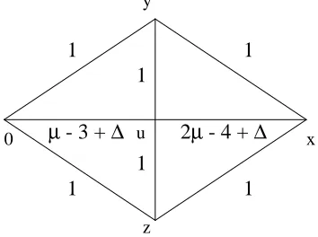
Figure 2: Basic three loop Feynman diagram.
of the tedious graphs in this respect is that illustrated in figure 2 where we have indicated the power of the propagator beside the line. We have used coordinate space representation where
one integrates over the location of the internal vertices,u,y andz, but withxcorresponding to
diagram of figure 3. There we have nullified the regularization since the associated factor from the transformation is
a6
(1)a(µ−3)a(2µ−4)
a(−1 + 2∆) , (53)
which, due to the denominator factor, is clearly divergent as ∆→ 0 sincea(α) = Γ(µ−α)/Γ(α).
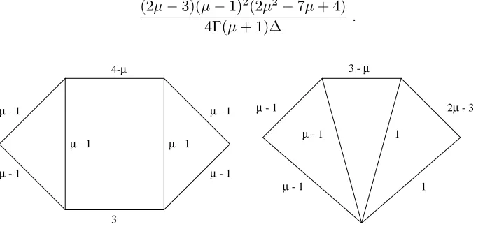
To proceed we use the language of [23] and apply a conformal transformation to the first diagram of figure 3 based on the left external point. Then integrating the unique triangle and subsequent unique vertex before undoing the original conformal transformation finally produces the second diagram of figure 3. The factor associated with these manipulations from the first diagram of
figure 3 is a4
(µ−1)/a(2µ−4). To deduce the value of the final diagram which is ∆-finite we
integrate by parts on the top right internal vertex based on the line with exponent 1. This produces four two loop diagrams. However, these intermediate diagrams are in fact divergent though their sum is finite. To ensure the correct finite part emerges, one introduces a temporary intermediate regularization prior to integrating by parts by shifting the exponent of the line
labeled 3−µ to an exponent of 3−µ+δ. In fact two of the resulting diagrams then cancel
exactly, leaving two integrals which are related to the function ChT(α, β) defined in [23] and
evaluated exactly in [31, 23]. Explicitly one has the difference of ChT(−1 −δ,3 −µ) and
ChT(µ−3−δ,3−µ) and expanding in powers of δ a finite expression emerges. Accumulating
all the contributions the final contribution of the integral of figure 2 to the critical exponent computation is
(2µ−3)(µ−1)2
(2µ2
−7µ+ 4)
4Γ(µ+ 1)∆ . (54)
µ - 1
µ - 1
µ - 1 4-µ
3
µ - 1
µ - 1
µ - 1
µ - 1
µ - 1
µ - 1 3 - µ
1
1
[image:11.612.122.467.356.520.2]2µ - 3
Figure 3: Intermediate three loop Feynman diagrams.
Having completed the computation of all the intermediate basic integrals we note that the
transverse contribution of each of the four diagrams of figure 1 toηO are respectively,
− (2µ−1)(2µ−3)CFη
o
1
2(µ−2)TF
, (2µ−1)(2µ−3)[CF − 1 2CA]η
o
1
2(µ−2)TF
,
(µ−1)2
CAηo1
(µ−2)TF
. (55)
Hence,
ηA2 = −
CAηo1
4(µ−2)TFNf
+ O 1
N2
f !
, (56)
in d-dimensions. Clearly this is equivalent to the sum of anomalous dimension parts of the
Landau gauge gluon and ghost critical exponents at O(1/Nf). More explicitly, from (48) and
(49),
which due to our choice of conventions and notation was the way this identity was originally uncovered in [6] prior to the all orders proof of [5] and its subsequent expression in the form
of (1). Therefore, (57) is an explicit d-dimensional verification of the all orders result of the
previous section. Moreover, it nicely recovers thed-dimensional case of [6, 5, 32].
As three dimensional QCD is of interest in other problems, we note that the explicit three
dimensional value of ωNATM is
ωNATM
d=3 =
1
2 −
4CA
3π2T
FNf
+ O 1
N2
f !
. (58)
In two dimensions, interestingly the critical exponent does not run to its mean field value and one has
ωNATM
d=2 = −
CA
16TFNf
+ O 1
N2
f !
. (59)
4
Generalization to other gauges: the example of the
Curci-Ferrari gauge.
The mass operator AaµAaµ in the Landau gauge can be generalized to other gauges, such as the
Curci-Ferrari and the maximal Abelian gauge. In this case the mixed gluon-ghost mass operator
1
2AaµAaµ+αcaca
has to be considered, whereαstands for the gauge parameter. Let us consider
here the case of the Curci-Ferrari nonlinear gauge. For the gauge fixed action we have
SCF =
Z d3x
− 1
4F
a
µνFµνa +ba∂µAaµ+ α
2b
aba+ca∂
µ(Dµc)a− α
2gf
abcbacbcc
− α
8g
2
fabcfcdecacbcdce+m2
1
2A
a
µAaµ+αcaca
. (60)
Notice that in this case also the Faddeev-Popov ghostsca,caare massive. Moreover, the
Curci-Ferrari gauge reduces to the Landau gauge in the limit α → 0. The action (60) is invariant
under the BRST andδ transformations of eqs.(5), (8). Introducing the external action
Sext =
Z
d3x−Ωaµ (Dµc)a+ La g
2f
abccbcc ,
it follows that the complete classical action
ΣCF = SCF+ Sext, (61)
turns out to be constrained by the Slavnov-Taylor identity
S(Σ) =
Z d3x
δΣ
δΩa µ
δΣ
δAa µ
+ δΣ
δLa δΣ
δca +b aδΣ
δca −m
2
caδΣ δba
= 0, (62)
and by the δ Ward identity
W(Σ) =
Z d3x
caδΣ
δca + δΣ
δLa δΣ
δba
= 0 . (63)
Due to the presence of the quartic ghost-antighost termg2
fabcfcdecacbcdceand ofgfabcbacbcc the
Proceeding as in the previous section, it turns out that the most general invariant counterterm
contains five free independent parameters, σ,a1,a2,a3,a5 and is given by
ΣcountCF =
Z d3x
−(σ+ 4a1)
4 F
a
µνFµνa +a1Fµνa ∂µAνa+ (a1−a2)ba∂µAaµ
+ a1(∂µ¯ca+ Ωaµ)∂µca+ (a1−a2)¯ca∂µ(Dµc)a+a5(∂µ¯ca+ Ωaµ)(Dµc)a
− a3
α
2b
aba+(a3+a5)
2 αgf
abcba¯cbcc+(a3+ 2a5)
8 αg
2
fabcfcde¯ca¯cbcdce
− a5
2gf
abcLacbcc+m2
(a1−
a2
2 +
a5
2 )A
a
µAaµ−αa3¯caca
. (64)
The parametersσ,a1,a2,a3,a5 are easily seen to correspond to a multiplicative renormalization
of the fields, sources and parameters, according to
Zg = 1−ησ
2 ,
ZA1/2 = 1 +ησ
2 +a1
,
Zc1/2 = Zc1/2 = 1−η
(a2+a5)
2
,
ZL = 1 +η
σ
2 +a2
,
Zα = 1 +η(−a3+ 2a2+σ) , (65)
and
ZΩ = ZA−1/2Z 1/2
c ZL, Zb1/2 = ZL−1 ,
Zm2 = Z− 2
L Z−
1
c . (66)
In particular, from eqs.(66) it follows that the renormalization factor Zm2 is not independent,
being expressed in terms of the ghost renormalization factorZc and of the renormalization factor
ZL of the source La coupled to the composite ghost operator 12gfabccbcc. Again, these results
are in complete agreement with those obtained in the four dimensional case [11].
5
Conclusion.
In this paper we have analysed the renormalization properties of the mass operatorAa
µAaµin three
dimensional Yang-Mills theories in the Landau gauge. In analogy with the four dimensional case,
the renormalization factor Zm2 is not an independent parameter of the theory, as expressed by
the relations (34) and (35), which have been explicitly verified in the largeNf expansion method.
These results will be used in order to investigate by analytical methods the possible formation of
the gauge condensate
AaµAaµ
. This would provide a dynamical generation of a parity preserving mass for the gluons in three dimensions, a topic which has been extensively investigated in recent years. For instance, see [33, 34, 35, 36].
Finally, we underline that the Curci-Ferrari gauge allows one to study the generalized mixed
gluon-ghost condensate 1
2AaµAaµ+αcaca
. In particular, as discussed in the four dimensional
case, the presence of the gauge parameterαcould be useful to investigate the gauge independence
Acknowledgments.
D. Dudal and S. P. Sorella are grateful to D. Anselmi for useful discussions. The Conselho
Nacional de Desenvolvimento Cient´ifico e Tecnol´ogico (CNPq-Brazil), the SR2-UERJ and the
Coordena¸c˜ao de Aperfei¸coamento de Pessoal de N´ıvel Superior (CAPES) are gratefully acknowl-edged for financial support. D. Dudal would like to acknowledge the warm hospitality at the Physics Institute of the UERJ, where part of this work was done. R. F. Sobreiro would like to thank the Department of Mathematical Physics and Astronomy of the Ghent University, where part of this work was completed.
References.
[1] H. Verschelde, K. Knecht, K. Van Acoleyen and M. Vanderkelen, Phys. Lett. B516(2001)
307.
[2] R. E. Browne and J. A. Gracey, JHEP0311 (2003) 029.
[3] K. Langfeld, H. Reinhardt and J. Gattnar, Nucl. Phys. B 621(2002) 131.
[4] A. C. Aguilar and A. A. Natale, hep-ph/0405024.
[5] D. Dudal, H. Verschelde and S. P. Sorella, Phys. Lett. B 555(2003) 126.
[6] J. A. Gracey, Phys. Lett. B 552(2003) 101.
[7] D. Dudal, H. Verschelde, V. E. R. Lemes, M. S. Sarandy, R. F. Sobreiro, S. P. Sorella and
J. A. Gracey, Phys. Lett. B574(2003) 325.
[8] D. Dudal, H. Verschelde, J. A. Gracey, V. E. R. Lemes, M. S. Sarandy, R. F. Sobreiro and
S. P. Sorella, JHEP0401 (2004) 044.
[9] K. I. Kondo, Phys. Lett. B 514(2001) 335.
[10] K. I. Kondo, T. Murakami, T. Shinohara and T. Imai, Phys. Rev. D 65(2002) 085034.
[11] D. Dudal, H. Verschelde, V. E. R. Lemes, M. S. Sarandy, R. F. Sobreiro, S. P. Sorella,
M. Picariello, J. A. Gracey, Phys. Lett. B569 (2003) 57.
[12] D. Dudal, H. Verschelde, V. E. R. Lemes, M. S. Sarandy, S. P. Sorella and M. Picariello,
Annals Phys.308(2003) 62.
[13] D. Dudal, J. A. Gracey, V. E. R. Lemes, M. S. Sarandy, R. F. Sobreiro, S. P. Sorella and H. Verschelde, hep-th/0406132.
[14] T. Appelquist and R. D. Pisarski, Phys. Rev. D23(1981) 2305.
[15] R. Jackiw and S. Templeton, Phys. Rev. D23(1981) 2291.
[16] S. Deser, R. Jackiw and S. Templeton, Annals Phys. 140 (1982) 372 [Erratum-ibid. 185
(1988 APNYA,281,409-449.2000) 406.1988 APNYA,281,409].
[17] F. Delduc and S. P. Sorella, Phys. Lett. B 231(1989) 408.
[18] D. Dudal, V. E. R. Lemes, M. S. Sarandy, S. P. Sorella and M. Picariello, JHEP 0212
[19] O. Piguet and S. P. Sorella, Lect. Notes Phys.M28(1995) 1.
[20] A. Blasi, O. Piguet and S. P. Sorella, Nucl. Phys. B356 (1991) 154.
[21] R. D. Pisarski and S. Rao, Phys. Rev. D32(1985) 2081.
[22] A. N. Vasiliev, Y. M. Pismak and Y. R. Honkonen, Theor. Math. Phys.46(1981) 104 [Teor.
Mat. Fiz. 46(1981) 157].
[23] A. N. Vasiliev, Y. M. Pismak and Y. R. Honkonen, Theor. Math. Phys.47(1981) 465 [Teor.
Mat. Fiz. 47(1981) 291].
[24] J. A. Gracey, J. Phys. A 24(1991) L431.
[25] J. A. Gracey, Nucl. Phys. B 414(1994) 614.
[26] J. A. Gracey, Phys. Lett. B 318(1993) 177.
[27] J. A. Gracey, Phys. Lett. B 373(1996) 178.
[28] O. V. Tarasov, A. A. Vladimirov and A. Y. Zharkov, Phys. Lett. B93(1980) 429.
[29] A. Hasenfratz and P. Hasenfratz, Phys. Lett. B297 (1992) 166.
[30] A. N. Vasiliev and M. Y. Nalimov, Theor. Math. Phys.55(1983) 423 [Teor. Mat. Fiz. 55
(1983) 163].
[31] K. G. Chetyrkin, A. L. Kataev and F. V. Tkachov, Nucl. Phys. B 174(1980) 345.
[32] K. G. Chetyrkin, hep-ph/0405193.
[33] D. Karabali and V. P. Nair, Nucl. Phys. B 464(1996) 135.
[34] D. Karabali and V. P. Nair, Phys. Lett. B 379 (1996) 141.
[35] R. Jackiw and S. Y. Pi, Phys. Lett. B 368(1996) 131.