Bioinformatics methods for
annotating genomes using
proteomic data
Abstract
Acknowledgements
The Biotechnology and Biological Science Research Council (BBSRC) that provided funding for this project.
I would like to thank my supervisor Andy Jones mentorship and the support from the members of my group that helped me throughout the challenges faced during this project.
BIOINFORMATICS METHODS FOR ANNOTATING GENOMES USING PROTEOMIC DATA ... 1-1
ABBREVIATIONS ... 1-1
1 INTRODUCTION ... 1-2
1.1
T
HEB
IOLOGICAL FRAMEWORK... 1-2
1.1.1 From DNA information to active proteins ... 1-2 1.1.2 Gene models ... 1-41.2
P
ROTEINS AND PROTEOMICS... 1-8
1.2.1 Protein modifications ... 1-8 1.2.2 Mass spectrometry proteomic workflow ... 1-11 1.2.3 Protein and peptide separation ... 1-13 1.2.4 Tandem Mass Spectrometry ... 1-151.3
B
IOINFORMATICS APPROACHES... 1-19
1.3.1 Database dependant approaches ... 1-22 1.3.2 Identification reliability: the assessed scores ... 1-26 1.3.3 De Novo sequencing and hybrid approaches ... 1-32 1.3.4 Explainable tandem mass spectra ... 1-341.4
P
ROTEOMICS AND PROTEOGENOMICS... 1-35
1.4.1 Proteomics challenges ... 1-35 1.4.2 Proteogenomics role ... 1-371.5
O
RGANISMS STUDIED... 1-39
1.6
R
ESEARCH OBJECTIVES... 1-41
2 GENE ANNOTATION: QUALITY ASSESSMENT AND
IMPROVEMENTS ... 2-43
2.1
A
BSTRACT... 2-43
2.2
I
NTRODUCTION... 2-44
2.3
M
ETHODS... 2-45
2.3.1 Understanding gene structure of studied organisms ... 2-45 2.3.2 Sequence database analysis ... 2-46 2.3.3 Alternative gene models ... 2-472.4.2 Defining the optimum length of ORF_SS ... 2-54 2.4.3 Datasets comparisons ... 2-56 2.4.4 Alternative gene models ... 2-67 2.4.5 Multiple database approach for official model evaluation ... 2-72
2.5
C
ONCLUSION... 2-83
3 INTRON SPANNING PEPTIDES: IDENTIFICATION BY A BLIND SEARCH STRATEGY ... 3-85
3.1
A
BSTRACT... 3-85
3.2
I
NTRODUCTION... 3-86
3.3
M
ETHODS... 3-87
3.3.1 Genome database TAGdb construction ... 3-92 3.3.2 Pipeline stage 1: from DB search to genomic regions ... 3-95 3.3.3 Pipeline stage 2: from InSPecT TAGs to spectrum anchors ... 3-98 3.3.4 Pipeline stage 3: from spectrum anchors to full length peptides ... 3-100 3.3.5 Pipeline stage 4: search engine against temporary database ... 3-104 3.3.6 Sample acquisition and test dataset ... 3-1043.4
R
ESULTS... 3-105
3.4.1 ISP identification by sequence database searches ... 3-105 3.4.2 Targeting ISPs: comparison of bioinformatic approaches ... 3-1083.5
C
ONCLUSION... 3-110
4 OPTIMISED BIOINFORMATIC PROCESSING OF N-TERMINAL
PROTEOMICS DATA: CHARACTERISATION OF THE N-TERMINOME OF
TOXOPLASMA GONDII ... 4-113
4.1
A
BSTRACT... 4-113
4.2
I
NTRODUCTION... 4-114
4.4
R
ESULTS... 4-127
4.4.1 How database design influences search engine performance ... 4-127 4.4.2 Analysis of the N-terminal Methionine ... 4-1364.5
C
ONCLUSION... 4-139
5 FINAL DISCUSSION ... 5-142
5.1
O
VERVIEW ON THE THESIS: ... 5-142
5.1.1 Achievements ... 5-142 5.1.2 Shortcomings ... 5-144 5.1.3 Framework for future developments ... 5-1455.2
P
ROTEOMICS:
WORK IN PROGRESS... 5-147
5.2.1 Latest advances ... 5-147 5.2.2 Future goals and challenges ... 5-147APPENDIX: A ... 5-149
6 ORIGINAL ISP PIPELINE DESIGN ... 6-149
6.1
M
ETHODS... 6-149
6.1.1 Original pipeline design: De Novo sequencing and sequence alignments for full-length peptide identification ... 6-149 6.1.2 Original pipeline design: performance evaluation of PepNovo ... 6-151 6.1.3 Original pipeline design: Sequence alignment ... 6-1526.2
R
ESULTS... 6-154
6.2.1 Original pipeline design: ... 6-1547 APPENDIX: B ... 7-158
Abbreviations
Hidden Markov model HMM
Stretch of DNA on the same frame comprised between 2
stop codons ORF_SS
Stretch of DNA on the same frame comprised between
Methionine and a stop codon ORF_MS
Short amino acid sequence TAG
Generic feature format GFF
Official gene model set OGM
Alternative gene model generated with GlimmerHMM GLM Alternative gene model generated with GeneMark gM Alternative gene model generated with FgeneSH FgSH Panel of gene model (official and alternative) P_GM
False discovery rate FDR
Short amino acid sequence tag TAG
Prefix Residue Mass PRM
Intron spanning peptide ISP
Whole genomic index based on 3 amino acid TAG TAGdb Coding sequences, stretches of DNA transcribed and
1
Introduction
1.1
The Biological framework
1.1.1 From DNA information to active proteins
Ever since the double helix structure of the Deoxyribonucleic acid (DNA) was elucidated in 1953 [1, 2] there have been enormous improvements in the understanding of the role of this molecule and how it relates to Ribonucleic acid (RNA) and proteins [3-5]. The basic structure of each strand of DNA is made by a long polymer of nucleotides linked together by a sugar molecule (2-deoxyribose) and phosphate molecules, which act as the backbone. This backbone, held together by asymmetric phosphodiester bonds, creates an inner direction of the polymer (5’ and 3’ prime ends, ending respectively with a phosphate and hydroxyl group). This leads to the assembly of a double helix, where opposite polymers are entwined together by interaction of the nucleobases (Guanine, Adenine, Thymine, Cytosine and Uracil [6-8]) as well as by hydrogen bonds. Each nucleobase from a strand binds specifically to a nucleobase of the opposite strand in a process called base pairing: Adenine (A) binds to Thymine (T), or Uracil (U) in RNAs, while Guanine (G) binds to Cytosine (C). In thermodynamic studies it has been observed that the stability of the double helix is directly affected by the G-C content, as their bond is stronger than A-T [9]. Unlike DNA, in the RNA chain, mostly single stranded [10], the alternative ribose molecule replaces the 2-deoxyribose sugar. Large DNA molecules (chromosomes) are made by millions of these repeated nucleotides; very large chromosomes can span from around 3x10⁷ to 9x10⁷ nucleotide repetitions such as chromosome 1 for Homo sapiens [11] and chromosome 3B of common wheat (Triticum aestivum) [12].
DNA-bound proteins are assembled as chromosomes, contained within the cell nucleus. The genes are mostly represented by non-contiguous fragmented stretches of DNA sequence. In prokaryotic unicellular organisms the nucleus is absent and the DNA, of circular structure, has higher gene density and less fragmentation [14-17].
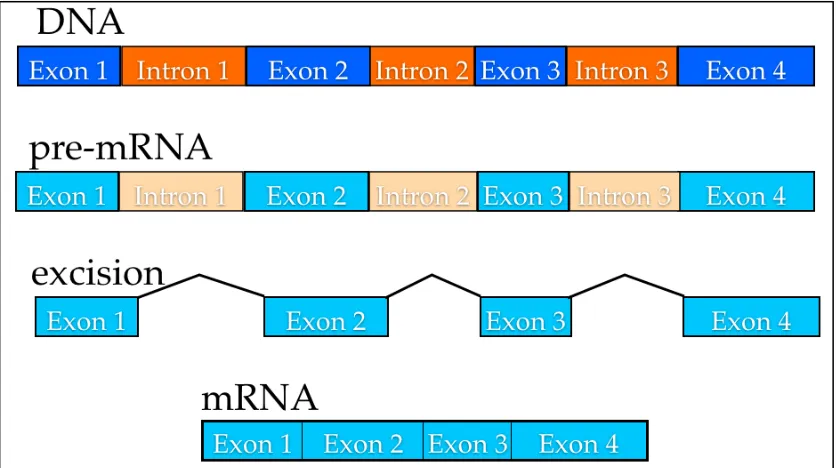
There are a large number of factors that influence gene expression such as non-coding RNA (transcriptional and translational), promoters and proteins. RNA-polymerases, which transcribe the gene sequences, also have the task of proofreading transcribed sequences preventing mutational errors [18-20]. The spliceosomes (large macromolecular complexes) remove the non-coding sequences located within the gene (introns) during the transcription from pre-RNA to messenger-pre-RNA [21, 22]. As the intron is excised at sites 3’ and 5’, the expressed sequences (exons) are joined together [21, 23-25] (Figure 1:1).
[image:11.595.84.504.374.608.2]
Figure 1:1 During transcription in eukaryotes, the non-coding introns regions are spliced out from the pre-mRNA and the resulting mRNA can then be translated by ribosomal RNA.
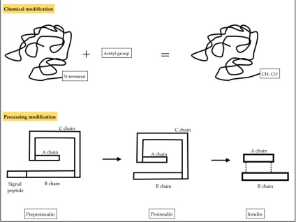
modifications have been found and they can be categorized into two groups depending i) whether they are formed by chemical linkage to the N or C terminal group or specific side chains, or ii) whether they are formed by processing, such as peptide segments removed by the protein chain (Figure 1:2).
Figure 1:2 Examples of chemical and processing modifications occurring in proteins. The chemical modification displayed involves binding of an acetyl group to the N-terminus (N-terminal acetylation), catalysed by N-(N-terminal acetyltransferase. The second modification shows the conversion of the precursor insulin protein preproinsulin into insulin. The signal peptide is cleaved after insertion in the endoplasmic reticulum; the protein then folds forming the C shape, proinsulin, allowing the A chain to bind to the B chain through disulphide bonds. The C chain is then cleaved leaving only the bound A-B chain, insulin, and thus activating the protein.
1.1.2 Gene models
of the regions encoding for proteins is performed with automated bioinformatic tools. In this thesis genome annotation is considered as determining the set of gene sequences predicted or confirmed for a given organism; the description of genes and their protein products represent instead the functional annotation. These are largely based on probabilistic interpretations and experimental data [26]. Widely available gene finder algorithms can be separated in two categories depending on which evidence is used for assessments: intrinsic and extrinsic.
both types of ORFs are used: Methionine_Stop (ORF_MS) and Stop_Stop (ORF_SS).
The second group include software packages like Genscan [44, 45] and Genewise [46]; these incorporate sequence alignments [47] from related species (using ESTs, cDNAs, RNA) in their predictions. However the gene models obtained with this method rely on the accuracy of previously curated gene models (for other organism); therefore these generated models are based only on the high ranked homologs, as weak homologs with different conserved regions would result in lower accuracy at exonic level [48].
Other ab initio gene finders such as Evigan [49] and Augustus [50-52], also allow the inclusion of data from external sources in the form of proteomic evidence and gene predictions from other software packages. These can provide useful as gene model predictions can be re-evaluated based on peptide sequences identified from the samples.
with the CDS. The start and the stop codons are represented by M and star symbols respectively. As illustrated, the start codon can appear within the coding sequences other than the first CDS as it codes for a common amino acid. Differently the stop codon only encodes for the end of translation and as such it cannot be contained within the coding sequences; as such it can appear within the gene region on frames other than the current coding sequence frame (e.g. here the first stop codon in frame one and two are both within the first exon boundaries). The open reading frames can be selected as sequences comprised by a start codon Methionine and a stop codon (ORF_MS) or between two stop codons (ORF_SS) on the same frame. Here the first frame has three ORF_SS and four ORF_MS as each start to stop codon are considered as ORF_MS (second and fourth ORF_MS are subsets of the first and third ORF_MS respectively). Without setting a minimum length threshold for ORF_SS it would be possible to include all exons; instead even if selecting all the possible ORF_MS it is possible to miss exons (i.e. here exon three and the exon five).
1.2
Proteins and proteomics
1.2.1 Protein modifications
Figure 1:4 The basic structure of amino acid molecules, showing N- C- terminal groups and the side chain. Through peptide bonding (Glycine and Alanine) water is released, keeping the same N- C- structure.
Through the reaction, the hydrogen molecule released from the amino group forms a molecule of water with the hydrogen and oxygen molecules from the carboxyl group. This process, also called condensation, can be reversed through the addition of water (hydrolysis) [55]. This is maintained throughout the length of the monomer chain where one end presents the NH2- amino group
modifications.
The signal peptide can be considered as a processing modification, which sees the amino terminal region of the protein cleaved off upon correct cellular localisation. Signal peptides are generally short sequences (~20-30 amino acid long in eukaryotes), positioned at the N-terminus, which serve as target signals within the cellular environment. Its structure comprises three regions: a positive charged n-terminus, a central hydrophobic region and a lightly polar c-terminal hydrophilic region [57, 58].
The signal peptide is present on secretory proteins and allows these to pass or attach to the ER membrane. The carboxyl region of signal peptides is detected by signal peptidase proteins, which perform the cleavage leading to the mature protein [59]. Different studies have investigated the role of the residue positions within the cleavage site, highlighting the importance of position -3 and -1 of the hydrophilic region as a pattern recognised by signal peptidases [60]. The most frequent residues at these positions have been identified as Alanine–x–Alanine [61].
The identification of signal peptides has been targeted with a number of computational tools (TargetP, SignalP, Signal-3L and Signal-CF [62-68]). These are generally based on a training set of known data and their algorithms include HMM models to identify secretory proteins and the cleavage site. Recent implementations have attempted to overcome the limitations in distinguishing between signal peptides and N-terminal helices of trans-membrane proteins (Phobius [69], Spoctopus[68], MEMSAT-SVM [70], SignalP4.0 [67]). In contrast to other software packages, SignalP4.0 is based on a neural network and works on two networks to assess the final score of cleavage positions (trans-membrane and non trans-membrane networks). However confident the predictions of signal peptides are, it remains a challenge to confirm these through proteomic analysis.
process it appears that the amino acids following methionine may affect whether the cleavage takes place [71]. Other cleavages simply allow the protein to change state until needed (e.g. signal peptide cleavage and self-splicing synthesize insulin protein from its preproinsulin precursor, Figure 1:2).
Through reversible and non-reversible chemical modifications protein activity can adapt and respond to external stimuli. Important for energy transfer and signalling within the cell, phosphorylation (a phosphate group bound to Serine, Threonine, Tyrosine and Histidine by protein kinases) can be frequently observed within the proteome, and for each protein this multi-site modification can be potentially performed and reversed several times [72]. Equally important is the reversible modification involving the addition of the acetyl group to the N-terminus (by N-terminal acetyltransferase proteins), which affects gene regulation and is also frequent [73-78].
Other common modifications include glycosylation [79-81] (oligosaccharide group added to secretory/membrane proteins), methylation [82-84] (chemical link on side chain specific residues Lysine and Arginine [85]) and ubiquitination [86-88] (protein degradation performed by ubiquitin activated enzymes).
The large number of all possible modifications for each protein on the whole proteome scale makes protein prediction and the annotation process increasingly challenging.
1.2.2 Mass spectrometry proteomic workflow
Mass spectrometry (MS) based proteomic studies (Figure 1:5) offer a way to annotate the genes by allowing the annotator to validate the presence of the proteins in a sample [89] in a quantitative or qualitative manner [85].
these can be further fragmented into smaller ions during a two-stage analysis in a Tandem Mass Spectrometer (MS/MS).
The peptides can either be obtained by separation of a digested protein mixture, as in Multidimensional Protein Identification Technology (MudPIT) [90, 91], or for example by in-gel digestion after electrophoretic separation of proteins [92]. This approach for protein identification is also known as bottom-up proteomics. In order to draft the peptide results to list proteins as identified (procedure also referred to as protein inference) it is necessary to assemble these resulting peptides and assess their confidence. To draft this list of peptides considered as reliable one must also consider whether the peptide is contained in multiple protein sequences, or whether only one peptide per protein was identified (problem known as “one-hit-wonder”) [93]. In this stud the protein inference step y makes use of these considerations and as such the proteins here identified must contain one unique peptide to be considered confident identifications.
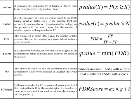
However as statistical methods are used to computationally assess the significance of spectral interpretations, it becomes challenging to validate the correctness of the interpreted sequence within very large datasets [94]. With generally adopted database search approaches the statistical importance of the identifications are given as the probability that each one is incorrect such as p-value estimate. This can be seen as the probability distribution that a null hypothesis is true, such as that a peptide spectrum match (PSM) with the same or better score happens by chance in a sequence database [95, 96].
Figure 1:5 Basic proteomic workflow divided in 3 main stages: biological sample preparation (orange) where the sample goes through subcellular fractionation (a), protein separation (b) followed by proteases (c), resulting in peptide mixtures (d). During mass spectrometry stage (green) these peptide mixtures are further separated through the Liquid Chromatography (a); ionised peptides are detected (b) and selected peptide ions are fragmented (c) resulting in tandem mass spectra. Finally, during bioinformatic analyses (blue), the obtained spectral data (a) is processed with (b) specific software packages that identify (c) the peptide spectrum matches (PSMs) and provide protein inference (d).
1.2.3 Protein and peptide separation
The process of 2-DE addresses this limitation by separating the molecules first by their net charge, isoelectric focusing (IEF), and then by their MW. This separation over 2 different axes achieves a higher resolution [92, 99]. This process has clear advantages like resolving thousands of proteins at the same time on a single 2-DE gel as well as separating/ revealing proteins with PTMs. There are some limitations associated with this method as proteins of very large or small size. Also hydrophobic proteins such as membrane proteins are generally difficult to observe in 2-DE gels. It may be difficult to detect low abundance proteins with conventional staining although protein pre-fractionation preceding 2-DE can simplify protein mixture [100]. Figure 1:6 taken from Xia et al. [101] paper, shows a 2-DE gel with localized spots.
Figure 1:6 Example of a 2DE gel electrophoresis. This has been obtained from T.gondii for proteomic annotation in the Xia. et al study [101].
carboxyl end of arginine and lysine amino acids as long as these are not followed by proline [102].
Prior to mass spectrometry, High Performance Liquid Chromatography (HPLC [103]) is often performed, which makes use of the different hydrophobicity of the peptides to perform the separation.
1.2.4 Tandem Mass Spectrometry
The prepared samples are then ready to be analysed in the Mass Spectrometer and the analysis is performed in 3 phases (Figure 1:5):
• the samples are firstly ionized (using for example MALDI (described below) [104] or Electrospray [103]);
• the ions are then separated (Time-of-flight, Ion trap, Triple quadrupole [105]);
• and finally the ions are detected;
Peptide ionisation is mainly performed with Matrix Assisted Laser Desorption Ionisation (MALDI [104]) and electrospray ionisation (ESI [103]). The first technique uses a laser and a light absorbing matrix to desorb and ionise the molecules, generating mainly singly/ doubly charged ions. The second technique involves molecules going through a capillary tube contained within an electric field, generating mainly multiply charged ions. By identifying C-12 peaks
and using mono-isotopic masses it is possible to calculate the charge of the ion and peptide mass.
These peptide ions, confined by an electric field, are separated and detected based on their mass-per-charge (m/z) ratio during the MS1 pass. Then the most abundant ion species can be selected to go through further fragmentation into smaller ions (in data dependent acquisition instruments), which are then detected in the MS2 stage, from which peptide sequence information can be derived (Figure 1:5).
The peptide fragmentation can be obtained with different techniques, such as Collisional Induced/Activation Dissociation (CID, CAD [114]) or Electron Transfer Dissociation (ETD) and Electron Capture Dissociation (ECD [115]). Each technique produces predominant ion series (Figure 1:7) from peptide bond fragmentation (i.e. CAD leads to -b and -y ions while ETD and ECD lead to -c
Figure 1:7 Tandem MS spectrum from a peptide, TMEEFVIDLLR, identified by the y- ion ladder (MASCOT).
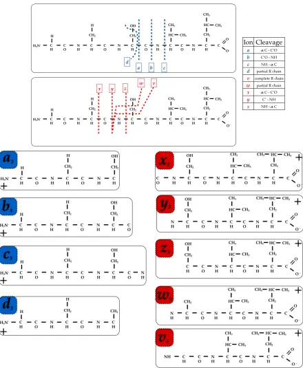
If the fragments do not carry any charge they would simply not be detected. Fragment ions (Figure 1:9) resulting from backbone cleavage either at alpha C-CH, C-N or N-αC are usually indicated with a, b or c if the charge is retained on the N-terminus; instead if the charge is retained on the C-terminus they are indicated with x, y or z (with a subscript indicating how many residues in the fragment). Also present, but not commonly observed as high CID is required, are
d-v- and w- ions, resulting from side-chain cleavages.
1.3
Bioinformatics approaches
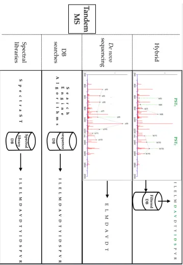
In bottom-up mass spectrometry proteomic experiments the peptide sequences can be interpreted by different bioinformatics approaches (Figure 1:9). In sequence database searches experimental mass spectra are compared against theoretical fragmented spectra generated by computationally digested protein sequences or six-frame translations [117-123]; the result is a statistically significant identification for a proportion of the collected mass spectra. de novo
sequencing instead attempts, through probabilistic networks and complex algorithms, to interpret the peptide sequence yielding the spectrum with no previous knowledge of the sequence [124-126]. Hybrid methods combine de novo
and sequence database search in two steps: initially, computational algorithms provide sets of short amino acid, called TAGs, yielding adjacent peaks in the spectrum, then with this information the algorithms filter the sequence databases and perform database searches on a generated, restricted database [127-130]. In the spectral library search approach, unknown spectra are identified through comparison against compiled database of spectra. In this case the database/ library holds a large collection of observed high-quality spectra with identified peptide sequence [131, 132].
used for identification.
1.3.1 Database dependant approaches
The workflow for the first type of approach, typified by the MASCOT search engine [122], is as follows. MASCOT allows both Peptide Mass Fingerprint (PMF [135]) as well as an “MS/MS Ion Search”. PMF is used to identify proteins by matching their constituent peptides masses (MS1 only) to the theoretical peptide masses generated from a protein database. The PMF identifications rely on observing a large number of peptides from the same protein at high mass accuracy. It is better used together with 2-DE data where proteins are generally separated into simple mixtures [136].
The MS/MS technique can be used to identify a protein from even a single peptide, even though the quality of the result will increase by searching an MS/MS run containing several peptides for a given protein. In the MS/MS search the experimental spectra are used to gather information about the precursor ion masses. In Sequest [119, 123, 137, 138] both experimental and theoretical spectrum are pre-processed where normalization of signal intensities allow the spectra to be comparable. In OMSSA [120] there is no normalization process but instead noise removal.
The sequence database is processed and the search engine generates a set of theoretical spectra for all digested peptide sequences, whose mass falls within the mass tolerance. It then proceeds by fragmenting each sequence in this temporary set by recreating in silico fragmentation for each ion (a, b, c, x, y, -z). Finally it tries to match each expected value against the experimental value in the original spectrum. Each ion is given a score and all positive matches, within the tolerance window, between the theoretical spectrum and experimental are summed in the final score of the reconstructed the peptide sequence.
commercial software package distributed by GeneBio, Geneva Bioinformatics SA, has a two-step analysis for searching combinatorial modifications and an algorithm to evaluate which of the alternative matches is most probable [121, 141, 142].
MASCOT provides a statistical weighting for each individual PSM, based on the quality of the match between experimental and theoretical spectrum. This probabilistic approach is based on the MOWSE (for MOlecular Weight Search) algorithm [122, 143].
Figure 1:10 MASCOT result summary view:
A: Rank of identified protein sequences by the sum of their peptide score;
B: This is the accession number of the sequence (computationally predicted Open Reading Frame in this case) and the peptides matched against. It leads to another page containing the full sequence and showing how peptides align to it.
C: Expected mass of the protein/sequence in Daltons.
D: The protein score is approximately the sum of each individual peptide score, derived from ion score
E: The number of MS/MS spectra matched
F: The identifier of the query matched against the peptide, it leads to a page with full Peptide view of the spectrum identifier.
G: This is a summary of peptide different mass/per charge, which provides the observed mass queried against its theoretical uncharged mass, the theoretical closest peptide mass matched and their difference.
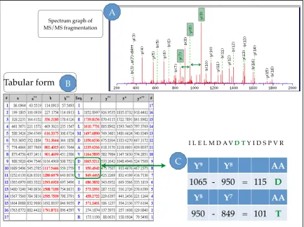
Figure 1:12 The arrows shows how the spectrum graph (A) and the tabular form (B) can be traced back to the peptide sequence (C) ILELMDAVDTYIDSPVR.
A: From the theoretical fragmentation in the spectrum graph it is possible to view peaks –y7, – y8 and –y9.which allow identifying consecutive amino acids D and T.
B: The tabular form for these fragmented ions shows the matches in BOLD RED for each ion type.
C: Highlighted in green is an example of how each amino acid residue can be calculated based on the difference between adjacent ion fragment masses.
1.3.2 Identification reliability: the assessed scores
in other words, a p-value assigned to a PSM A describes the probability of seeing a PSM B with the same or better score of A if B has been matched by random chance. In proteomic studies it is not uncommon for thousands of spectra to be searched against sequence database and this leads to the need to correct the score for multiple testing. The e-value, similarly to Bonferroni correction, provides multiple testing correction and it is defined as the expected frequency of PSMs having a better or equal score assuming that they have been matched to a given spectrum randomly [145]. It is calculated using the p-value and the search space, number of spectra and database length (the number of peptides, that are contained within the chosen tolerance, from the database); as an example the MASCOT [122] ion score is calculated from the probability P that the observed match is random event and it is reported as −10log𝑃.
Nesvizhskii et al [146] observe that the score distribution for each tool is influenced by many factors such as the quality of the mass spectrometer, the data and the database size. Hence by assessing the false discovery rate (FDR) [147] it can be possible to overcome these limitations [148]. The search engine results are re-scored using the FDR-based statistical methods to validate the expected rate of true positives and false positives of PSMs present below a FDR cut-off score. For this method, the original queried databases contain also a decoy set, sequences that are known to be incorrect. There are different methods to generate these sequences: generally the protein sequences are reversed, or the tryptic sites are conserved while the amino acids are shuffled in order. Then this can be interpreted as a binary classification problem in which a hypothesis can either be True (T) or False (F) and their results can either be Positive (P) or Negative (N), leading to 4 possible outcome, as shown on the table in Table 1:1.
True actual value False actual value Predicted positive
outcome True positive (TP) False Positive (FP) Predicted negative
outcome False negative (FN) True negative (TN)
From a real true result, if the outcome is also positive, then we can consider it as TP (true positive) while if the outcome is negative it will be a FN (false negative); while in the case of an incorrect (false) actual value, like a decoy sequence for instance, the results can be scored as either positive (FP) or negative (TN).
The equation for the global FDR algorithm used in this thesis is the following:
𝐹𝐷𝑅 = 𝐹𝑃 𝑇𝑃+𝐹𝑃
Where the FP (false positives) value is estimated within PSMs by counting the number of “decoy” PSMs above threshold. The TP (true positives) are calculated as 𝑇𝑃 = 𝑇−𝐹𝑃 where T comprises all PSMs above threshold [148].
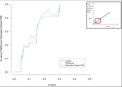
[image:36.595.86.512.352.655.2]As a practical example, in a dataset, the search engine score such as the e-value is used to sort the PSMs; then, going from the lowest to the highest value, the PSMs are then labelled as FP if they are from the “decoys” otherwise they are calculated as TP (𝑇𝑃 = 𝑇−𝐹𝑃 ); then the FDR is then calculated for each identification. As an example, considering a dataset of 100 PSMs above given FDR threshold, if 5 PSMs came from the decoy database it will lead to a total number of 𝐹𝑃 = 5, while the 𝑇𝑃 = 90; that is within the 95 target PSMs there will be approximately 5 false positives thus 𝐹𝐷𝑅 =!"!. The total number of TP can then be obtained through a fixed FDR, normally 1% or 5%.
In addition to FDR is the Posterior Error Probability (PEP), sometimes denoted as local FDR [150]. This assesses the probability that the null hypothesis is null and as such that the observed PSM is incorrect [151] (Figure 1:14). As illustrated by Kall et al the non-parametric approach for calculating the PEP for a given PSM can be affected by the bin size by which the target and decoy PSMs have been divided. There have been other developed algorithms for calculating the PEP such as PeptideProphet [152, 153] and Percolator [154].
Figure 1:14 The FDR and PEP scoring curves drawn in the study by Käll et all [145] visualise the area (A and B) and the heights of the distribution. The FDR is the ratio of the incorrect PSMs with score > x (B) to all PSMs (A+B) score > x. The PEP is the ratio of the heights of distribution at score = x where b is the incorrect PSMs at score = x while a is the number of correct PSM with the same score x.
six-frame translations [157]. Compared to searches against gene annotations, searching 6 frame translations appears to be biased. This is due to the presence of 6 (incorrect) frames (from the decoys) added to the 5 alternative (also incorrect) frames, competing against a single correct frame. Additionally it should be stressed the importance of choosing the correct score. Given its properties the global FDR and q-value are rates related to the whole dataset and as such useful when analysing multiple identification within the dataset. However when the analysis is focused on assessing the reliability of one precise identification, then PEP should be chosen as it provides the probability that given identification is incorrect (Table 1:2).
1.3.3 De Novo sequencing and hybrid approaches
As explained previously, de novo sequencing algorithms can provide useful information for unanticipated peptide sequences [158, 159], but they are still limited to very short sequences of amino acids identified with high confidence in the mass spectra. Key to de novo reconstruction is the score or probability assigned to peptide sequences such that the highest score reflects the best out of all interpreted peptide sequences [160, 161].
Some scoring algorithms are based on the correlation between observed and theoretical spectrum obtained from candidate peptides. Others evaluate the score from observed peaks by comparing statistical models based on ion fragmentation rules and against fragmentations led by a random process (Figure 1:15) [125]. This is however computationally difficult as the probabilistic distribution appears too complex to be modelled and often leads to errors [162-165].
The de novo sequencing software PepNovo [161, 166, 167], like InSPecT (Interpretation of Spectra with PT modifications) software (Figure 1:16), initially analyses the mass spectrum to identify peptide sequence tags (PSTs), short amino acid sequences, and then attempts a full peptide sequence reconstruction. The InSPecT algorithm computes the score from three factors: intensity rank of the peak, isotope pattern and prefix residue mass (PRM) that represent each node from the constructed directed acyclic graph. By default the output is a set of long amino acid sequence, where the high confidence PST is contained. PepNovo algorithms are currently based on a training dataset obtained from mass spectra where the fragment ion has been achieved with collision-induced dissociation (CID).
Figure 1:16 Peptide identified with InSPecT as database search engine. In this mode, its algorithm first generates a set of interpretations for high intensity peaks and from these it reconstructs peptide spectrum tags PSTs (typical length of three amino acid). The spectrum above shows DAV and IDS as calculated PSTs. Exploiting the TAG pattern and the spectrum mass the sequence database is filtered. Finally a search database query is performed on this restricted database.
Most of the de novo sequencing software packages try to overcome the limitations in accuracy by combining analysis with search databases e.g. used in InSPecT, PEAKS and SPIDER, MS-Dictionary [127, 160, 168-171]. The approach comprises
their prefix and suffix m/z value (corresponding to -b and -y ions) [170]; this allows them to place the TAG (Figure 1:16) within the spectrum and with this information the sequence database is filtered in order to maximize peptide discovery of unknown sequences while querying a large starting sequence database [171].
1.3.4 Explainable tandem mass spectra
sequencing) where at best removing around 80% of unworthy spectra leads to a 10% loss of explainable spectra [177].
1.4
Proteomics and proteogenomics
1.4.1 Proteomics challenges
Bottom-up proteomics approaches use digested protein sequences for identification. The confidence of protein identification is connected to the number of peptides that were used to identify the protein. The identification of low abundance peptide sequences and the presence of post-translational modifications (PTMs) can prove challenging for proteomic studies. In recent years mass spectrometry proteomic studies have increasingly provided researchers with a high-throughput method for identifying and measuring proteins, targeting their interactions, post translational modification and for annotating genes [123, 138, 178-180].
Unlike prokaryotes, which feature compact genomes with only a small amount of non-coding sequences outside and within gene boundaries, eukaryote genomes present a far more complex structure where genes contain a large number of sequences that are removed between pre-mRNA and mRNA (Figure 1:1). Ever since spliced genes were found, the presence of intragenic regions was considered of particular biological importance, for example as a driver of evolution [181].
Since multiple-exon genes in eukaryotes can be translated into more than one protein product due to alternative splicing, it is crucial to correctly predict intron-exon boundaries [21, 25, 182, 183].
it is still a huge challenge to find these peptides with bioinformatics approaches as they partly rely on gene finder accuracy. If the gene finders have not predicted the correct splice junction of a gene, it will not be possible to identify the spectra of intron-spanning peptides (ISPs) during analysis on the sequence.
No matter how accurate gene prediction software can be, it is not unusual for them to miss out short single exon genes [184], or fail to detect different protein isoforms due to alternative splice sites [185-187]. If, for example, the mean length of each exon in a multi-exonic gene is about 50 amino acids there is a 25% probability that a tryptic peptide is crossing intronic boundaries [188]. EST approaches such as the Transcript Assemble Program (TAP) [189] have been implemented in order to maximize the identification accuracy of splice variants generating results with good sensitivity. However it remains intrinsically dependent on EST coverage [190] which is often low.
Although a multiple database search approach such as querying Open Reading Frames (ORF_SS) or panels of alternative gene predictions can assist at correcting/ confirming annotation [178, 194, 195] (Figure 1:17), the approach would still be dependent on a protein/peptide sequence being present in the database. Even to this day, it remains a bioinformatic challenge to provide proteomic evidence of intron exon boundaries; the so-called splice sites or splice junctions [196-198], since confirming the presence of these elusive peptides in the experimental data relies on accurately predicted protein sequence [101, 188, 199-201].
Also challenging are the N-terminal peptides, due to possible N-terminal modifications (i.e. signal peptide) and bioinformatic difficulties in correctly predicting the translational start of the protein.
1.4.2 Proteogenomics role
In the recent years mass spectrometry-based proteomics have advanced considerably providing rapidly improving techniques for generating comprehensive collections of data from studied organisms. Dedicated sample preparation (fractionation protocols and multiple proteases) makes it possible to increase depth in sub-cellular proteome analyses and expand sequence coverage [202]. With an ever-increasing number of genome sequencing project throughout the scientific community, thousands of genome sequences are now available for deeper proteomic research studies. Publicly available resources such as Genome Online Database (GOLD [203]) provide an outlook on genome sequencing project across the world.
Adamini et al, attempts to combine shotgun proteomic evidence with de novo
transcriptome sequencing [205] to confirm expressed protein-coding genes for S. mediterranea. Through a comparison of identified tandem mass spectra (<1% FDR) on an available gene model set and their sequenced transcriptome, they highlight the importance of proteomic evidence for validating previous gene models [206, 207]
Proteogenomic studies are closing the gap between proteomics and genomics, providing gene annotators with tandem mass spectra-derived peptide evidence for protein identification and characterization. In this study Castellana et al [208] refine the A. thaliana proteome by querying 3D LC tandem mass spectra with InSPecT search engine [171] against 3 distinct sequence databases: official proteome (TAIR), 6 frame translation and a splice graph (for all putative splice events). By providing proteomic evidence for ~12k genes, identifying ~500 novel genes and refining around 1000 gene sequences they bring support to proteogenomics approaches. The lack of data for low abundance proteins in the sample and low quality tandem mass spectra can be seen as limitations to their approach.
In another interesting proteogenomic approach developed by the same group an imperfect genomic template is exploited with tandem mass spectra to successfully return the correct target protein [209]. Here spectra are used to construct the template sequence, where their chain order is given by the genomic sequence (6 frame translation of gene loci). Then anchors are selected by overlapping spectra providing specific amino acid substrings that appear with no mutations on both template and target proteins. The final stage of their method sees the extension of these anchors to create the protein sequence. However this method is still limited by both PTMs and unexpected splice sites present in the sample, as the consensus algorithm would miss these out.
studied species; it is also based on highly curated genomes to assess identification of the sequence on less curated genomes. Rare unexpected modifications require further evaluation in order to measure their confidence.
Proteomic data can help to confirm not only the presence of gene expression as well as PTMs but also the complex structure of genes [171, 209] and protein-protein interactions [211]. This data has been already exploited for genome annotation of several organisms such as Toxoplasma gondii [101], Plasmodium falciparum [212], Drosophila melanogaster [213], Homo sapiens [214] and
Caenorhabditis elegans[178].
1.5
Organisms studied
The Apicomplexan parasites are responsible for major tropical diseases such as Malaria caused by the plasmodium parasite, alone responsible for hundreds of thousands of cases resulting in death worldwide [217-221]. Toxoplasma gondii, the most common zoonotic parasite, can infect all warm-blooded animals and around the globe more than a billion people are infected [222]. This, among other coccidia, is one of the most extensively studied [223] with several genomes sequenced to this day [224]. Neospora caninum, closely related to toxoplasma, causes abortion in cattle. It can be transmitted horizontally and vertically, where it can pass consecutively and intermittently to the offspring [225, 226].
Notably, there are genomic structural differences across the eukaryotic parasites of the phylum Apicomplexa such as Cryptosporidium parvum, Plasmodium falciparum, Toxoplasma gondii and Neospora caninum [42, 193, 227-229], which are studied in this work. Compared to the P. falciparum genome, the C. parvum
genome appears to be almost two fifths smaller and presents an almost doubled gene density. This divergence increases with the T. gondii genome, which, with its 14 chromosomes, is over double in size compared to P. falciparum and presents a lower gene density having more introns per gene [230-232].
As currently genome annotation is largely based on predictions of the gene structures, these can dramatically change over time as more accurate predictions are computed and released to the public [184]. Using sequence databases such as UniProtKB, NCBIgi and IPI can lead to out-dated peptide sequences reported in their protein identifications from proteomic studies [233]. Even in a well-annotated genome there is a large percentage of hypothetical proteins (purely based on predictions and without known domains) and putative proteins (having sequence similarity with characterized proteins but not experimentally validated) [234]. As an example, during evaluation on the genome structure of apicomplexan parasites, P. falciparum presented only ~0.68% hypothetical and ~32% putative, while for C. parvum, N. caninum and T. gondii were respectively ~40% and ~5%, ~43% and ~33%, ~64% and ~31% [101, 227, 232, 235].
The data for this project, used for mining or statistical evaluation, comes from:
Neospora caninum (Table 1:3).
In the recent years genome sequencing has been performed for these species. In this project, due to the close evolutionary distance, I have been using Toxoplasma gondii to provide a statistical insight on the current quality of annotation for the later sequenced Neospora caninum genome and how it could be improved (Table 1:3 [193, 227-229, 231, 236-238] - for further sources EupathDB).
Table 1:3 Genome sequence and proteomic data available for apicomplexan parasites. It takes consideration of the recent annotation improvements of N. caninum [239].
1.6
Research objectives
multi-sequence database approach is devised, similar to a multiple search engine mode, to examine the performance of specific database structures (e.g. gene models, six frame translation or ORF_SS/ ORF_MS). This analysis can be used to improve current database structure resulting in increased peptide identification. This type of approach is then tested on past and presently available genome sequences for T. gondii and N. caninum to provide a broad picture of genome annotation progress through time.
Furthermore the research focuses on targeted peptide identification to confirm and correct gene structure as well as novel identifications. The peptide sequences in question are those peptides that span across two exons and N-terminal peptides. As only querying gene models can confidently identify the first type, a novel type of method is proposed. This method can be considered as a type of hybrid approach, involving peptide sequence tag identification and database searches; but the result is similar to a de novo approach since it works in the absence of gene models for full-length peptide identification.
2
Gene
annotation:
quality
assessment
and
improvements
2.1
Abstract
As most current gene annotations only result from computational predictions, proteomic data can be used to assess and validate them. This chapter proposes database design strategies to address limitations in both assessments of draft annotations and maximisation of peptide identification from tandem mass spectra. The designed strategy comprises multiple database searches followed by analyses and comparisons of the datasets searched against different databases.
The pipeline compares results from official gene models and open reading frames (ORFs) derived from a six-frame translation, and identifies PSMs that are unique to individual databases for further investigation. This gives an overview on database performances (i.e. gene model accuracy).
2.2
Introduction
Genome curation is generally performed with automated methods [28-30, 49, 51] and it undergoes multiple refinement stage before an annotation is considered as complete. Although proteomic studies enable protein identification based on draft annotations it remains uncertain how to assess the accuracy of these predicted models. Recent bioinformatics improvements have provided increased confidence in the peptide sequences identified with search engines [118, 119, 122, 148, 168, 171, 188, 234, 240-242]. This facilitates searches for novel genes and corrections on genomic structure through genome wide searches. Since open reading frame sequence databases (ORFs) are generally used for genome-wide database queries the strategies discussed in this chapter comprise analyses to improve ORF prediction for search optimisation [243].
At the time this study was started, the Sanger Institute had recently released the
N. caninum genomic sequence and highly annotated gene models were available (release 5.0) from the closely related T.gondii ME49 [101, 230, 239, 244, 245]. Because of the evolutionary similarities the T.gondii annotation was used to provide an initial assessment of N. caninum gene models. This enabled the hypothesis to be formulated that N. caninum annotation could be improved, since the model was missing out ~2K genes. Through further rounds of annotation at the Sanger Institute [239] we were later provided with more accurate N. caninum data to test the theory.
One of the objectives here discussed is how ORF_SS prediction could be improved to yield the best set of sequences while improving search performance. This was achieved by evaluating the genomic structure of other apicomplexan organisms: C. parvum, P. falciparum and T. gondii [42, 193, 227-231, 246].
The designed pipeline enables us to compare the PSMs in the datasets and generate Venn diagrams. By tracking PSMs back to specific sequence databases, this can facilitate further design refinements. This approach was used with ORF_SS and gene model databases to adjust the predicted model. Additionally this method proved useful as part of a new protocol for accuracy assessment of gene models using proteomic data.
The multiple database study also included assessment of multiple search engines performance compared to individual search engines. By incorporating alternative gene models in the study it was also possible to highlight their importance in a proteogenomics context; it also showed a rough benchmark of Glimmer and GeneMark software packages.
This chapter has the following aims:
• to improve the design of ORF_SS databases;
• to provide additional evidence for N. caninum annotation improvements; • to measure the improvements of the gene models over time;
• to benchmark gene finding software and the multiple search engine approach;
2.3
Methods
2.3.1 Understanding gene structure of studied organisms
achieved by extracting the putative Open Reading Frame (ORF) sequences [243, 247, 248]. The ORF sequences discussed in this chapter are those stretches of sequence, located on the same reading frame, comprised between two stop codons (ORF_SS as referred to in the introduction chapter).
In order to generate an ORF_SS database containing relevant data, while filtering out likely non-coding regions, it is necessary acquire some statistical figures on the genomic structure of the organism analysed. The initial study comprised the annotation release 5.1 for Neospora caninum as well as Toxoplasma gondii release 5.1 and other species from the same phylum for which the annotation is at a more advanced stage such as Cryptosporidiumparvum and Plasmodium falciparum
release 4.1 and 5.5 respectively. The last two organisms were selected to validate the statistical methods used for analysing the others.
2.3.2 Sequence database analysis
The workflow for the database searches and scoring approach was designed to include a False Discovery Rate assessment algorithm [148]. As such, to construct the decoy sequence database the original sequences were reversed with a flag in their accessions (i.e. the word “Rev” prefixed to all headers); this was then concatenated to the original sequence database.
The database search engine software of choice for analysing MS/MS data was X!Tandem [140] and MASCOT [122]. The searches with MASCOT were performed considering: peptide charge of 1+, 2+ and 3+, trypsin digestion, fixed modifications of carbamidomethyl on cysteine and methionine oxidation allowing only 1 missed cleavage, with MS peptide and MS/MS tolerance of ±0.8 Da, after having tested various alternatives, to maximize output at fixed FDR (Appendix B Figure 7:1).
N.caninum 5.1 sequence databases: ORF_SS provided by EupathDB.org, ORF_SS with threshold length of 40 amino acids and the official gene annotation, respectively (see Appendix B Figure 7:1). This method can facilitate the evaluation of sequence database design and optimisation of search parameters.
2.3.3 Alternative gene models
The gene finder software packages used include GlimmerHMM [28, 29, 39] and GeneMark [30, 31, 249]. GlimmerHMM is fully configurable for new organisms, since with enough genomic data it is possible to create new HMM trained models.
Whenever possible only coding sequences from the available gene model were used to generate new GlimmerHMM models. The theory was based on the relation between training data accuracy and HMM model optimisation. For historical evaluation of the official gene models accuracy GlimmerHMM models have been generated using the previously available official release. When the trained models were created with the purpose of contributing to the current annotation, the official model from the same release was used as source data.
For both software packages only default parameters were used, without altering the values for isochores (stretches of genomic sequence with higher content of GC). This was decided as the overall GC abundance throughout the different chromosomes demonstrated little variance across the T.gondii genome. In
T.gondii the difference of GC frequency between coding and non-coding regions is very small and not evident.
slow searches for no gains in PSMs (data not shown). The results showed a general consensus in exon predictions across the top ranking predicted models; instead different ranks are directly connected to the way the exons are assembled into genes (the predicted splicing of exons).
GeneMark does not require previous training for a specific organism for the assessment of hidden states during HMM predictive algorithm. This software package has been designed with Viterbi Algorithm [30, 37] that generates a variable number of hidden states as needed during the computation of gene predictions.
For each species all available sequenced genome releases with their respective official gene model were gathered whenever there was a change between releases. In the case of T.gondii the whole shotgun genome sequences were available for the releases: 3.3, 4.x, 5.x and 6.x. The gene models came instead from only three releases: 3.3, 4.x, 5.x (5.x was unchanged in 6.x and 7.x) [250]. The first publicly available gene model, release 3.3, was generated using different gene finding software: Glimmer, Tigrscan (ab initio) and Twinscan (ab initio and homolog alignments). The second available release for gene model 4.3 was generated by GLEANS, incorporating EST data. To generate predictions for
N.caninum we used the genomic sequence and models 5.x and 6.x available from EuPathDB. The pre-release 7.x of T. gondii was evaluated for additional updates/ changes, but there were none.
2.4
Results
2.4.1 Gene structure of the Apicomplexa
The figures needed to assess the genomic structure were the distribution of lengths of the genes and the length of their initial, internal and final exons. To provide a visual comparison the density plot in Figure 2:1 provides an insight on the different complexity of genomic structure across some apicomplexan species;
Figure 2:1 The density plot shows the genomic structure of the Apicomplexa C. parvum 4.3, P. falciparum 5.5, N. caninum 5.1 and T. gondii 5.1. The plot focuses on the number of exon per gene throughout the whole genome for these parasites. Cryptosporidium appears to have mainly single exon genes and no gene with 10 or more exons at all. Plasmodium has a high number of single and double exon genes. Neospora and toxoplasma show a similar density of genes with five to 20 exons, although the latter shows a higher number of genes with less than four exons.
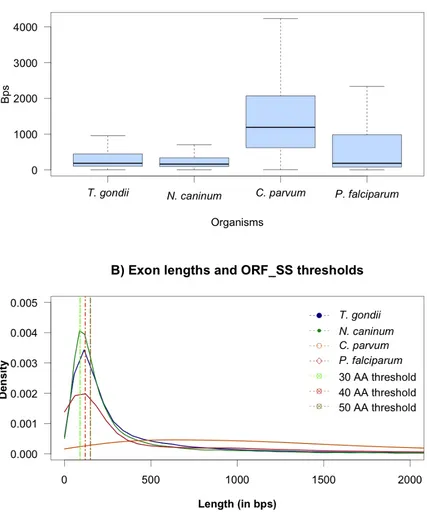
The study aimed to provide information about short coding sequences located in short open reading frames that could potentially be filtered out during ORF_SS database generation. Figure 2:2 presents a boxplot and density plot of the exon lengths across the genome of all four parasites. The median of the boxplot shows the central tendency, which is 186, 162 and 186 bps for T. gondii, N. caninum and
median value of 1191 bps and a lower interquartile of 621 bps. For the other three species the lower interquartile is 104, 96 and 81 bps respectively. The higher interquartile shows similarities between T. gondii and N. caninum (446 and 339 bps respectively) and similarities between P. falciparum and C. parvum
(983 and 2070 bps). This is related to the number of exon per gene (Figure 2:1). The whiskers are drawn to indicate the minimum and maximum values that for
Figure 2:2 A) The boxplot shows the exon distribution and the extreme values (whiskers) across apicomplexan parasites from C. parvum 4.3, P. falciparum 5.5, N. caninum 5.1 and T.
gondii 5.1. As C. parvum 4.3 and P. falciparum 5.5 have mainly single or double exon genes
within 2000 bps limit. B) The density plot shows the length densities of the exons and from the data it is clear how T. gondii and N. caninum 5.1 could benefit from precise threshold length for ORF_SS. The ORF_SS thresholds of 30 and 40 amino acids have been displayed here. The different density of lengths can help chose appropriate filter for ORF_SS prediction.
For instance in Figure 2:2 it is possible to note the median length among all exons as well as their interquartile and extreme values of the two species. Although both genomes show a similarity in gene structure (number of exon per gene), the total number of genes between these two species appears to be significantly different. The annotation of Neospora caninum 5.1, with 5587 predicted genes, appears to have 2406 genes less than in the Toxoplasma gondii (ME49) annotation. These similarities and differences allowed us to make use of known structures from well-curated genomes to aid the gene curation for the newly sequenced organism Neospora caninum.
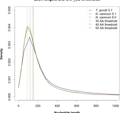
Figure 2:3 The release 6.0 of N. caninum shows an increase in similarity towards the T. gondii structure with a smaller density of exons 100-120 bps long.
2.4.2 Defining the optimum length of ORF_SS
a different start. This information was used to decide the most appropriate threshold for the minimum length of ORF_SS from a six-frame translation.
The main objective was to keep the threshold as low as possible to include as many potentially valid sequences to be contained in the database, including atypically short ones, while maintaining statistical power in the results of the search. From the data gathered for N. caninum release 5.1 about ~27% of all 40,570 exons were sequences below 33 amino acids and about ~31% have length comprised between 30 and 66 amino acids (Figure 2:3).
Our databases were generated using four values as threshold: one with no threshold (to include every sequence comprised between two stop codons) and the other three having respectively 30, 40 and 50 amino acids as the minimum length. The database size was 218Mb for threshold set at zero, and for the others was respectively 140Mb, 121Mb and 105Mb (Table 2:1).
[image:63.595.85.395.395.620.2]2.4.3 Datasets comparisons
The results from the first tests helped to formulate the best threshold level for a reasonable trade-off between database size and true positive - false positives ratio (Figure 2:5). It appears that all ORF_SS sequence databases returned very similar results (in this case the score is represented by the total number of TP PSMs at a fixed FDR threshold). In order to test the differences in ORF_SS threshold and evaluate how it affects identification of PSMs and peptide sequences it was decided to combine 10 slices from the same 1DE gel for N. caninum 5.1 (Figure 2:5). Merging all results into one dataset could potentially alter the statistical scoring of the final dataset. However querying each slice individually could increase the completeness for protein identification as these slices were sourced from different mass spectrometry runs.
Next all the individual results for each database search were re-scored individually by FDR with a maximum threshold of 5%; in the following step all of these were combined into one file per search database where the sequence redundancy had been replaced by a counter of PSMs based on the peptide sequence alone. The final output provided all TP non-redundant peptide sequences found in each database, excluding all false positives, listing the lowest FDR found in case the peptide had been matched multiple times. An internally designed pipeline algorithm was used to perform a post-processing comparison of all sequences on both outputs mutually inclusive and exclusive sets of peptides (see Figure 2:4 for workflow). The final lists highlight whether specific peptide sequences are unique to either the ORF_SS database or to gene model databases, or common to both.
Figure 2:4 The workflow for the post-processing algorithm. Tandem MS data are queried with database search engine (DB SE) against different databases. The results are then individually rescored by fixed FDR and the redundancy is removed at peptide level. Finally the results from each datasets are compared organising them into mutually exclusive/inclusive sets of peptides.
The next comparison was the ORF_SS_40 sequence database versus the current available gene model (N. caninum 5.1); to provide an insight on the current state of the annotation, as ideally, querying optimal gene models should produce significantly higher number of high confidence PSMs. Table 2:2 shows this comparison and it is clear that the official genome annotation (OGM) has been significantly outperformed by searches against the ORF_SS database, indicating that the current annotation could be improved; it was decided to repeat this comparison on other two organisms Toxoplasma gondii and Cryptosporidium parvum for which the genome annotation, to our knowledge, had higher quality.
Table 2:2 The counts of true positive PSMs and the peptide sequences at 1% FDR from 10 slices from the same 1DE gel for N. caninum. The results from ORF_SS database score, at PSM level, ~36% better than the official annotation from the same release; at peptide level there is a ~7% gain. The alternative gene model offers similar outcomes (~18% and ~12% gain for PSM and peptide level respectively), indicating that improvements in the gene models are still possible.
structure of the genome itself as 95% of the genes are single exon genes. The results from querying the official gene model (4.1 release) and the ORF_SS 40 database differ by ~3% for PSMs identification and ~3.6% for non-redundant peptides – with slightly improved performance seen for ORF_SS, potentially indicating some genes have been missed in this annotation.
![Figure 1:14 The FDR and PEP scoring curves drawn in the study by Käll et all [145] visualise](https://thumb-us.123doks.com/thumbv2/123dok_us/8062430.226202/38.595.136.470.243.506/figure-fdr-scoring-curves-drawn-study-kall-visualise.webp)