Two Dimensional CFD Simulation of Reducing Operating Pressure Effect on the System Hydrodynamics in a Downer Reactor

Article

Two-Dimensional CFD Simulation of Reducing

Operating Pressure Effect on the System

Hydrodynamics in a Downer Reactor

Pilaiwan Chaiwang1_{, Benjapon Chalermsinsuwan}1,2_{, and Pornpote Piumsomboon}1,2,_*

1 Fuels Research Center, Department of Chemical Technology, Faculty of Science, Chulalongkorn University, 254 Phayathai Road, Pathumwan, Bangkok 10330, Thailand

2 Center of Excellence on Petrochemical and Materials Technology, Chulalongkorn University, 254 Phayathai Road, Pathumwan, Bangkok 10330, Thailand

*E-mail: [email protected]

Abstract. The effect of the system hydrodynamics in a circulating fluidized bed downer (CFBD) reactor with a reducing operating pressure and solid mass flux on the hydrodynamics in a downer reactor were evaluated using a two-dimensional computational fluid dynamics simulation. Five low operating pressure conditions (0.90 to 0.99 atm) and four different solid mass fluxes (250 to 1,000 kg/m2 _{s) were explored. The simulation}

results demonstrated that the CFBD reactor had a higher mean free path when operated with a low solid mass flux than with a high solid mass flux. Moreover, a large difference between the operating and atmospheric pressures induced a high system turbulence or oscillation. The CFBD reactor with hydrodynamic fluctuation showed a good solid circulation between the gas and solid particles, as reflected by the solid volume fraction and velocities and granular temperature. These phenomena will be suitable for the chemical reaction systems. Therefore, a suitable solid mass flux was in the range of 500 to 750 kg/m2 _{s for all operating pressures under study because of the appropriate solid}

particle amount and the mixing in the system.

Keywords: Computational fluid dynamics, circulating fluidized bed downer reactor, hydrodynamics, reduced pressure, simulation.

ENGINEERING JOURNAL Volume 21 Issue 2 Received 16 May 2016

1.

Introduction

The circulating fluidized bed (CFB) system has been successfully used in both academic studies and industrial processes for the past several decades because it improves the contact between gas and solid particles, reduces gas bubbles and provides high heat and mass transfers between the phases [1]. Conventionally, this system consists of two main sections: a riser section, which carries solid particles up against the gravity force, and a downer section where the solid particles move downwards by gravity in the downer section. Due to lower energy requirement for flowing gas and solid particles, the downer section (reactor) is gaining more attention [2]. The lateral profiles of micro- and macro- flows in the downer reactor are more uniformly distributed than the ones in the riser reactor [3-6]. Therefore, it is desirable to better understand the downer reactor for applying in many novel applications. In the downer reactor, the gas and solid particle flow co-currently downward in the same direction of gravitational force. The dispersed solid particles in the axial and radial directions caused a mixing inside the system [7]. Recently, computational fluid dynamics (CFD), which is a numerical algorithm, was widely used for solving complicated equations and analyzing data, for example, heat transfer, fluid flow and chemical reactions. CFD simulation is appropriate for multiphase flow, such as fluidization. Two- and three- dimensional downer reactors were explored in many literatures using the Eulerian-Eulerian approach [8-11]. The calculation of cluster sizes in the simulation compared well with the experimental data in the lateral profile [12, 13].

In recent years, global warming has become an important issue that needs to be solved urgently. The increasing global temperature changes the global and local environmental and ecological balance. One of the main reasons for the climate change phenomena is the increasing levels of carbon dioxide (CO2)

emission. Many researchers have tried to invent various processes for capturing CO2 from flue gas, such as

membrane diffusion, solvent absorption, molecular sieves and cryogenic fractionation. However, these processes are high energy-consuming and expensive [14]. Therefore, a major research challenge is to find suitable methodologies for capturing CO2 that is economically, environmentally and technically possible

and sustainable. Dry alkali metal-based solid sorbents (K2CO3 and Na2CO3) are one innovative method that

has gained more attention due to their low energy-consumption and cost-effective nature [15-17]. However, a better understanding of this and the design of the downer reactor with an optional addition of reducing pressure is then an important requirement.

In this study, the system hydrodynamics of the downer reactor in a CFB downer (CFBD) reactor with a reduced operating pressure attained by vacuum vent was investigated by computational fluid dynamics (CFD) simulation. The basis of using the current system is for desorbing CO2 using dry solid sorbent

capture process. Several solid mass fluxes were used to compare the flow behavior in axial and radial directions. The solid volume fraction and velocity distributions of the solid particles, as well as the granular temperature, were illustrated and discussed with five different reducing pressures and four different solid mass fluxes.

2.

Computational Fluid Dynamics (CFD) Simulation Model

2.1. System Description, Computational Domain, Boundary and Operating Conditions

In this study, the CFD simulations were conducted in the downer reactor of a cold flow two-dimensional CFB system. A simplified schematic representation of the CFBD reactor with a total height of 0.60 m and a width of 0.20 m and 0.10 m diameter at the expanded (De) and contracted (Dc) zones, respectively, is

shown in Fig. 1(a), whilst the computational domain of the simplified CFBD reactor is illustrated in Fig. 1(b).

The gas and solid particles entered the system from the top of the downer reactor with a certain velocity at atmospheric pressure. Nitrogen gas (N2) was fed from the two-sided inlets at a slope angle above

the bottom of the downer reactor at a two-fold higher velocity than the minimum fluidization velocity (2Umf). The vacuum vents were connected through two symmetrical side outlets, 0.30 m below the top of

the downer reactor. The solid mass that entered the downer reactor was evaluated at 250, 500, 750 and 1,000 kg/m2 _{s. The other simulation boundary and operating conditions are listed in Table 1. Initially, there}

(particle), restitution coefficient (wall) and specularity coefficient were selected from the literature with similar CFBD system.

(a) (b)

Fig. 1. (a) Schematic drawing and (b) computational domains and their boundary conditions of the simplified CFBD reactor used in this study. De and Dc represent the expanded and contracted zones, respectively.

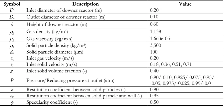
Table 1. Parameters used in this study.

Symbol Description Value

Di Inlet diameter of downer reactor (m) 0.20 Do Outlet diameter of downer reactor (m) 0.10 h Height of downer reactor (m) 0.60

g Gas density (kg/m3) 1.138

g Gas viscosity (kg/ms) 1.663e-05

s Solid particle density (kg/m3) 3,500

dp Solid particle diameter (µm) 100

vg Inlet gas velocity (m/s) 0.20

vs Inlet solid velocity (m/s) 0.18, 0.36, 0.51, 0.71

s Inlet solid volume fraction (-) 0.40

P Pressure/Reducing pressure at outlet (atm) 0.90/-0.10, 0.925/-0.075, 0.95/ _{-0.05, 0.975/-0.025, 0.99/-0.01}

e Restitution coefficient between solid particles (-) 0.90

ew Restitution coefficient between solid particle and wall (-) 0.95

2.2. Mathematical Model

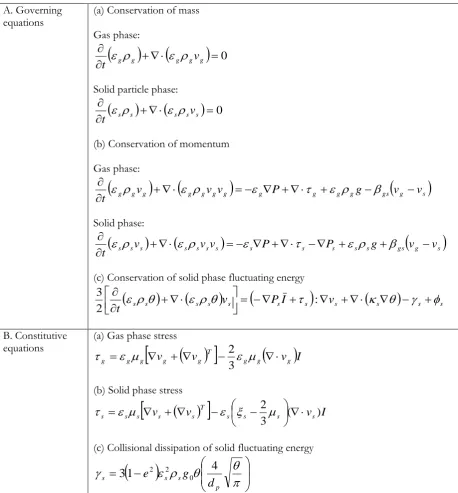
In this cold flow CFD simulation, the mass and momentum conservation equations were solved using numerical algorithms. The methodology for computing the gas-solid particle flow patterns can be broadly divided into Eulerian-Eulerian (E-E) and Eulerian-Lagrangian (E-L) based groups. Most fluidization studies have used the E-E model as the appropriate system [22, 23] and the Gidaspow model for the selected drag force or interphase exchange coefficient. This drag force is claimed to match the dense fluidization system and is similar to this study system [24]. To close the governing equations and completely explain the solid particle characteristics, the kinetic theory of granular flow was employed [25]. The modeling was carried out using Ansys Fluent 6.2.16, a commercial CFD software. To couple the pressure and velocity, this study was used phase coupled SIMPLE algorithm. A summary of all the conservation and constitutive equations is given in Table 2.

Table 2. A summary of the governing and constitutive equations.

A. Governing

equations (a) Conservation of mass Gas phase:









  g g g g g v

t









Solid particle phase:









  s s s s s v

t









(b) Conservation of momentum

Gas phase:













t       





_

_

_

_

_

_

_

_

_

Solid phase:













t        





_

_

_

_

_

_

_

_

_

(c) Conservation of solid phase fluctuating energy

















t























   _   : 2 3 B. Constitutive

equations (a) Gas phase stress



_{ }



_

_

v g g g

T g g

g g

g 











3 2

(b) Solid phase stress









T s s

s s

s ( )

3

2 _{ }

     _     













(c) Collisional dissipation of solid fluctuating energy





_































d

g

e

4

1

(d) Radial distribution function 1 3 / 1 max , 0

1





































g





(e) Solid phase pressure



g

(

e

)



P









1



2



1



(f) Solid phase shear viscosity

2

0 0

0

(

1

)

5

4

1

)

1

(

96

10

)

1

(

5

4









_

_









g

e

g

e

d

e

g

d

s



















(g) Solid phase bulk viscosity











(

1

)

3

4

e

g

d

s





(h) Exchange of the fluctuating energy between gas and solid particle











3

(i) Gas–solid phase interphase exchange coefficient

Gidaspow model: when

;

80

.

0













d

v

v

d























150

1

1

.

75

1

2 when

;

80

.

0









0

1

4

3

gs

v

v

C

d

















;

1000

Re







0 1 015

24 .

D . Re

Re

C  

g p s g g

g

v

v

d

Re











;

1000

Re



C



0

.

44

3.

Results and Discussion

3.1. Validation of the CFD Model

3.1.1. Grid independence test

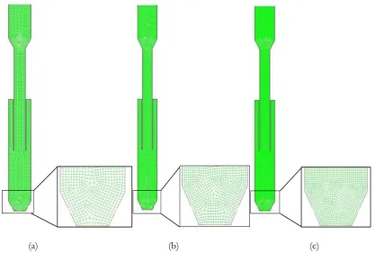
significant deviations in the obtained results when using the 4,000 mesh compared to computational cells with 8,000 or 12,000 meshes because of the large gradients in the properties of the flow. However, the results obtained with computational cells of 8,000 and 12,000 meshes were quite similar. Hence, accruing more computational cells than 8,000 meshes did not significantly affect the prediction, and so computational cells with 8,000 meshes were applied for the calculation in the following sections.

(a) (b) (c)

Fig. 2. Grid independency test with computational cells of (a) 4,000, (b) 8,000 and (c) 12,000 meshes.

3.1.2. Quasi-steady state test

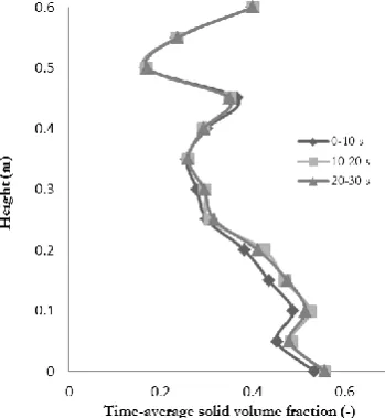
In order to systematically explain the results, the quasi-steady state time-averaged range requires clarification, and so the results were averaged after the system reached a quasi-steady state condition. Comparison of the computed time-averaged solid volume fraction profiles for the CFBD reactor with three different time-averaged ranges (Fig. 4) revealed similar solid volume fraction results with 10–20 s and 20–30 s time-averaged ranges, but that from the shorter 0–10 s time-averaged range was slightly different. Thus, the CFBD reactor had entered the quasi steady-state conditions from simulation times of more than 10 s, and so in this study the CFD model used the 10–30 s time-averaged range of the simulation time.

Fig. 4. The computed solid volume fraction profiles in the CFBD reactor when derived from different time-averaged ranges.

3.2. Comparison of the System Hydrodynamics

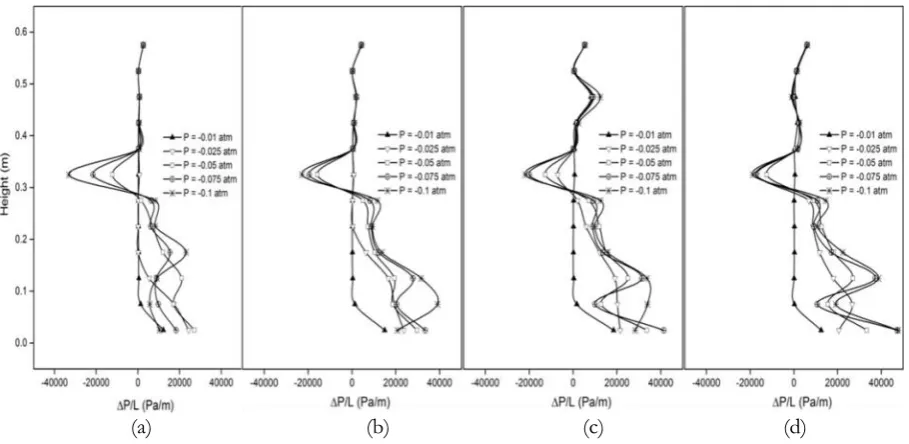
3.2.1. Axial pressure profile

The axial pressure and pressure drop profiles in the CFBD reactor with five different reducing pressures (-0.01 to -0.10 atm) and four solid mass fluxes (250, 500, 750 and 1,000 kg/m2 _{s) are shown in Figs. 5 and 6,}

respectively. The pressure drop in this study can be defined from the absolute pressure in the axial profile along the downer system per unit length. Thirteen cross-sectional areas were measured through the corresponding section length in axial levels of 0.0, 0.05, 0.10, 0.15, 0.20, 0.25, 0.30, 0.35, 0.40, 0.45, 0.50, 0.55 and 0.60 m. The obtained time- and area- averaged absolute pressure per unit length were used to calculate pressure drop profiles. The axial pressure distributions are decreased along the CFBD reactor when reducing the operating pressures. When the solid mass flux increased, the absolute pressure near the bottom section increased. Moreover, it can be seen that the pressure drop profiles for all the solid mass fluxes were close to zero and gravitated uniformly until 0.40 m system height above the bottom region. Below 0.40 m system height above the bottom region, the simulation results showed that the pressure drop was significantly fluctuated due to the connecting position of outlet vacuum vent that disturbed and lowered the pressure drop inside the system. Below the outlet vacuum vent, the pressure drop again drastically oscillated to match with the pressure at bottom outlet. At the bottom section, the distributions of the pressure drop profiles had shown positive values since the solid particles were accelerated by gravity more than the drag force in the upward direction. The pressure drop across the fluidized bed can be employed to calculate the net weight of the solid particles. Comparing the different operating pressures, operating pressures of 0.90 and 0.99 atm gave the highest and lowest deviation in the pressure drop profiles, respectively. In addition, the reducing pressures of -0.01 and -0.025 atm had the lowest pressure drop fluctuation at the solid mass flux of 250 kg/m2_{s and increased with the solid mass flux while the reducing}

pressure of -0.1 atm had the highest pressure drop fluctuation at the solid mass flux of 250 kg/m2_{s and}

atm were constant throughout the simulation. This can be explained by the amount of solid particle inside the system and the available movable space.

(a) (b) (c) (d)

Fig. 5. The computed time-averaged pressure profiles in the CFBD reactor with a solid mass flux of (a) 250, (b) 500, (c) 750 and (d) 1,000 kg/m2 _{s at five different reducing pressures.}

(a) (b) (c) (d)

Fig. 6. The computed time-averaged pressure drop profiles in the CFBD reactor with a solid mass flux of (a) 250, (b) 500, (c) 750 and (d) 1,000 kg/m2 _{s at five different reducing pressures.}

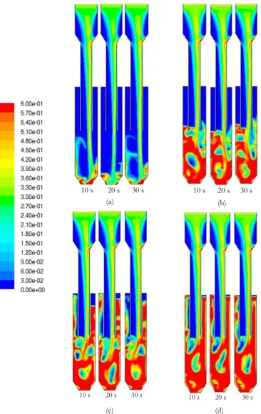
3.2.2. Solid volume fraction

The instantaneous contours of the solid volume fraction at an outlet pressure of 0.95 atm with solid mass fluxes of 250, 500, 750 and 1,000 kg/m2_{s are shown in Fig. 7, where the observed flow behaviors at a}

bubbles then occurred inside the system especially at the centre region. These fluctuations increased with an increasing solid mass flux as a result of the high circulation between gas and solid particles. There is a lot of empty space in the CFBD reactor with the low (250 kg/m2_{s) solid mass flux, but this decreased to almost}

half of the expanded zone (De) at the higher solid mass flux of 500 kg/m2s. The solid volume fraction

could be separated into the two main regions of the dilute and dense regions at the top and bottom of the CFBD reactor, respectively [26]. On the other hand, there was no apparent empty space in the CFBD reactor at the higher solid mass flux of 750 and 1000 kg/m2_{s, and the system could not be visibly separated}

into different regions. Rather, the increased solid mass flux resulted in the solid particles just moving up to reach the vacuum vent at 0.30 m below the top of the CFBD reactor. Thus, this downer height is likely to be insufficient for a solid mass flux greater than 750 kg/m2_{s as the solid particles were flown out of the}

system.

The time- and area- averaged solid volume fraction profiles in the CFBD reactor with the five different reducing pressures and four solid mass fluxes are depicted in Fig. 8. At the inlet, the solid particles were input to the CFBD reactor across the whole cross-sectional area with an initial solid volume fraction of 0.40. As the solid particles flew into the contracted zone (Dc), the solid volume fraction decreased to 0.20–0.30,

and then the solid particles accumulated again at the bottom section. Decreasing the operating pressure slightly affected the solid volume fraction at about 0.30 m below the entrance, with a lot of change between the exit and about 0.30 m above the outlet of the CFBD reactor among the different operating pressures. At the highest outlet pressure (0.99 atm), the lowest solid volume fraction was found for all solid mass fluxes, which could be explained as that it has the lowest difference between the operating pressures. Decreasing the operating pressure resulted in the solid particles being more expanded in the CFBD reactor, consistent with that previously reported [27], except at the lowest solid mass flux (250 kg/m2_{s) where the}

trend was not clearly seen due to the low density (quantity) of solid particles.

The available space in the CFBD reactor is inversely proportional to the solid mass flux, since the solid particles are able to move freely in the vacant places. Thus, the mobility of the solid particles infers the turbulence inside the system. The solid particles accumulated near the bottom outlet at all operating pressures except for that at the highest pressure (0.99 atm). The observed fluctuations with different operating pressures showed no clear trend with the radial solid volume fraction, which is similar to that previously reported in the conventional system hydrodynamics in a riser reactor with a bubbling fluidized bed regime but is different to that reported in a CFBD [5, 28]. The gas bubbles that occur inside the system are likely to make the system highly heterogeneous.

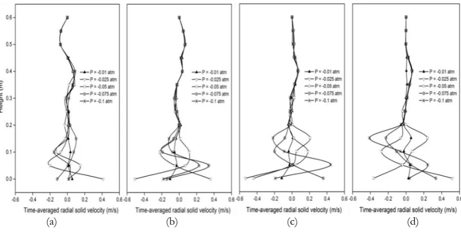
3.2.3. Radial solid particle velocities

The time- and area- averaged radial solid particle velocity profiles in the CFBD reactor with the five different reducing pressures and four different solid mass fluxes revealed a uniform distribution while entering the entrance, but oscillated at a height approximately 0.20 m above the bottom outlet (Fig. 9). The distributions of the radial solid particle velocities had both positive and negative values, which imply that the solid particle motions were randomly moving to the left and right system sides. As the solid mass flux and reducing pressure inside the system increased then so the radial solid particle velocities oscillated more.

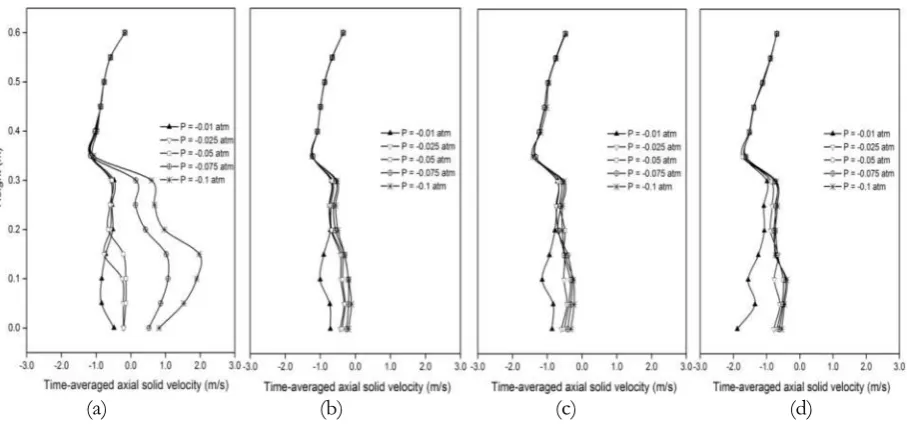
3.2.4. Axial solid particle velocities

The time- and area- averaged axial solid particle velocity profiles in the CFBD reactor at the five different reducing pressures and four solid mass fluxes are illustrated in Fig. 10. The solid particles entered the system with a period of free-fall condition from the top of the downer, the axial solid particle velocity profiles were initially close to zero. The negative values above the bottom outlet of the CFBD reactor roughly at 0.35 m were resulted from the solid particle motions moving downward. Then, particle velocity increased and remained constant near the outlet section since the drag force had increased to equal the gravitational force. Increasing the amount of solid particles and operating pressure did not significantly affect the axial solid velocity profiles, which remained evenly distributed along the height of the CFBD reactor except for with a solid mass flux of 250 kg/m2 _{s. Under that low solid mass flux condition, the axial}

Fig. 7. The instantaneous contours of the solid volume fraction with solid mass fluxes of (a) 250, (b) 500, (c) 750 and (d) 1,000 kg/m2 _{s at an operating pressure of 0.95 atm.}

20 s 30 s

10 s 10 s 20 s 30 s

20 s 30 s 10 s

(a) _(b)

(c)

20 s 30 s 10 s

(a) (b) (c) (d)

Fig. 8. The computed time-averaged solid volume fraction profiles in the CFBD reactor with a solid mass flux of (a) 250, (b) 500, (c) 750 and (d) 1,000 kg/m2 _{s at five different reducing pressures.}

(a) (b) (c) (d)

(a) (b) (c) (d)

Fig. 10. The computed time-averaged axial solid particle velocity profiles in the CFBD reactor with a solid mass flux of (a) 250, (b) 500, (c) 750 and (d) 1,000 kg/m2 _{s at five different reducing pressures.}

3.2.5. Granular temperature

The granular temperature is the kinetic energy of an oscillating solid particle. The definition of granular temperature can be described as the random kinetic energy of the random motion of the particles. Chalermsinsuwan et al. [5, 28], Tartan [29] and Tartan and Gidaspow [30] defined the equations for calculating granular temperature as shown in Eq. (1):

' ' '

' '

'

3

1

3

1

3

1

)

,

(

t

x



v

v



v

v



v

v



The variances of fluctuating velocity in the direction of the axial flow are approximately 2 to 3 times higher than those in the radial and tangential directions. In developed flow, the radial, and tangential velocities are quite small and, hence, their gradients are also small. For the CFD modeling in a two-dimensional system, the velocity in the radial direction or non-flow direction is assumed to be the same. The turbulent granular temperature then can be calculated using Eq. (2):

' ' '

'

3

1

3

2

)

,

(

t

x



v

v



v

v



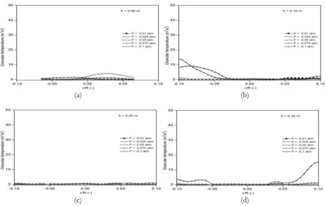
A high granular temperature reflects particles with a high energy that can make them move or shake. Thus, solid particles with a high granular temperature can move more independently than those with a low granular temperature. The time- and area- averaged granular temperature in the CFBD reactor with the five different reducing pressures and four solid mass fluxes (Fig. 11) revealed that the granular temperature significantly affected the system at a solid mass flux of less than 1000 kg/m2 _{s. This is because there were}

low solid particles in the system at those solid particle flow rates. The highest operating pressure (0.99 atm) resulted in a high granular temperature at the top section, whereas at the lower operating pressure of 0.90 atm there was a high granular temperature at the center and the bottom sections. As the solid mass flux increased, the oscillations in the dense system were lower than those in the dilute system because of the available space between solid particles or solid particle clusters. The radial distributions of the time-averaged granular temperature in the CFBD reactor also revealed that the highest granular temperature at all heights above the bottom outlet was found at the lowest operating pressure (0.90 atm), with that for the representative solid mass fluxes of 500 and 750 kg/m2 _{s are shown in Figs. 12 and 13, respectively.}

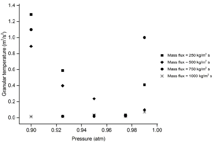
To present the results more generally and specifically for the downer reactor system, the comparison of the averaged total granular temperatures at four different mass fluxes with five reducing pressures is displayed in Fig. 14. For the system with solid mass flux less than 1,000 kg/m2 _{s, the reducing pressure had}

available movable space. The fluctuation inside the system was lowest for the reducing pressure of -0.025 atm. On the other hand, the total granular temperature at solid mass flux of 1,000 kg/m2 _{s was low}

independently from pressure reduction because of the high amount of solid particle inside the system.

(a) (b) (c) (d)

Fig. 11. The computed time-averaged granular temperature profiles in the CFBD reactor with a solid mass flux of (a) 250, (b) 500, (c) 750 and (d) 1,000 kg/m2 _{s at five different reducing pressures.}

(a) (b)

(c) (d)

Fig. 12. The radial distributions of the time-averaged granular temperature at a CFBD reactor height (h) of (a) 0.00, (b) 0.10, (c) 0.20 and (d) 0.30 m with a solid mass flux of 500 kg/m2 _{s at five different reducing}

(a) (b)

(c) (d)

Fig. 13. The radial distributions of the time-averaged granular temperature at a CFBD reactor height (h) of (a) 0.00, (b) 0.10, (c) 0.20and (d) 0.30m with a solid mass flux of 750kg/m2 _{s at five different reducing}

pressures.

4.

Conclusion

The CFD-based hydrodynamics simulation was evaluated in a CFBD reactor with five reduced operating pressures (0.90–0.99 atm) and four different solid mass fluxes (250–1000 kg/m2 _{s) using a two-dimensional}

CFD simulation. The simulation results demonstrated that the CFBD reactor with a low solid mass flux (250 kg/m2 _{s) had a greater ability of the solid particles to move than when at a high solid mass flux}

operating condition. With respect to the effect of the reduced operating pressure, the large difference between the operating pressure and atmospheric pressure gave a high system turbulence or oscillation, and accordingly a good solid circulation between gas and solid particles, as seen from the solid volume fraction, solid particle velocities and granular temperature. In this study, the suitable mass flux was found to be between 500 to 750 kg/m2 _{s in terms of providing the appropriate solid particle amount and mixing in the}

system. However, this is only a preliminary study for the CFBD reactor under a reduced operating pressure. Therefore, further studies should be performed to find the feasibility and appropriateness of the CFBD reactor under a reduced operating pressure.

Acknowledgements

The authors gratefully acknowledge the financial support for this study from the Thailand Research Fund (TRF) through the Royal Golden Jubilee Ph.D. Program, Fuels Research Center, Chulalongkorn University (Grant No. PHD/0356/2551), and the Center of Excellence on Petrochemical and Materials Technology, Chulalongkorn University.

Notations

General letters

C

Drag coefficient (-)

d

Diameter of catalyst/solid particle (m)

D

Diameter at contracted zone (m)

D

Diameter at expanded zone (m)

D

Inlet diameter of downer reactor (m)

D

Outlet diameter of downer reactor (m)

e

Restitution coefficient between solid particles (-)

e

Restitution coefficient between solid particle and wall (-)

g

Gravitational acceleration (m/s

₎

g

Radial distribution function (-)

h

Height of downer reactor (m)

I

Unit tensor (-)

P

Gas pressure (Pa)

P

Solid particle pressure (Pa)

Re

Reynolds number (-)

t

Time (s)

U

Minimum fluidization velocity (m/s)

v

Velocity (m/s)

v’

Velocity fluctuation (m/s)

Greek letters



Gas-solid particle interphase exchange or drag coefficient (kg/s m

₎



Volume fraction (-)



Solid volume fraction at maximum packing (-)



Specularity coefficient (-)



Exchange of the fluctuating energy between gas and solid (kg/m s

₎



Conductivity of the solid fluctuating energy (kg/m s)



Viscosity (kg/m s)



Granular temperature (m

_/s

₎



Density (kg/m

₎



Stress tensor (Pa)



Bulk viscosity (kg/m s)

Subscripts

i

Direction

g

Gas phase

s

Solid particle phase

References

[1] D. Kunii and O. Levenspiel, Fluidization engineering: Elsevier, 2013.

[2] Y. Cheng, C. Wu, J. Zhu, F. Wei, and Y. Jin, “Downer reactor: from fundamental study to industrial application,” Powder Technology, vol. 183, pp. 364-384, 2008.

[3] H. Zhang, W. X. Huang, and J. X. Zhu, “Gas‐solids flow behavior: CFB riser vs. downer,” AIChE Journal, vol. 47, pp. 2000-2011, 2001.

[4] M. Zhang, Z. Qian, H. Yu, and F. Wei, “The solid flow structure in a circulating fluidized bed riser/downer of 0.42-m diameter,” Powder Technology, vol. 129, pp. 46-52, 2003.

[5] B. Chalermsinsuwan, T. Chanchuey, W. Buakhao, D. Gidaspow, and P. Piumsomboon, “Computational fluid dynamics of circulating fluidized bed downer: Study of modeling parameters and system hydrodynamic characteristics,” Chemical engineering Journal,vol. 189, pp. 314-335, 2012.

[6] Y. Prajongkan, P. Piumsomboon, and B. Chalermsinsuwan, “Computation of mass transfer coefficient and Sherwood number in circulating fluidized bed downer using computational fluid dynamics simulation,” Chemical Engineering and Processing: Process Intensification, vol. 59, pp. 22-35, 2012. [7] F. Wei and J.-X. Zhu, “Effect of flow direction on axial solid dispersion in gas—Solids cocurrent

upflow and downflow systems,” The Chemical Engineering Journal and the Biochemical Engineering Journal, vol. 64, pp. 345-352, 1996.

[8] K. Ropelato, H. F. Meier, and M. A. Cremasco, “CFD study of gas–solid behavior in downer reactors: an Eulerian–Eulerian approach,” Powder Technology, vol. 154, pp. 179-184, 2005.

[9] T. Samruamphianskun, P. Piumsomboon, and B. Chalermsinsuwan, “Computation of system turbulences and dispersion coefficients in circulating fluidized bed downer using CFD simulation,”

Chemical Engineering Research and Design, vol. 90, pp. 2164-2178, 2012.

[10] X. Lan, W. Yan, C. Xu, J. Gao, and Z.-H. Luo, “Hydrodynamics of gas–solid turbulent fluidized bed of polydisperse binary particles,” Powder Technology, vol. 262, pp. 106-123, 2014.

[11] G.-Q. Chen and Z.-H. Luo, “New insights into intraparticle transfer, particle kinetics, and gas–solid two-phase flow in polydisperse fluid catalytic cracking riser reactors under reaction conditions using multi-scale modeling,” Chemical Engineering Science, vol. 109, pp. 38-52, 2014.

[12] Y. Cheng, Y. Guo, F. Wei, Y. Jin, and W. Lin, “Modeling the hydrodynamics of downer reactors based on kinetic theory,” Chemical Engineering Science, vol. 54, pp. 2019-2027, 1999.

[13] S. Li, W. Lin, and J. Yao, “Modeling of the hydrodynamics of the fully developed region in a downer reactor,” Powder technology, vol. 145, pp. 73-81, 2004.

[14] D. Nikomborirak, “Gas in Thailand,” in The Impacts and Benefits of Structural Reforms in Transport, Energy and Telecommunications Sectors. APEC Policy Support Unit, Singapore,2011, pp. 385-397.

[15] C.-K. Yi, S.-H. Jo, Y. Seo, J.-B. Lee, and C.-K. Ryu, “Continuous operation of the potassium-based dry sorbent CO 2 capture process with two fluidized-bed reactors,” International Journal of Greenhouse Gas Control, vol. 1, pp. 31-36, 2007.

[16] C.-K. Yi, S. Jo, Y. Seo, S. Park, K. Moon, J. Yoo, J. B. Lee, and C. K. Ryu, “CO2 capture

[17] L. Li, Y. Li, X. Wen, F. Wang, N. Zhao, F. Xiao, W. Wei, and Y. Sun, “CO2 capture over

K2CO3/MgO/Al2O3 dry sorbent in a fluidized bed,” Energy and Fuels, vol. 25, p. 3835, 2011.

[18] S. C. Lee, B. Y. Choi, T. J. Lee, C. K. Ryu, Y. S. Ahn, and J. C. Kim, “CO2 absorption and

regeneration of alkali metal-based solid sorbents,” Catalysis Today, vol. 111, pp. 385-390, 2006.

[19] S. C. Lee, Y. M. Kwon, C. Y. Ryu, H. J. Chae, D. Ragupathy, S. Y. Jung, J. B. Lee, C. K. Ryu, and J. C. Kim, “Development of new alumina-modified sorbents for CO2 sorption and regeneration at

temperatures below 200ºC,” Fuel, vol. 90, pp. 1465-1470, 2011.

[20] Y. C. Park, S.-H. Jo, K.-W. Park, Y. S. Park, and C.-K. Yi, “Effect of bed height on the carbon dioxide capture by carbonation/regeneration cyclic operations using dry potassium-based sorbents,” Korean Journal of Chemical Engineering, vol. 26, pp. 874-878, 2009.

[21] P. C. Johnson and R. Jackson, “Frictional–collisional constitutive relations for granular materials, with application to plane shearing,” Journal of Fluid Mechanics, vol. 176, pp. 67-93, 1987.

[22] M. Van der Hoef, M. van Sint Annaland, N. Deen, and J. Kuipers, “Numerical simulation of dense gas-solid fluidized beds: A multiscale modeling strategy,” Annu. Rev. Fluid Mech., vol. 40, pp. 47-70, 2008.

[23] B. Chalermsinsuwan, P. Kuchonthara, and P. Piumsomboon, “CFD modeling of tapered circulating fluidized bed reactor risers: hydrodynamic descriptions and chemical reaction responses,” Chemical Engineering and Processing: Process Intensification, vol. 49, pp. 1144-1160, 2010.

[24] A. Fluent, 14.0 User’s Manual. Canonsburg, PA: ANSYS Inc.,2011.

[25] D. Gidaspow, Multiphase Flow and Fluidization: Continuum and Kinetic Theory Descriptions. Academic press, 1994.

[26] S. Kongkitisupchai and D. Gidaspow, “Carbon dioxide capture using solid sorbents in a fluidized bed with reduced pressure regeneration in a downer,” AIChE Journal, vol. 59, pp. 4519-4537, 2013.

[27] H. Chen and H. Li, “Characterization of a high-density downer reactor,” Powder Technology, vol. 146, pp. 84-92, 2004.

[28] B. Chalermsinsuwan, D. Gidaspow, and P. Piumsomboon, “Two-and three-dimensional CFD modeling of Geldart A particles in a thin bubbling fluidized bed: Comparison of turbulence and dispersion coefficients,” Chemical Engineering Journal, vol. 171, pp. 301-313, 2011.

[29] M. Tartan, Fluidization in a Riser: Granular Temperature and Stresses, 2003.