OPTIMIZATION
FABRIZIO GRANDONI†, PIOTR KRYSTA‡, STEFANO LEONARDI§, AND CARMINE VENTRE¶
Abstract. In a classic optimization problem the complete input data is assumed to be known to the algorithm. This assumption may not be true anymore in optimization problems motivated by the Internet where part of the input data is private knowledge of independentselfishagents. The goal ofalgorithmic mechanism designis to provide (in polynomial time) a solution to the optimization problem and a set of incentives for the agents such that disclosing the input data is a dominant strategy for the agents. In case of NP-hard problems, the solution computed should also be a good approximation of the optimum.
In this paper we focus on mechanism design formulti-objectiveoptimization problems. In this setting we are given a main objective function, and a set of secondary objectives which are modeled via budget constraints. Multi-objective optimization is a natural setting for mechanism design as many economical choices ask for a compromise between different, partially conflicting goals. The main contribution of this paper is showing that two of the main tools for the design of approxi-mation algorithms for multi-objective optimization problems, namely approximate Pareto sets and Lagrangian relaxation, can lead to truthful approximation schemes.
By exploiting the method of approximate Pareto sets, we devise truthful deterministic and ran-domized multi-criteria FPTASs for multi-objective optimization problems whose exact version admits a pseudo-polynomial-time algorithm, as for instance the multi-budgeted versions ofminimum span-ning tree,shortest path,maximum (perfect) matching, andmatroid intersection. Our construction also applies tomulti-dimensional knapsack and multi-unit combinatorial auctions. Our FPTASs compute a (1 +ε)-approximate solution violating each budget constraint by a factor (1 +ε).
When feasible solutions induce an independence system, i.e., when subsets of feasible solutions are feasible as well, we present a PTAS (not violating any constraint), which combines the approach above with a novel monotone way to guess the heaviest elements in the optimum solution.
Finally, we present a universally truthful Las Vegas PTAS for minimum spanning tree with a single budget constraint, where one wants to compute a minimum cost spanning tree whose length is at most a given valueL. This result is based on the Lagrangian relaxation method, in combination with our monotone guessing step and with a random perturbation step (ensuring low expected running time). This result can be derandomized in the case of integral lengths.
All the mentioned results match the best known approximation ratios, which are however ob-tained by non-truthful algorithms.
Key words.algorithmic mechanism design, truthful mechanisms, multi-objective optimization, approximation algorithms, monotone algorithms, approximate Pareto sets, Lagrangian relaxation.
AMS subject classifications. 91A99, 91B26, 91B32, 68Q25, 68W25, 68W40, 90B10
1. Introduction. A multi-objective combinatorial optimization problem is char-acterized by a setS ⊆2U of feasible solutions defined over a ground setU of m ele-ments, and a set of objective cost functionsℓi:U →Q+,i= 0, . . . , k. In this paper we
∗Partially supported by ERC Starting Grant NEWNET 279352, by DFG grant Kr 2332/1-2 within Emmy Noether program, by EPSRC grants EP/F069502/1 and EP/K01000X/1, by EU FET project MULTIPLEX 317532 and EU ERC project PAAI 259515. A preliminary version of this paper has appeared as [16].
†IDSIA, University of Lugano, Galleria 1, 6928 Manno-Lugano, Switzerland. Email: [email protected].
‡University of Liverpool, Department of Computer Science, Ashton Building, Ashton Street, Liverpool L69 3BX, U.K. Email: [email protected]
§Sapienza Universit`a di Roma, Dipartimento di Informatica e Sistemistica, Via Ariosto 25, 00185 Roma, Italy. Email:[email protected]
¶Teesside University, School of Computing, Greig Building, Borough Road, Middlesbrough TS1 3BA, U.K. Email: [email protected]
assumek=O(1). The aim is to find a solutionS∈ S optimizingℓi(S) =Pe∈Sℓi(e)
for all i, where optimizing means maximizing or minimizing, depending on the ob-jective. A typical way to deal with multiple objectives is turning all the objectives but one into budget constraints (see, e.g., [36] and references therein for related ap-proaches). More formally, let X be the set of incidence vectors corresponding to
S, and Bi ∈ Q+, i = 1, . . . , k, a set of budgets1. Let also best ∈ {max,min} and i∈ {≥,≤} fori= 1, . . . , k. We consider a problem P defined as:
best X
e∈U
ℓ0(e)xe
s.t. x∈ X (P)
X
e∈U
ℓi(e)xeiBi fori= 1, . . . , k.
We will often refer to the ℓ0(e)’s as costs, and calllengths the remainingℓi(e)’s. We
define0=≥ifbest= max, and0=≤otherwise. For a relation, we say thata≻b ifabanda6=b, and use≺for6andfor6≻.
This framework naturally models network design problems with resource con-straints. For example, in thebudgeted minimum spanning treeproblem (BMST) U is the set of edges of a graphG= (V, E),S is the set of spanning trees ofG,best= min and there is a unique budget constraint with1=≤. Hereℓ0(e) can be used to model, e.g, the cost of establishing a link on e, andℓ1(e) the delay on that edge. The bud-geted shortest path problem (BSP) is defined analogously, where spanning trees are replaced by the paths between two given nodes. Alternatively, (U,S) might define the intersection of two matroids.
In this paper we study this family of optimization problems from a game theo-retical point of view. (For basic notions on algorithmic game theory, see, e.g., [31]). We are given a set of selfish agents, where agent f controls elementf ∈ U. Thetype ℓf = (ℓ0(f), . . . , ℓ
k(f)) is considered as private knowledge of f. Agent f can lie by
declaring a type ℓ′f 6=ℓf, with the constraint ℓ
i(f)i ℓ′i(f) for i = 1, . . . , k (while
ℓ′
0(f) is arbitrary). In the BMST example above, agentf might declare a larger delay ℓ′
1(f) on f than the smallest possible ℓ1(f) in order to reduce her operational costs (whilef is not able to offer a delay smaller than ℓ1(f)). Moreover, f might declare a cost larger thanℓ0(f) to maximize her revenue, or a smaller cost to maximize her chances to be part of the solution. (For further motivations on this model of selfish agents please refer to Section 2.)
The main goal of (utilitarian) mechanism design is to forcef to declare her true type. This is achieved by defining a set of payments pf, f ∈ U. Payments, types
and the computed solution define agents’utility (see Section 2 for formal definitions). Payments should be defined such that saying the truth is a dominant strategy, i.e., each agent maximizes her utility by declaring her true type, independently of what the other agents declare. In that case the mechanism is truthful. At the same time, we wish to design mechanisms which compute (efficiently) a solution approximating the optimum in a standard sense, with respect to the declarations. The objective of
P is also calledsocial welfare in this context.
1Part of our results can be extended to the case that zero values of theℓ
i(e)’s andBi’s are also
1.1. Related Work. A classical technique to design truthful mechanisms is the Vickrey-Clarke-Groves (VCG) mechanism [10, 20, 39] which however requires to solve optimally the underlying optimization problem. For NP-hard problems one can use the approach of [7, 24]; therein, it is shown that, in order to obtain truthfulness, it is sufficient to design an approximation algorithm which is alsomonotone. Informally, an algorithm is monotone if, assuming that it computes a solution containing an element f for a given problem, then it computes a solution containing f also in the case that we replace, fori∈ {0,1, . . . , k},ℓi(f) with ¯ℓi(f)iℓi(f)2.
Efficient monotone algorithms are known only for a few special cases of the frame-work above. For example by setting best = max, i=≤ for all i ≥ 1, and using a trivial set of feasible solutionsS = 2U, one can model themulti-dimensional knapsack problem. For this problem a monotoneO(k1/B) approximation is given in [7], where
B is the smallest budget. Their result extends to multi-unit combinatorial auctions for unknown single-minded bidders (i.e., the setting in which bidders are interested in only one set of goods and can lie on both valuation and set itself). (See [3, 12, 13, 23] for results on more general types of bidders.) A monotone PTAS is known formultiple knapsack[7], which can be modeled in our framework by letting one agent control a constant number of elements. This extends tomulti-unit unit-demand auctionsfor un-known multi-minded bidders with the same valuation for each alternative. For graph problems, monotone FPTASs are known for BSP and for BMST in the special case of bounded-treewidth graphs [7]. We note that these FPTASs do not violate the budget constraint, but it is not clear how to extend them to more than one budget. An-other related result is a bicriteria monotone algorithm for the spanning arborescence problem [5].
Multi-budgeted optimization in the standard (non-game-theoretical) sense is ex-tensively studied in the literature. There are a few general tools for designing ap-proximation algorithms for budgeted problems. One basic approach is combining dynamic programming (which solves the problem for polynomial costs and lengths) withrounding and scalingtechniques (to reduce the problem to the case of polynomial quantities). This leads for example to an FPTAS for BSP [21, 25, 40].
Another fundamental technique is the Lagrangian relaxation method. The basic idea is relaxing the budget constraints, and lifting them into the objective function, where they are weighted by Lagrangian multipliers. Solving the relaxed problem, one obtains two or more solutions with optimal Lagrangian weight, which can—if needed— be patched together to get a good solution for the original problem. Demonstrating this method, Goemans and Ravi [35] gave a PTAS for BMST, which also extends to 1-budgeted matroid basis. Inspired by this approach, Correa and Levin [11] presented algorithms for special classes of polynomial-time covering problems with an additional covering constraint. Using the same approach as Goemans and Ravi, with an involved patching step, Berger, Bonifaci, Grandoni, and Sch¨afer [4] obtained a PTAS for 1-budgeted matching and 1-1-budgeted matroid intersection independent set. A PTAS for 2-budgeted matching was obtained by Grandoni and Zenklusen [18, 19]. The authors also present a PTAS for k-budgeted matroid independent set, k =O(1). Finally a PTAS for k-budgeted matching was given by Chekuri, Vondr´ak, and Zenklusen [9].
2Sometimes in the literature a weaker notion of monotonicity is considered, where only the cost
ℓ0(f) can change. Typically it is much simpler to adapt known approximation algorithms to achieve
The authors also present a PRAS fork-budgeted matroid intersection3.
The mentioned algorithms provide strictly feasible solutions. Sometimes one searches for multi-criteria PTASs, which compute a (1 +ε)-approximate solution violating the budgets by a factor (1 +ε). Papadimitriou and Yannakakis [32] de-scribe a very general technique, based on the construction of ε-approximate Pareto sets (see Section 1.2 for more details about this technique). Their approach provides multi-criteria FPTASs for k-budgeted spanning tree andk-budgeted shortest path. Furthermore, it implies a multi-criteria FPRAS for k-budgeted (perfect) matching. Grandoni and Zenklusen [18, 19] describe a simple technique to convert multi-criteria PTASs/PRASs intopure PTASs/PRASs, with no violation of the budget constrains, in the case that feasible solutions (satisfying also the budget constraints) induce an independence system. We recall that an independence system is a set system (U,S) with the extra property that for any S ∈ S and S′ ⊆ S, one has S′ ∈ S (namely, subsets of feasible solutions are feasible as well). This methods leads for example to a PRAS fork-budgeted matching.
Grandoni, Ravi, and Singh [17, 18] show how to apply the iterative randomized rounding technique to budgeted optimization problems. They obtain a multi-criteria PTAS fork-budgeted spanning tree andk-budgeted matroid basis where bud-gets are violated by a factor (1 +ε) and the cost of the solution matches the optimal cost. They also obtain a multi-criteria PTAS fork-budgeted bipartite matching, which can be converted into a PTAS using the mentioned technique in [18, 19].
All mentioned problems are easy in the unbudgeted version. Given an NP-hard unbudgeted problem which admits a ρ-approximation, the parametric search tech-nique in [26] provides a multi-criteriakρ-approximation algorithm violating each bud-get by a factorkρ for the corresponding problem withk budgets. Other techniques lead to logarithmic approximation factors (see, e.g., [6, 34]).
1.2. Our contributions. Our main contribution is to show that two of the main tools for the design of approximation schemes, namely approximate Pareto sets and Lagrangian relaxation, can lead to monotone algorithms and thus to truthful mechanisms. When monotone algorithms are randomized the notion of truthfulness changes according to how the outcome of the random coin tosses influences the util-ities; we focus here on the notions of probabilistic and universal truthfulness. We recall that a randomized mechanism isprobabilistically truthful if saying the truth is a dominant strategy with high probability (see, e.g., [1]); a randomized mechanism is, instead,universally truthful if saying the truth is a dominant strategy for every out-come of the random bits. Universal truthfulness is the strongest form of truthfulness for randomized mechanisms [13, 14, 30].
Monotone Construction of Approximate Pareto Sets. Our first contribution is a family of monotone multi-criteria FPTASs for the optimization problemsP con-sidered here, whoseexact version admits a pseudo-polynomial-time algorithmA(see Section 3). We recall that, for a given weight function ϕ : U → Q+ and target B, the exact version of P consists of finding a feasible solution S ∈ S of weight ϕ(S) =P
e∈Sϕ(e) =B, if any. We implicitly assume that it is possible to remove
all the solutions containing a given e∈ U from S in polynomial time such that the resulting problem is of the same form of the original one (in this case we say that e is discarded). This is trivially true for all the applications considered in this paper.
3A PRAS is a randomized PTAS, i.e., a PTAS which produces the desired solution with
For example, in the BMST case it is sufficient to delete edge efrom the graph. Our approximation schemes compute, for any givenε >0, a solution within a factor (1+ε) of the optimum which violates each budget constraint by a factor of at most (1 +ε). The running time is polynomial in the size of the input and 1/ε.
Theorem 1.1. There is a (probabilistically) truthful multi-criteria FPTAS for multi-objective problems P admitting a pseudo-polynomial-time (Monte-Carlo) algo-rithm for their exact version.
Our result implies truthful multi-criteria FPTASs for a number of natural prob-lems. For example this covers the mentioned BMST and BST probprob-lems. One can also handle the generalizations of BMST and BSP with multiple budgets (possibly with budget lower bounds as well, which can be used to enforce, e.g., minimum quality standards). This generalizes the results in [7]. Our approach also implies truthful multi-criteria FPTASs for multi-dimensional knapsack and for multi-unit combinato-rial auctions for unknown multi-minded bidders with same valuation for each alter-native and a fixed number of goods. This extends and improves on the results in [7] (see Section 1.1).
In the case of multi-budgeted (perfect) matching, where S is the set of (per-fect) matchings of a given graph, the unique pseudo-polynomial-time exact algorithm known is Monte-Carlo [28] (a deterministic algorithm is known whenGis planar [2]). In particular, with small probability this algorithm might fail to find an existing exact solution. In this case we can still apply our technique, but the resulting FPTAS is only probabilistically truthful. Using the reduction to matching in [2], we can achieve the same result for the budgeted cycle packing problem: find a node-disjoint packing of cycles of minimum cost and subject to budget constraints. The Monte-Carlo algo-rithm in [8] implies a probabilistically truthful FPTAS for the multi-budgeted version of the problem of finding a basis in the intersection of two matroids.
Our approach builds up on the construction of approximate Pareto sets by Pa-padimitriou and Yannakakis [32]. More precisely, it exploits a sufficient condition given by the authors for the efficient construction of such approximate Pareto sets. In more detail, a Pareto solutionS for a multi-objective problem is a solution such that there is no other solutionS′which is as good asSon all objectives, and strictly better on at least one objective. The (potentially exponentially big) set of Pareto solutions defines the Pareto set. The authors of [32] introduce the notion of ε-approximate Pareto set, i.e., a subset of solutions such that every Pareto solution is within a factor (1 +ε) on each objective from some solution in the mentioned subset. They prove that there is always an ε-approximate Pareto set of polynomial size (in the size of the problem and 1/ε). Intuitively (and with the notation of this paper), consider the (k+ 1)-dimensional hyperrectangle induced by the range of solutions costs and lengths. Subdivide this hyperrectangle into (polynomially many) sub-hyperrectangles using powers of (1 +ε) in a standard way. It is sufficient to include in the approxi-mate Pareto set one solution in each sub-hyperrectangle, if any (dominated solutions can be filtered out at the end of the process). Equivalently, it is sufficient to solve polynomially many instances of the followinggap problem: given a collection of target valuesB′
i,i= 0, . . . , k, either output a solutionS withℓi(S)i Bi′ for alli, or prove
that there is no solution S such thatℓi(S)iB′′i for alli, whereBi′′=Bi′(1 +ε) for i=≥andB′′
i =Bi′/(1 +ε) otherwise.
idea is to round costs, lengths, and target values so that they range in a polynomial-size set. The rounding is such that the gap problem in the original instance is equivalent to a feasibility problem in the rounded instance. It is easy to encode costs and lengths in a unique weight function (with polynomially many possible values). Then it is sufficient to guess the weight of some feasible solution, and useA to find a solution of exactly that target weight. Their approach implies a multi-criteria FPTAS for the associated optimization problems where all the objectives but one are turned into budget constraints, i.e., for our framework: it is sufficient to explore the portion of theε-approximate Pareto set corresponding to almost feasible solutions, and output the best such solution4.
In this paper we show how to make monotone the multi-criteria FPTAS above. From the above discussion, we need to solve a few gap subproblems, and select the best obtained solution. Unfortunately, even if we use a monotone algorithm to solve each subproblem, the overall algorithm is not necessarily monotone. A similar issue is addressed in [7, 27], by defining a property strictly stronger than monotonicity: bitonicity. Roughly speaking, a monotone algorithm is bitonic if the cost of the so-lutionimproves when the set of parametersimproves and vice versa. The authors of [7] show that a proper composition of bitonic algorithms is monotone and we use the same basic approach. One extra issue that we need to address here is that the set of solved subproblems changes when some valueℓ0(e) is modified, so that the composi-tion of bitonic algorithms in [7, 27] cannot be directly applied. We address this issue by expanding the set of subproblems suitably, and proving that the resulting algo-rithm is equivalent to anideal algorithm which solved infinitely many subproblems; the composition theorem in [7, 27] can then be applied to this ideal algorithm. Monotone Lagrangian Relaxation. The approach above relies on the existence of a pseudo-polynomial-time exact algorithm and violates budget constraints by a (1 +ε) factor. The second contribution of this paper is a technique based on the Lagrangian relaxation method which achieves (strict) budget feasibility but which cannot be used as a black-box as the FPTAS above (i.e., it requires the development of complementary, problem-specific, techniques). Using this alternative approach, we design a monotone Las Vegas5 PTAS for BMST. This implies a universally truthful mechanism for the corresponding problem (see Section 4). We are able to derandomize our result in the case of integer lengths. It remains open whether the same result is possible also for arbitrary lengths6.
Theorem 1.2. There is a universally truthful Las Vegas PTAS for BMST. In the special case that edge lengths are integral, there is a deterministic truthful PTAS for BMST. For a comparison, in [7] a truthful FPTAS is given for the same problem on bounded-treewidth graphs, while the deterministic PTAS in [35] is not truthful.
The basic idea is combining our framework based on the composition of bitonic algorithms with the (non-monotone) PTAS of Ravi and Goemans [35]. Roughly speak-ing, the PTAS in [35] works as follows (see also, e.g., [22, 29] and references therein for the Lagrangian relaxation method). Recall that we search for a spanning treeS∗ of minimum cost ℓ0(S∗) so that its length ℓ1(S∗) is at most a given valueL. For a
4We remark that also the converse is true: a multi-criteria FPTAS can be used to solve the gap
problem, hence to construct the approximate Pareto set.
5We recall that a Las Vegas polynomial time algorithm is an algorithm whose expected running
time is polynomial.
6This question has mostly a theoretical flavor: in most applications assuming integer lengths
spanning treeS, consider the Lagrangian cost cλ(S) =ℓ0(S) +λ(ℓ1(S)−L), where
λ≥0 is theLagrangian multiplier. A standard polynomial-time procedure computes the maximum value LAG(λ∗) of c
λ(S) over the possible values ofλ and S. Let λ∗
be the value of λ achieving this maximum. Observe thatLAG(λ∗) ≤ℓ0(S∗). The same procedure also finds two spanning treesS− andS+, withℓ1(S−)≤L < ℓ1(S+), of optimal Lagrangian cost cλ∗(S−) = cλ∗(S+) =LAG(λ∗). By swapping edges in a careful way for polynomially many times, one can also enforce S− and S+ to be adjacent, i.e., one tree can be obtained from the other by swapping one edge. By con-struction, ℓ0(S+)≤c
λ∗(S+) =LAG(λ∗)≤ℓ0(S∗), hence ℓ0(S−) ≤ℓ0(S∗) +ℓ0,max
where ℓ0,max is the maximum cost of one edge. In order to get a PTAS, Ravi and
Goemans simply guess the 1/εmost expensive edges of the optimal solution in a pre-liminary step, and reduce the problem consequently (so thatℓ0,maxintroduces a small
factor in the approximation)7.
Standard guessing is not compatible with monotonicity (and hence with bitonic-ity). To see that, consider the case that the modified elementf is part of the guess, and hence the edges of cost larger thanf (other than guessed edges) are removed from the graph. Then, decreasing the cost off too much, leads to an unfeasible problem where all non-guessed edges are discarded. In order to circumvent this problem, we developed a novel guessing step, where, besides guessing heavy edges, we also guess approximately their cost. This might seem counter-intuitive since one could simply consider their real cost, but it is crucial to prove bitonicity. We also remark that this has no (significant) impact on the running time and approximation factor of the algorithm, since the number of guesses remains polynomial and at least one of them correctly identifies the heaviest edges and their approximate cost. As far as we know, this is the first time that guessing is implemented in a monotone way: this might be of independent interest.
However, this is still not sufficient to achieve our goal. Indeed, there might be exponentially many pairs (S−, S+) which satisfy the conditions of Ravi and Goemans’s approach. This introduces symmetries which have to be broken in order to guarantee bitonicity. One possibility is choosing, among the candidate pairs (S−, S+), the one with largest ℓ0(S−). Also in this case, choosing the worst-cost solution might seem counter-intuitive. However, it is crucial to achieve bitonicity, and it has no impact on the (worst-case) approximation factor. The desired solution can be found by exploring exhaustively the space of the solutions of optimal Lagrangian cost. In fact, these solutions induce a connected graph which can be visited, starting from any such solution, in polynomial time in the size of the graph. The difficulty here is that this graph can be exponentially large. We solve this problem by means of randomization, in a way pretty close to the smoothed analysis of (standard) algorithms [38]. More specifically, we randomly perturb the input instance by multiplying each cost by a random, independent factor (close to one, to preserve the approximation ratio). After this perturbation, with sufficiently high probability there will be only one candidate pair (S−, S+). As a consequence, the running time of the algorithm is polynomial in expectation (the algorithm is Las-Vegas).
For our mechanism viewed as a probability distribution over deterministic mech-anisms (one for each possible value of the perturbation) to be universally truthful we
7The PTAS in [35] is presented to return an unfeasible solution adjacent to a feasible one. The
have to prove that each of these deterministic algorithms is monotone (in fact bitonic). We prove this by a kind of sensitivity analysis of 2-dimensional packing linear pro-grams that correspond to the lower envelope of lines representing spanning trees in the Lagrangian relaxation approach of [35]. This analysis differs from the standard packing LP sensitivity analysis (see, e.g., [37]) in that we also change an entry of the LP matrix and not only the right-hand-side constants.
In the case of integer lengths, we first round the costs to make them integral, and then add a proper deterministic perturbation to each cost. This way, we guar-antee that there is at most one candidate pair (S−, S+) (hence the running time is polynomial).
Independence Systems. Consider any problemP of the type considered in Theo-rem 1.1, with the further constraint that its solution space induces an independence system, i.e., such that removing any element from a feasible solution preserves fea-sibility. We remark that by solution space we mean the solutions S ∈ S whichalso satisfy the budget constraints. We also assume that we can remove in polynomial time all the solutions in S not containing a given element e ∈ U (in this case we say that e is selected). This family of problems includes, for example, the problem of computing a (possibly non-perfect) matching of maximum cost, subject to budget upper bounds. In that case the selection of an edge e can be obtained by deleting e and all the edges incident to it, and decreasing byℓi(e) each budget Bi. Given a
solution for the reduced problem, the corresponding solution for the original problem is obtained by adding backe.
We can combine the monotone guessing step above with a variant8of the truthful FPTAS from Theorem 1.1 to obtain truthful PTASs for the mentioned problems. The proof of the following theorem appears in Section 5.
Theorem 1.3. There is a (probabilistically) truthful PTAS for multi-objective problemsP whose feasible solutions induce an independence system and which admit a pseudo-polynomial-time (Monte-Carlo) algorithm Afor their exact version.
2. Preliminaries and Notation. As noted above, in this work we consider the case in which the type ℓf = (ℓ0(f), ℓ1(f), . . . , ℓ
k(f)) of each agent f is private
information. We consider the general framework ofgeneralized single-minded agents introduced in [7]. For a given algorithmA, letS′be the solution given in output byA on input declarations (ℓ′e)
e∈U. Agentf with typeℓf evaluates solutionS′ according to the following valuation function:
(2.1)
vf(S′, ℓf) =
ℓ0(f) ifbest= max, f ∈S′ andℓi′(f)i ℓi(f) fori= 1, . . . , k; −ℓ0(f) ifbest= min, f ∈S′ andℓ′
i(f)iℓi(f) fori= 1, . . . , k; −∞ iff ∈S′ andℓ′
i(f)≻iℓi(f) for somei∈ {1, . . . , k};
0 otherwise.
Amechanismis an algorithmAtogether with a payment functionp. The mechanism (A, p) on input (ℓ′e)
e∈U computes a solutionS′ and awards agentf a finite payment
pf((ℓ′e)
e∈U) which is non-positive ifbest= max and non-negative when best= min. Agentf derivesutility
uf((ℓ′e)e∈U, ℓf) =vf(S′, ℓf) +pf((ℓ′e)e∈U).
8A similar approach is used to obtain a (non-monotone) PRAS for the k-budgeted matching
The mechanism istruthful if, for each agentf, the utility is maximized by truthtelling, i.e.,
uf((ℓf, ℓ′−f), ℓf)≥uf((ℓ′f, ℓ′−f), ℓf)
for eachℓ′f andℓ′−f, withℓ′−f denoting the declarations of all agents butf.
The following definition of monotonicity of an algorithm turns out to be very useful in the design of truthful mechanisms.
Definition 2.1. Let S andS be the solutions computed by an algorithmAwith declarations (ℓe)
e∈U and (¯ℓe)e∈U, respectively. Algorithm A is monotone if f ∈ S implies that f ∈S¯ whenever ℓ−f = ¯ℓ−f and ℓ¯
i(f)i ℓi(f) for all i∈ {0,1, . . . , k}.
From the previous definition, in order to prove the monotonicity of an algorithm, it is sufficient to consider two declarations which are identical apart for exactly one entry where ¯ℓ′
i(f)≻iℓ′i(f).
In [7, 24] it is shown that designing amonotone algorithm is sufficient to obtain a truthful mechanism for agents with valuation and utility functions as above.
Lemma 2.2 ([7, 24]). For generalized single-minded agents, a monotone algorithm
Aadmits a payment functionpsuch that (A, p) is a truthful mechanism forP. We only outline here how monotone algorithms imply the existence of payment functions, and thus of truthful mechanisms. For more details, please refer to [7, 24]. For the sake of simplicity, let us consider a standard (single-objective) maximization problem. In particular, k = 0 here. Let A be a given monotone algorithm, and consider a given agent f and a fixed value of ℓ′−f. The monotonicity of A implies
the existence of a critical value θA
f (depending on ℓ′−f), such that f is included in
the solution S output by A (f is winning) if ℓ′
0(f) ≥ θAf, andf is not included in
S (f is not winning) otherwise. Consider the mechanism where the payment for a winning agentf is the critical valueθA
f (given the declarations ℓ′−f of the remaining
agents), and the payment is zero if f is not winning. Note that critical values can be computed by performing a binary search on the possible valuesℓ′′
0(f) ofℓ0(f) for each agent f, and running A with declarations (ℓ′−f, ℓ′′
0(f)). In [7, 24] it is shown that such mechanism is truthful9.
The combination (e.g., taking the best solution) of monotone algorithms is not necessarily monotone. To gain some intuition, consider the following simple example given in [27]. We wish to sell a single good to a set of three agents {1,2,3}. Let ℓ′
0(i) =:vi be the value declared by agent i for the mentioned good. The objective
function is the value vi of the agent i who receives the good (0 if the good is not
assigned). Consider the following two algorithms. Algorithm A1assigns the good to bidder 2 if v1≤1, assigns the good to bidder 3 if 1< v1 ≤2, and otherwise assigns the good to bidder 1. AlgorithmA2instead does not assign the good ifv1<1/2, and assigns the good to bidder 1 ifv1≥1/2 (bidders 2 and 3 never receive the good).
It is not hard to check that these two algorithms are monotone. Consider first
A1. The critical value for bidder 1 isθA1
1 = 2, independently from the declarations of the other bidders. The critical valuesθA1
2 andθ A1
3 are either 0 or +∞, depending on v1. For algorithmA2, one hasθA2
1 = 1/2 andθA22 =θA32 = +∞, independently from the declarations of the other bidders. Consider next the algorithmA3 which simply runs A1 and A2, and selects the solution which maximizes the objective value. It turns our that A3 is not monotone. To see that, fix v2 = 1/2 and v3 = 3/2. Then,
9The results in [7, 24] also require the algorithm to beexact. In combinatorial auctions
v
iA
j(v
i)
j
= 1,
2,
3
θ
A1iθ
iA3θ
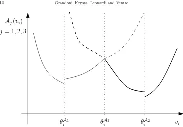
A2iFig. 1. Consider two bitonic algorithmsA1andA2. The thin (resp., thick) curves represents the objective value A1(vi)(resp., A2(vi)) returned byA1 (resp., A2) as a function of the decla-ration vi of agenti (assuming that the other declarations are fixed to some value). Consider the algorithmA3 which outputs the solution of largest value among the ones output byA1andA2. The corresponding objective valueA3(vi)is given by the dashed curve.
A3 does not assign the good to agent 1 ifv1∈[0,1/2)∪(1,3/2), and does assign the good to agent 1 ifv1∈(1/2,1). Hence the monotonicity property is not satisfied.
To handle cases like the one above, the following stronger notion of bitonicity turns out to be useful. Intuitively, for a (single-objective) maximization problem, a monotone algorithm A is bitonic (w.r.t. the objective function) if, for each agent f and fixedℓ′−f, the objective value of the solution found byA is a non-increasing
function of ℓ0(f) for ℓ0(f) < θA
f, and it is a non-decreasing function of ℓ0(f) for
ℓ0(f) ≥ θAf. This property is sufficient to guarantee a monotone (bitonic, in fact)
composition of algorithms, see Figure 1 for an intuition. In the above example,A2is bitonic. On the other hand,A1 is not bitonic: e.g., ifv2< v3, at valuev1= 1< θA11 the objective function increases. We remark that bitonicity can be also defined w.r.t. some function different from the objective function.
We now apply bitonicity to our setting. Consider a cost function c: 2U →Q+. Intuitively,c plays the same role as the objective function in the previous examples. The choice ofc will depend on the context.
Definition 2.3. Let S be the solution computed by an algorithm A with dec-larations (ℓe)
e∈U. For a vector (¯ℓe)e∈U, with ℓ−f = ¯ℓ−f and ℓ¯i(f) i ℓi(f) for all
i ∈ {0,1, . . . , k}, we let S denote the solution computed by A on input (¯ℓe)
e∈U. Al-gorithm A is bitonic with respect to a cost function c(·) if the following properties hold:
(i) If f ∈S, thenf ∈S¯ and¯c( ¯S)0c(S). (ii) If f /∈S, then either f ∈S¯or ¯c( ¯S)0c(S).
[image:10.612.74.439.73.327.2]that when agentf is not winning (f /∈S andf /∈S¯) then the costc(·) of the solution is non-increasing (as function of ℓ0(f)), and when agent f is winning (f ∈ S and f ∈S¯) then the cost c(·) of the solution is non-decreasing.
In the following, we usually letPbe the original problem and ¯P denote a problem in which f changes its declaration as in the above definition. Observe that a bitonic algorithm is monotone, while the vice versa is not necessarily true. As shown in [7], bitonic algorithms can be combined to get a monotone algorithm.
Theorem 2.4. (Composition Theorem) [7] Consider a procedure M which
generates a (potentially infinite) family of subproblems P1, P2, . . ., solves each sub-problemPi with a procedureMiand returns the solutionSito problemPi minimizing
(resp., maximizing)ci(Si), for given cost functionsci(·)(the best solution with largest
index iin case of ties). If each procedure Mi is bitonic with respect toci(·), then M
is monotone.
We remark that, although no implementable algorithm produces an infinite family of subproblems, we will need the technicality of infinitely many subproblems in the proof of a few lemmas. For more details concerning this aspect we refer the reader to [7].
In the following, we will denote byf the element whose type is modified according to the definition of monotonicity/bitonicity, and by e a generic element. We use an upper bar to denote quantities in the modified problem. ByN we denote a dummy (null) solution which is returned when no feasible solution exists. For notational convenience, we will assume that N does not contain any element, and that it has cost−∞forbest= max and +∞otherwise.
Some considerations about our model. Generalized single-minded agents adapt well to our setting. Consider again the case in which P models the BMST problem and ℓ0(f) and ℓ1(f) are respectively the cost and the delay experienced when using edgef. As noted, agentf cannot lie promising a delay smaller than her true one (or otherwise the mechanism cana posteriori verify that the agent lied). In the valuation function above, this is reflected by a valuation of−∞for declarations in which agents underbid the delay. (In other words, an agent would incur an infinite cost to provide the service with a smaller delay.) More generally, the valuation functions that we consider, model optimization problemsP in which budgeted parameters are somehow verifiable (thus implying that certain lies are irrational for a selfish agent).
Valuation function (2.1) connects with two different research areas in algorith-mic mechanism design. Mechanisms with verification, introduced by [30] and further studied in [33] (see also references therein), exploit the observation that the execu-tion of the mechanism can be used to verify agents misreporting their types (i.e., the entire type must be verifiable). On the contrary, in our framework this assumption is only made for budgeted parameters, i.e., ℓ0(·)’s can model unverifiable quantities (e.g., costs). Valuation function (2.1) expresses the valuation of single-minded bid-ders in a combinatorial auction (considered the paradigmatic problem in algorithmic mechanism design) using exact allocation algorithms. Indeed, it is enough to consider the budgeted parameter as the demand set (i.e., a bidder evaluates−∞a set which is not a superset of her unique demand set).
ℓe2 = (0,0) and ℓe3 = (0, H) for some 0 < ε ≤ L and H > L. When agents are truthtelling the VCG mechanism would select the only feasible tree comprised of edges e1ande2. The utility of edgee3 is in this case 0. Now consider edgee3 misreporting her type as follows: ℓe3
= (0, L). In this case the VCG mechanism would output the spanning tree{e2, e3}(i.e., the minimum cost tree among the seemingly feasible ones) and pay agente3an amount ofε >0. Since the true cost ofe3is 0 thene3has a strict improvement of her utility by lying. (Note that on the contrary in our generalized single-minded setting the valuation ofe3 would be−∞in this case.) VCG fails since there is a part of agents’ type (namely, the delay) whose lies are not reflected in the objective function considered by VCG (which is only the sum of the costs). Note, however, that overbidding the delay can only shrink the set of seemingly feasible solutions and thus gives no advantages to unselected agents. Indeed, as observed above VCG is truthful (though not efficient) in our generalized single-minded setting. Finally, we remark that the example described above can be tweaked to show that no algorithm with polynomially bounded approximation guarantee can be used to obtain a truthful mechanism satisfying a strict form of voluntary participation (i.e., a mechanism in which selected agents always have a strictly positive utility). It is enough to consider the same instance with ℓe1 = (M, ε) and ℓe2 = (1,0). Any M -approximation algorithm in input ℓe1, ℓe2 and ¯ℓe3 must select the tree comprised of edgese2 ande3.
We conclude that generalized single-minded agents is a general framework moti-vated by combinatorial auctions that well encompasses the multi-objective optimiza-tion problems that we consider.
3. Exact Algorithms and Monotone Multi-Criteria FPTASs. In this sec-tion we restrict our attensec-tion to multi-objective optimizasec-tion problemsP whose exact version admits a pseudo-polynomial-time algorithmA. We focus here on the case that
Ais deterministic, the randomized case being analogous. For these problems we de-scribe a monotone multi-criteria FPTAS multi. Recall that we assume that one can in polynomial time discard an element ein the sense described in the introduction. Our approach is inspired, approximation-wise, by the construction ofε-approximate Pareto sets in [32], and crucially exploits the combination of bitonic procedures to achieve monotonicity.
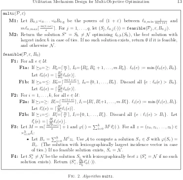
3.1. Algorithm. Algorithm multi is described in Figure 2.10. The basic idea is to generate a family of subproblemsP1, . . . ,Pq. Each subproblemPj is solved by means of a procedure feasible, hence obtaining a solution Sj and a cost function
ℓ0,j(·) (Step M1). This procedure is designed in order to be bitonic with respect
to ℓ0,j(·) on subproblem Pj. Eventually multi returns the solution Sh optimizing
ℓ0,h(Sh), thebest solution with largest indexhin case of ties (Step M2).
In more detail, letℓ0,min and ℓ0,max be the smallest and largest cost ℓ0,
respec-tively. We defineB0,1≺0. . .≺0B0,q to be all the (positive and/or negative) powers of
(1 +ε) between proper boundary values. Intuitively,B0,j is an approximate guess of
the cost of OP T. The case that OP T is empty, and hence has cost zero, is handled in Step M2. For each B0,j,Pj is the feasibility problem obtained by considering the
set of constraints of the original problemP, plus the constraintP
e∈Uℓ0(e)xe0B0,j. For a given subproblem Pj with B0 :=B0,j, procedurefeasible computes an
ε-feasible solution to Pj, i.e., a solution Sj ∈ S such that each budget constraint is
10The interested reader might initially just focus on the case that
i=≥for alli, which is probably
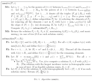
multi(P, ε)
M1: Let B0,1≺0. . .≺0B0,q be the powers of (1 + ε) between ℓ0,min 1
m(1+ε) and
m ℓ0,max⌈m(1+ε ε)⌉. Forj= 1, . . . , q, let (Sj, ℓ0,j(·)) =feasible(Pj, ε, B0,j).
M2: Return the solutionS∗ =Sh6=N optimizingℓ0,h(Sh), thebest solution with
largest indexhin case of ties. If no such solution exists, return∅if it is feasible, and otherwiseN.
feasible(P, ε, B0)
F1: For alle∈ U: F1a: If 0=≥: B′
0=⌈mε⌉,I0={B
′
0, B0′ + 1, . . . , m B0′}. ℓ0(e) := min{ℓ0(e), B0}.
Letℓ′
0(e) =⌊
B′ 0 B0ℓ0(e)⌋. F1b: If 0=≤: B0′=⌈m(1+ε)
ε ⌉,I0={0,1, . . . , B
′
0}. Discard all{e:ℓ0(e)> B0}.
Letℓ′
0(e) =⌈
B′ 0 B0ℓ0(e)⌉. F2: Fori= 1, . . . , k, for alle∈ U:
F2a: Ifi=≥:Bi′=⌈m(1+ε)
ε ⌉,Ii={B
′
i, Bi′+1, . . . , m Bi′}.ℓi(e) := min{ℓi(e), Bi}.
Letℓ′
i(e) =⌈ B′
i Biℓi(e)⌉.
F2b: If i=≤: B′
i=⌈mε⌉, Ii={0,1, . . . , B
′
i}. Discard all {e :ℓi(e) > Bi}. Let ℓ′
i(e) =⌊ B′
i Biℓi(e)⌋.
F3: LetM =m⌈m(1+ε)
ε ⌉+ 1 andϕ(·) =
Pk i=0M
iℓ′
i(·). For allz= (z0, z1, . . . , zk)∈ ×k
i=0Ii:
• LetBz=Pki=0Mizi. UseAto compute a solutionSz ∈ Swithϕ(Sz) = Bz. (The solution with lexicographically largest incidence vector in case
of ties.) If no feasible solution exists,Sz=N.
F4: LetSz∗6=N be the solutionSz with lexicographicallybest z(Sz∗=N if no such
solution exists). Return (S∗
z, B0 B′ 0ℓ
′
0(·)).
Fig. 2.Algorithmmulti.
violated at most by a factor (1 +ε). Moreover, feasible returns a cost function ℓ0,j(·) such that the behavior of feasibleis bitonic with respect to function ℓ0,j(·)
on subproblem Pj (more details in the proof of Lemma 3.2). In order to achieve this goal,feasiblefirst constructs an auxiliary feasibility problemP′
j, with lengths
ℓ′
i(e) and budgets Bi′ which are polynomially-bounded in m/ε (Steps F1 and F2).
The definitions of those auxiliary lengths and budgets are such that any feasible (w.r.t. ℓi(·), i ≥ 1) solution for Pj is feasible for Pj′, and every feasible solution
to P′
j is ε-feasible (w.r.t. ℓi(·), i≥ 1) for Pj (more details in the proof of Lemma
3.1). Then feasible finds a feasible solution forP′
j by encoding this problem in a
proper family of exact problems, which are solved by means of A (Step F3). Each exact problem is indexed by a vector z = (z0, . . . , zk) in a proper domain ×ki=0Ii.
Consider the length vector Λ(·) = (ℓ′
0(·), . . . , ℓ′k(·)). The solutionSz returned for the
exact problem indexed byz, if non-null, satisfies Λ(Sz) =z(here we exploit the fact
thatM is large enough compared to the quantitiesℓ′
i(·)). The domain ×ki=0Ii covers
all the possible feasible length vectors. Hence, if there is a feasible solution to P′ j,
i.e., a solutionSj withℓ′i(Sj)iBi′for alli, this solution will be found byfeasible.
Eventually (Step F4), among the feasible solutionsSzobtained,feasiblereturns the
[image:13.612.72.443.76.441.2]approximation ratio (due to the fact that we optimizez0 first), is crucial to enforce bitonicity.
Note that in Step F3, in case of multiple solutions of target valueB, the algorithm returns the solution of largest incidence vector. This tie breaking rule is also crucial to achieve bitonicity. It is easy to modify a given exact algorithmA to enforce this property. Lete1, e2, . . . , em be the elements, and B′ =B. For i= 1, . . . , m, we add
a very large (but still polynomial) value Lto ϕ(ei), and ask for a solution of target
value L+B′. For L large enough, any such solution must contain e
i. If no such
solution exists, we discard ei. Otherwise, we set B′ ← B′+L. In both cases we
proceed with next edge. Here we exploit the assumption that discarding one element does not change the nature of the considered problem.
3.2. Analysis. Let us bound the running time and approximation factor of
multi.
Lemma 3.1. Algorithmmulticomputes a(1+ε)2-approximate solution, violating each budget constraint at most by a factor(1 +ε). The running time of the algorithm is polynomial in the size of the input and 1/ε.
Proof. Consider the running time of feasible on a given subproblem Pj. Lengths ℓ′
i(·) and budgetsBi′ are polynomially bounded inm/ε. Consequently, the number of
exact problems generated to solveP′
jisO((m/ε)k) =O((m/ε)O(1)) sincekis constant.
Also, the fact that k = O(1) implies that the values of ϕ(·) and B of each exact problem satisfy the same bound. SinceAis a pseudo-polynomial-time algorithm, it follows that each exact problem can be solved inO((m/ε)O(1)) time. Altogether, the running time of feasible is O((m/ε)O(1)). The number of subproblems generated bymultiisO(log1+ε
m ℓ0,max
εℓ0,min ), which is polynomial in the size of the input and 1/ε.
The running time bound follows.
Consider now the approximation factor. We initially observe that the solutionS∗ returned by the algorithm violates each budget constraint at most by a factor (1 +ε). Indeed, consider any solution S returned for some subproblem P′
j and anyi≥1. If i=≥, one has:
ℓi(S) = Bi
B′ i
X
e∈S
B′ i
Bi
ℓi(e)≥ Bi
B′ i
X
e∈S
B′ i
Bi
ℓi(e)
−1
= Bi B′ i
X
e∈S
(ℓ′i(e)−1)
≥Bi−
Bi
B′ i
m=Bi−
Bim
⌈m(1 +ε)/ε⌉ ≥Bi−
Bim
m(1 +ε)/ε = Bi
(1 +ε).
Otherwise (i=≤),
ℓi(S) =
Bi
B′ i
X
e∈S
B′ i
Bi
ℓi(e)≤
Bi
B′ i
X
e∈S B′
i
Bi
ℓi(e)
+ 1
= Bi B′ i
X
e∈S
(ℓ′
i(e) + 1)
≤Bi+Bi
B′ i
m=Bi+ Bim
⌈m/ε⌉ ≤Bi+
Bim
m/ε =Bi(1 +ε).
In both cases, in the second inequality we used the feasibility ofS w.r.t. P′ j.
We next show that Sh := S∗ is (1 +ε)2-approximate. The claim is trivially
true if there is no feasible solution or the optimum solution is empty. Otherwise, let OP T 6= ∅ be an optimum solution to the original problem instance. Consider first the case that 0=≥(i.e., we are considering a maximization problem). Recall that B0,1 < . . . < B0,q are powers of (1 +ε). Let j be the largest index such that
Observe that there is one such valueB0,j, sinceℓ0,min≤ℓ0(OP T)≤m ℓ0,max. Note
that OP T is feasible forP′
j, i.e., ℓ′i(OP T)i Bi′ fori ≥0. To see this, consider an
execution of (Sj, ℓ0,j(·)) = feasible(Pj, ε, B0,j) in algorithm multi. Observe that
ℓ′
0(·) =ℓ0,j(·) B′
0,j
B0,j,B0=B0,j, and B ′
0=B0′,j. For anyi≥1,
ℓ′i(OP T) = X
e∈OP T
ℓ′i(e)i X
e∈OP T
B′ i
Bi
ℓi(e)i B ′ i
Bi
Bi=B′i.
In the first inequality above we used the fact that, ℓ′
i(e) = ⌈ B′
i
Biℓi(e)⌉ ≥ B′
i
Biℓi(e) for i=≥, and that ℓ′
i(e) = ⌊ B′
i
Biℓi(e)⌋ ≤ B′
i
Biℓi(e) otherwise. In the second inequality
above we used the fact thatOP T is feasible w.r.t. the original problem. Moreover,
ℓ′0(OP T) =
X
e∈OP T
ℓ′0(e) =
X
e∈OP T B′
0 B0ℓ0(e)
≥ X
e∈OP T
B′ 0 B0
ℓ0(e)−1≥B′0(1 +ε)−m≥B0′.
In the second inequality above we used the assumption ℓ0(OP T) ≥B0,j(1 +ε) =
B0(1 +ε). In the third inequality above we used the fact thatB′ 0=
m ε
≥mε. Since OP T is feasible, a solution Sj is returned for subproblem Pj. By the
optimality ofSh,ℓ0,h(Sh)≥ℓ0,j(Sj). It follows that
B0,h
B′ 0,h
ℓ′0,h(Sh) =ℓ0,h(Sh)≥ℓ0,j(Sj) =
B0,j
B′ 0,j
ℓ′0,j(Sj)≥B0,j>
ℓ0(OP T) (1 +ε)2 .
In the second inequality above we used the feasibility ofSj and in the last inequality
the assumptionℓ0(OP T)< B0,j(1 +ε)2. The cost ofS∗=Sh then satisfies
ℓ0(Sh) =
B0,h
B′ 0,h
X
e∈Sh
B′ 0,h
B0,h
ℓ0(e)≥B0,h
B′ 0,h
X
e∈Sh B′
0,h
B0,h
ℓ0(e)
= B0,h B′
0,h X
e∈Sh
ℓ′ 0,h(e) =
B0,h
B′ 0,h
ℓ′
0,h(Sh)>
ℓ0(OP T) (1 +ε)2 .
The case0=≤is analogous. HereB0,1 > . . . > B0,q are powers of (1 +ε), and
we let j be the largest index such that ℓ0(OP T)≤B0,j/(1 +ε) (hence ℓ0(OP T)>
B0,j+1/(1 +ε) =B0,j/(1 +ε)2. Also in this case OP T is feasible forPj′. Fori≥1,
one can show thatℓ′
i(OP T)iBi′ is the same way as in the previous case. Moreover
ℓ′
0(OP T) =
X
e∈OP T
ℓ′ 0(e) =
X
e∈OP T B′
0 B0
ℓ0(e)
≤ X
e∈OP T
B′ 0 B0
ℓ0(e) + 1≤ B ′ 0
1 +ε+m≤B
′ 0.
In the last inequality above we used the fact thatB′ 0=
lm(1+ε) ε
m
. It follows that
B0,h
B′ 0,h
ℓ′0,h(Sh) =ℓ0,h(Sh)≤ℓ0,j(Sj) =
B0,j
B′ 0,j
We can conclude that that the cost of the approximate solutionS∗=S
hsatisfies
ℓ0(Sh) =
B0,h
B′ 0,h
X
e∈Sh
B′ 0,h
B0,h
ℓ0(e)≤ B0,h
B′ 0,h
X
e∈Sh B′
0,h
B0,h
ℓ0(e)
=B0,h B′
0,h X
e∈Sh
ℓ′0,h(e)
=B0,h B′
0,h
ℓ′0,h(Sh)<ℓ0(OP T)(1 +ε)2.
We next prove the bitonicity offeasible: via the Composition Theorem 2.4 this will imply the monotonicity ofmulti.
Lemma 3.2. Procedure feasibleis bitonic with respect toℓ0,j(·)on subproblem Pj.
Proof. Consider an execution of (Sj, ℓ0,j(·)) =feasible(Pj, ε, B0,j) in algorithm
multi. Observe that ℓ′
0(·) =ℓ0,j(·) B′
0,j
B0,j, B0 =B0,j, and B ′
0 =B′0,j. Let also ¯Sj be
the solution output byfeasiblefor problem ¯Pj. Since ℓ0,j(·) = BB0′
0ℓ ′
0(·), it is sufficient to prove bitonicity with respect to ℓ′0(·). Suppose we modify ℓs(f) to ¯ℓs(f) s ℓs(f) for somes ∈ {0, . . . , k}. Observe that
this implies ¯ℓ′
s(f) s ℓ′s(f). Consider the case ¯ℓ′s(f) = ℓ′s(f): here Sj = ¯Sj and so
the algorithm is trivially bitonic. Then assume ¯ℓ′
s(f)≻s ℓ′s(f). ByF we denote the
set of feasible solutions toP′
j computed byA. Note thatF ⊆F¯, since every feasible
solution toP′
jis feasible for ¯Pj′ as well. Moreover, every solution in ¯F \F must contain
f.
For two solutions ¯S and S and two length vectors ¯Λ and Λ, recall that by def-inition ¯Λ( ¯S) Λ(S) iff, for some j ∈ {0, . . . , k}, ¯ℓ′
i( ¯S) = ℓ′i(S) for i = 0, . . . , j,
and ¯ℓ′
j+1( ¯S) ≻j+1 ℓ′j+1(S) if j < k. Consider first the case f ∈ Sj. We will
show that f ∈ S¯j and ¯Λ( ¯Sj) Λ(Sj) (which implies ¯ℓ′0( ¯Sj) 0 ℓ′0(Sj)). Note that
¯
Λ(Sj)≻Λ(Sj) since ¯ℓ′s(f)≻s ℓ′s(f). Moreover, because Sj ∈ F ⊆ F¯ and the
algo-rithm returns in Step F4 the lexicographically best solution, we have ¯Λ( ¯Sj)Λ(¯ Sj).
As a consequence, ¯Λ( ¯Sj)Λ(¯ Sj)≻Λ(Sj). On the other hand, for anyf /∈S′∈ F,
¯
Λ(S′) = Λ(S′)Λ(S
j) (where again follows from Step F4), and hence S′ 6= ¯Sj.
We can conclude thatf ∈S¯j.
Suppose now f /∈ Sj and f /∈ S¯j. We will show that ¯Sj = Sj (which implies
¯ ℓ′
0( ¯Sj)0ℓ′0(Sj)). Since all the solutions in ¯F \ F containf, ¯Sj ∈ F. Then ¯Λ( ¯Sj) =
Λ( ¯Sj)Λ(Sj) = ¯Λ(Sj)Λ( ¯¯ Sj) (where we referred to Step F4 twice), which implies
¯
Λ( ¯Sj) = Λ(Sj). Therefore the set of solutions not containing f which optimize the
length vector Λ is exactly the same in the two problems. This implies that ¯Sj =Sj
by the lexicographic optimality of the solutions computed.
Lemma 3.3. Algorithmmulti is monotone.
Proof. It is sufficient to consider the case that the solution to the original problem is not ∅ norN. Consider the variant ideal of multi which spans all the (infinitely many) powers of (1 +ε). Observe that ideal and multi output exactly the same solution (both in the original and in the modified problem). In fact, consider the case
0=≥. For B0 < ℓ0,minm , we have ℓ′0(e) =B0′ for all e, which leads to a solution of ℓ0,j cost at most BB0′
0mB ′
0 < ℓ0,min. On the other hand, for B0 > mℓ0,max⌈m(1+ε ε)⌉, we haveℓ′
0(e) = 0 for alle, which leads to a solution of ℓ0,j cost zero. Observe that
in both cases the solutions computed byidealonly are not better than the solutions computed bymulti. The case0=≤is symmetric. ForB0< ℓ0,minall the edges are
discarded and the problem becomes unfeasible. ForB0> mℓ0,max⌈m(1+ε ε)⌉, we have ℓ′
0(e) = 1 for alle, which leads to a solution of ℓ0,j cost at least BB0′
in this case the solutions computed byideal only are not better than the solutions computed also bymulti. By Lemma 3.2 and the Composition Theorem 2.4,idealis monotone. We can conclude thatmultiis monotone as well.
The deterministic part of Theorem 1.1 follows from Lemmas 2.2, 3.1, and 3.3. The randomized part of Theorem 1.1 follows analogously by observing that one can make the failure probability of each execution of A (and hence of the overall algorithm) polynomially small.
4. Lagrangian Relaxation and Budgeted Minimum Spanning Tree. In this section we investigate a different approach to the design of truthful mechanisms, based on the classical Lagrangian relaxation method. With this approach, we obtain a monotone randomized PTASbmstfor the budgeted minimum spanning tree problem (BMST). This implies a universally truthful mechanism for the corresponding game. We are also able to derandomize our PTAS in the special case of positive integer lengths.
Let us start by introducing some preliminary notions. For notational convenience, letc(·) =ℓ0(·), ℓ(·) =ℓ1(·) andL=B1. By cmin andcmax we denote the smallest
and largest cost, respectively. BMST can be defined as follows:
min X
e∈E
c(e)xe
s.t. x∈ X X
e∈E
ℓ(e)xe≤L
Here X denotes the set of incidence vectors of spanning trees of the input graph G = (V, E). For a Lagrangian multiplier λ ≥ 0, the Lagrangian relaxation of the problem is (see [35])
LAG(λ) = min X
e∈E
c(e)xe+λ·( X
e∈E
ℓ(e)xe−L)
s.t. x∈ X
The problem above is essentially a standard minimum spanning tree problem, with respect to the Lagrangian costs c′(e) = c(e) +λ ℓ(e). Observe that, for anyλ ≥0,
LAG(λ) ≤ OP T. We let λ∗ (optimal Lagrangian multiplier) be a value of λ ≥ 0 which maximizes LAG(λ). In case of a tie, we let λ∗ be the smallest such value. If
λ∗=∞, there is no feasible solution. We remark thatλ∗can be computed in strongly-polynomial-time, using, say, Megiddo’s parametric search technique (see, e.g., [35]).
Function LAG(λ) has a natural geometric interpretation. For any spanning tree S with incidence vectorx(S),cλ(S) :=Pe∈Ec(e)xe(S) +λ·(Pe∈Eℓ(e)xe(S)−L) is
a linear function of the multiplierλ. The slope ofcλ(S) is positive ifS is unfeasible,
and non-positive otherwise. LAG(λ) is the lower envelope of the linescλ(S), forλ≥0
and S ∈ S. Observe that LAG(λ) is concave and piecewise linear. We will refer to cλ(S) as theline associated toS. When no confusion is possible, we will sometimes
use the notion of spanning tree and of the corresponding line interchangeably. We observe the following useful fact.
Lemma 4.1. Consider the lower envelope LE of the lines of a set of solutions. Letcλ(S1), cλ(S2), . . . , cλ(Sq)be the lines intersectingLE, sorted in decreasing order
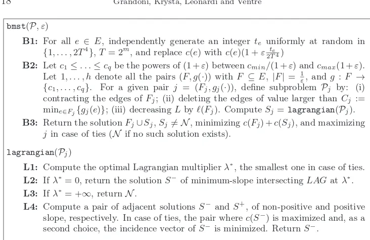
bmst(P, ε)
B1: For all e ∈ E, independently generate an integer te uniformly at random in {1, . . . ,2T4},T= 2m, and replacec(e) withc(e)(1 +ε te
2T4)
B2: Letc1≤. . .≤cqbe the powers of (1 +ε) betweencmin/(1 +ε) andcmax(1 +ε).
Let 1, . . . , hdenote all the pairs (F, g(·)) with F ⊆E,|F|= 1
ε, and g:F → {c1, . . . , cq}. For a given pair j = (Fj, gj(·)), define subproblem Pj by: (i)
contracting the edges ofFj; (ii) deleting the edges of value larger thanCj :=
mine∈Fj{gj(e)}; (iii) decreasingLbyℓ(Fj). ComputeSj=lagrangian(Pj).
B3: Return the solutionFj∪Sj,Sj6=N, minimizingc(Fj) +c(Sj), and maximizing jin case of ties (N if no such solution exists).
lagrangian(Pj)
L1: Compute the optimal Lagrangian multiplierλ∗, the smallest one in case of ties. L2: Ifλ∗= 0, return the solutionS−of minimum-slope intersectingLAGatλ∗. L3: Ifλ∗= +∞, returnN.
L4: Compute a pair of adjacent solutionsS−andS+, of non-positive and positive
slope, respectively. In case of ties, the pair wherec(S−) is maximized and, as a
second choice, the incidence vector ofS−is minimized. ReturnS−.
Fig. 3.Algorithmbmst.
Proof. It is sufficient to show that, for anyi= 1,2, . . . , q−1,c(Si)≤c(Si+1). If lines Si and Si+1 overlap, the claim is trivially true since in that case c(Si) = c(Si+1). Otherwise, letλ′be the value ofλfor whichc
λ′(Si) =cλ′(Si+1) (the two lines cannot be parallel, since they both intersectLE).Recall thatℓ(Si)≥ℓ(Si+1) by assumption. Then
c(Si) =cλ′(Si)−λ′(ℓ(Si)−L)≤cλ′(Si)−λ′(ℓ(Si+1)−L) =cλ′(Si+1)−λ′(ℓ(Si+1)−L) =c(Si+1).
4.1. Algorithm. Algorithm bmst is described in Figure 3. Let ε∈ (0,1] be a given constant parameter. W.l.o.g., we can assume that the graph contains at least 2 + 1/ε nodes (and hence any spanning tree at least 1 + 1/ε edges). Otherwise, we can solve the problem optimally in polynomial time by brute force. Furthermore, the brute force algorithm can be easily made monotone with a careful implementation. The algorithm initially randomly perturbs the edge costs (Step B1). The factorT = 2m in the perturbation is simply an upper bound on the number of spanning trees.
Our perturbation will ensure, with high probability, that no more than two lines corresponding to spanning trees intersect at any given point.
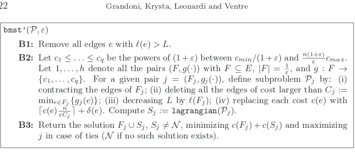
Then (Step B2), the algorithm generates a polynomial set of subproblems P1,
P2, . . . ,Ph. Intuitively, each subproblem corresponds to a guess of the most expensive edges in the optimum solutionOP T, and to a guess of their approximate cost. More precisely, each subproblem j is labeled by a pair (Fj, gj(·)), whereFj is a subset of
1/ε edges, and gj : Fj → C, where C = {c1, . . . , cq} is a proper set of powers of
(1 +ε). Given a pairj= (Fj, gj(·)), subproblemPj is obtained by contracting edges
Fj, deleting all the edges of cost larger than Cj := mine∈Fj{gj(e)}, and decreasing
[image:18.612.71.437.78.315.2]Each subproblem Pj is solved by means of a procedurelagrangian, based on the Lagrangian relaxation method. In particular, following [35], among the solutions intersectingLAGatλ∗, we select two adjacent solutionsS− andS+, of non-positive and positive slope respectively, and return Sj = S−. We recall that two spanning
treesS− andS+are adjacent in the spanning tree polytope if there are edgese+and e− such thatS− =S+\ {e+} ∪ {e−}. As mentioned in the introduction, in case of ties we select the pair (S−, S+) with maximumc(S−).
Eventually (Step B3), bmst returns the (feasible) solution Fj∪Sj of minimum
costc(Fj∪Sj) =c(Fj) +c(Sj) (and largest indexj in case of ties).
4.2. Analysis. We remark that the values te in the perturbation are
indepen-dent from edge costs and lengths, and hence we can assume that they are the same in the original (Pj) and modified ( ¯Pj) problems. In other words, each choice of the te’s specifies one deterministic algorithm. We will show that each such algorithm
is monotone. Note also that monotonicity on the perturbed instance implies mono-tonicity on the original instance, since the perturbation does not change the sign of the difference between modified and original costs/lengths. As a consequence, the resulting mechanism will be universally truthful. The random perturbation has the following property.
Lemma 4.2. After the perturbation, with probability at least 1−1/T, all the spanning trees correspond to different lines, and at most two lines intersect at a given point.
Proof. Consider any two lines S1 and S2, and let ℓi and ci be the length and
perturbed cost of Si, respectively. The two lines overlap if and only if c1 =c2 and ℓ1 =ℓ2. Let us condition over the cost of all the edges of S1 and of all the edges of S2but one. Thenc2 is a random variable which takes one value uniformly at random in a set of 2T4 distinct values. Hence the event{c
1 =c2} happens with probability at most 1/2T4.
Consider now any three lines S1, S2 and S3. With the same notation as above, these three lines intersect at the same point if and only if
(
c1+λ(ℓ1−L) =c2+λ(ℓ2−L) c1+λ(ℓ1−L) =c3+λ(ℓ3−L),
for some valueλ≥0. Ifℓ1=ℓ2, it must bec1=c2which happens with probability at most 1/2T4by the same argument as before. Otherwise it must bec3=c1+λ(ℓ1−ℓ3) withλ= (c1−c2)/(ℓ2−ℓ1): this happens with probability at most 1/2T4by a similar argument.
Since there are at mostT2 pairs and T3 triples of the kind above, by the union bound the probability that the property of the claim is not satisfied is at most T2/(2T4) +T3/(2T4)≤1/T.
Lemma 4.2 immediately implies that, with high probability, there are exactly two solutions of optimal Lagrangian cost. This will be crucial to prove that the running time ofbmstis polynomial in expectation.
The following lemma bounds the approximation guarantee and efficiency of algo-rithmbmst.
Lemma 4.3. For any fixedε∈(0,1], the expected running time of algorithmbmst
is polynomial.
Proof. The perturbation can be performed inO(mlog(2T4)) =O(m2) time. Al-gorithm bmstruns at mostO((mlog1+εccmaxmin)
polynomial in the input size for any constantε >0. The running time oflagrangian
is dominated, modulo polynomial factors, by the number of spanning trees of optimal Lagrangian cost for the considered instance. This number is at mostT deterministi-cally, and it is exactly 2 with probability at least (1−1/T) by Lemma 4.2. Hence the expected running time oflagrangianis polynomial.
Lemma 4.4. For any fixedε∈(0,1], algorithmbmst is(1 + 5ε)-approximate. Proof. The algorithm can only return feasible solutions. Let us assume that a feasible solution exists, otherwise there is nothing to prove. Let OP T be the op-timum solution to the perturbed instance, and F the 1/ε most expensive edges in OP T. Consider the assignment g : F → {c1, . . . , cq} such that, for each e ∈ F,
g(e) ≥ c(e) ≥ g(e)/(1 +ε). Let OP T′ and OP T′′ be the optimum solution to the subproblems induced by j = (F, g(·)) and (F, c|F(·)), respectively. Observe that c(OP T′′) =c(OP T)−c(F). Moreover, c(OP T′)≤c(OP T′′) since mine∈F{c(e)} ≤
mine∈F{g(e)} (intuitively, for a given guess F we prune more edges with c(·) than
withg(·)). Altogether c(OP T′)≤c(OP T)−c(F). Note also that in subproblemPj each edgeecosts at mostε(1 +ε)c(OP T). Ifλ∗= 0, c(S−) =c(OP T′). Otherwise
c(S−) =c(S+) +c(e−)−c(e+)≤LAG(λ∗) +c(e−)
≤c(OP T′) +c(e−)
≤c(OP T′) +ε(1 +ε)c(OP T).
It follows that c(F) +c(S−)≤c(OP T) +ε(1 +ε)c(OP T). It is easy to see that the initial perturbation increases the cost of the optimal solution at most by a factor (1+ε) (deterministically). Thus the overall approximation factor is (1 +ε)(1 +ε(1 +ε))≤
1 + 5ε.
It remains to prove thatbmstis monotone. To that aim, we start by proving the bitonicity of the subroutinelagrangian.
Lemma 4.5. Algorithmlagrangian is bitonic with respect toc(·).
Proof. By the concavity ofLAG, if λ∗ = 0, then observe that ¯λ∗ = 0 and the solution returned in the original and modified problems is exactly the same, since the line of minimum-slope output in the original problem (cf. Step L2), will have minimum slope also in the modified instance. On the other hand, forλ∗ = +∞ no solution is returned for the original problem. We note also that if cost and length off are unmodified then the algorithm returns the same solution in the original and modified problems. In all these caseslagrangian is trivially bitonic. Hence assume that 0 < λ∗ < +∞ and that f modifies either cost or length. We distinguish two cases:
(i) Case f ∈ S−: We have to show that f ∈ S¯− and ¯c( ¯S−) ≤ c(S−). Note that ¯
cλ∗(S−) is either equal tocλ∗(S−)−∆<¯cλ∗(S−) or tocλ∗(S−)−λ∗∆<¯cλ∗(S−), de-pending on whether the cost or length off is modified (decreased) by ∆, respectively. For any S 6∋ f, ¯cλ∗(S) =cλ∗(S) ≥ cλ∗(S−). (The last inequality follows from the fact that point (λ∗, c
λ∗(S−)) belongs to the lower envelope LAGand that the lower envelope is defined as the point-wise minimum of all linescλ(S) for all spanning trees
S.) HenceLAGintersects atλ∗only solutions containingf in the modified problem: sinceS− is one of those solutions, the concavity ofLAGimplies that ¯λ∗≤λ∗.