Optimal Planning with State Constraints
Franc Ivankovic
June 2017
A thesis submitted for the degree of Doctor of Philosophy
The Australian National University
c
Declaration
Except where otherwise indicated, this thesis is my own original work.
Franc Ivankovic June 2017
Acknowledgements
I am deeply grateful to my supervisor Patrik Haslum, for his support and his limitless patience. I am very thankful for all the discussions that we had and the time spent on reviewing my work.
I also want to thank: Sylvie Thi´ebaux for all her help and useful sug-gestions; the other people I worked with on papers, Dana Nau, Miquel Ramirez, and Vikas Shivashankar; other researchers at Data61 and ANU for sharing their knowledge and ideas, including Menkes van den Briel, Enrico Scala, Alban Grastien, Hassan Hijazi, Tommaso Urli, Charles Gretton, Dan Gordon, Phil Kilby, Michael Norrish; my fellow students Josh Bax, Ksenia Bestuzheva, Cody Christopher, Jing Cui, Karsten Lehmann, Boonping Lim, Terrence Mak, Mohammad Abdulaziz, Paul Scott, Fazlul Hasan Siddiqui and Frank Su; and others who worked at ANU or Data61.
Finally, I thank my friends, my family (parents, brothers, grandparents...) and Jessica for their support and encouragement.
Abstract
In the classical planning model, state variables are assigned values in the initial state and remain unchanged unless explicitly affected by action effects. However, some properties of states are more naturally modelled not as direct effects of actions but instead as derived, in each state, from the primary variables via a set of rules. We refer to those rules as state constraints. The two types of state constraints that will be discussed here are numeric state constraints and logical rules that we will refer to as axioms.
When using state constraints we make a distinction between primary variables, whose values are directly affected by action effects, and secondary variables, whose values are determined by state constraints. While primary variables have finite and discrete domains, as in classical planning, there is no such requirement for secondary variables. For example, using numeric state constraints allows us to have secondary variables whose values are real numbers. We show that state constraints are a construct that lets us combine classical planning methods with specialised solvers developed for other types of problems. For example, introducing numeric state constraints enables us to apply planning techniques in domains involving interconnected physical systems, such as power networks.
To solve these types of problems optimally, we adapt commonly used methods from optimal classical planning, namely state-space search guided by admissible heuristics. In heuristics based on monotonic relaxation, the idea is that in a relaxed state each variable assumes a set of values instead of just a single value. With state constraints, the challenge becomes to evaluate the conditions, such as goals and action preconditions, that involve secondary variables. We employ consistency checking tools to evaluate whether these conditions are satisfied in the relaxed state. In our work with numerical constraints we use linear programming, while with axioms we use answer set programming and three value semantics. This allows us to build a relaxed planning graph and compute constraint-aware version of heuristics based on monotonic relaxation.
We also adapt pattern database heuristics. We notice that an abstract
state can be thought of as a state in the monotonic relaxation in which the variables in the pattern hold only one value, while the variables not in the pattern simultaneously hold all the values in their domains. This means that we can apply the same technique for evaluating conditions on secondary variables as we did for the monotonic relaxation and build pattern databases similarly as it is done in classical planning.
To make better use of our heuristics, we modify the A? algorithm by combining two techniques that were previously used independently – par-tial expansion and preferred operators. Our modified algorithm, which we call PrefPEA?, is most beneficial in cases where heuristic is expensive to
Contents
1 Introduction 1
1.1 State constraints . . . 2
1.1.1 Contribution . . . 3
1.2 Optimal planning . . . 3
1.2.1 Contribution . . . 5
1.3 Thesis Outline . . . 7
1.4 List of publications . . . 8
2 Background 9 2.1 Classical planning . . . 10
2.1.1 Finite domain representation . . . 13
2.2 Optimal planning . . . 15
2.2.1 Monotonic Relaxation . . . 15
2.2.2 Relaxation-based heuristics . . . 17
2.2.3 Abstraction-based heuristics . . . 22
2.3 State constraints . . . 23
2.3.1 Axioms in PDDL . . . 24
2.3.2 Other uses of state constraints in discrete domains . . . 25
2.3.3 State validity . . . 26
2.3.4 Interconnected physical systems . . . 28
2.3.5 Hybrid systems . . . 31
2.4 Semantic attachments and PMT . . . 33
2.4.1 Semantic attachments . . . 33
2.4.2 Planning modulo theories . . . 35
2.4.3 Heuristics in semantic attachments and PMT planners 36 3 Numeric state constraints 39 3.1 Motivation . . . 39
3.2 Formalism . . . 40
3.2.1 State . . . 40
3.2.2 Planning problem . . . 41
3.2.3 Switched constraints . . . 42
3.2.4 Partitioned condition . . . 44
3.2.5 Actions . . . 45
3.2.6 Plans . . . 46
3.3 Domain examples . . . 47
3.3.1 Hydraulic blocks world . . . 47
3.3.2 Switching Problems in Power Networks . . . 50
3.3.3 Multi-commodity Long-haul Transportation . . . 56
3.3.4 The Counters Domain . . . 57
3.4 Expressivity . . . 58
3.4.1 Example . . . 60
3.5 Computing Heuristics . . . 62
3.5.1 Monotone relaxations . . . 62
3.5.2 Abstraction-based heuristics . . . 72
3.5.3 Computation of hmax . . . 72
3.5.4 Computation of h+ . . . 75
3.5.5 A weaker approximation of h+ . . . 77
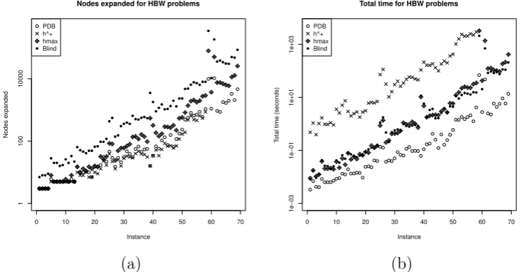
3.6 Experiments . . . 78
3.7 Future work . . . 81
4 State-dependent action costs 83 4.1 Related work . . . 84
4.2 Formalism . . . 85
4.2.1 Cases where all the extended states have the same cost 87 4.3 Computing heuristics . . . 88
4.4 Experiments . . . 89
4.5 Future work . . . 90
5 Axioms 93 5.1 Motivation . . . 93
5.2 Formalism . . . 94
5.2.1 Axioms in FDR . . . 94
5.2.2 Planning problem with axioms . . . 96
5.2.3 Axioms in PDDL . . . 98
5.2.4 Comparison with numeric state constraints . . . 99
5.3 Modelling with Axioms . . . 99
5.3.1 Min-Cut . . . 100
5.3.2 Sokoban . . . 101
5.4 Pseudo-adversarial domains . . . 103
5.4.1 Controller verification . . . 103
CONTENTS xi
5.5 Social and multi-agent planning . . . 109
5.5.1 Chang and Soo . . . 109
5.5.2 Kominis and Geffner . . . 110
5.6 Computing heuristics . . . 112
5.6.1 Naive relaxation . . . 112
5.6.2 Axiom-aware relaxations . . . 113
5.6.3 Consistency-based monotonic relaxation . . . 114
5.6.4 Consistency-based abstraction . . . 115
5.6.5 Exploring weaker relaxations . . . 116
5.6.6 Extending the relaxations to discrete finite domain sec-ondary variables . . . 117
5.7 Experiments . . . 118
5.7.1 Sokoban . . . 120
5.7.2 Controller verification . . . 120
5.7.3 Experiments with weaker relaxations . . . 121
6 Preferred operators 123 6.1 Background . . . 124
6.1.1 Preferred actions in non-optimal search . . . 124
6.1.2 A? with partial expansion . . . 124
6.1.3 PEA? with selective node generation . . . 125
6.2 Algorithm . . . 126
6.3 Experiments . . . 127
6.4 Related work . . . 129
6.5 Future work . . . 131
7 Conclusion 133 7.1 Alternative frameworks and future work . . . 134
A Proofs 135 A.1 Proposition 1 . . . 135
A.2 Proposition 2 . . . 135
B Domains 139 B.1 Min-cut . . . 139
B.2 Sokoban . . . 140
B.3 Controller verification . . . 141
B.4 Blocker . . . 143
List of Figures
1.1 Deriving heuristics . . . 6
3.1 Hydraulic Blocks World . . . 48
3.2 Deriving heuristics . . . 61
3.3 The states . . . 62
3.4 Relaxed planning graph . . . 74
3.5 Iterative Landmark Algorithm . . . 76
3.6 Disjoint Landmark Algorithm . . . 77
3.7 HBW experiments . . . 78
3.8 Counters experiments . . . 79
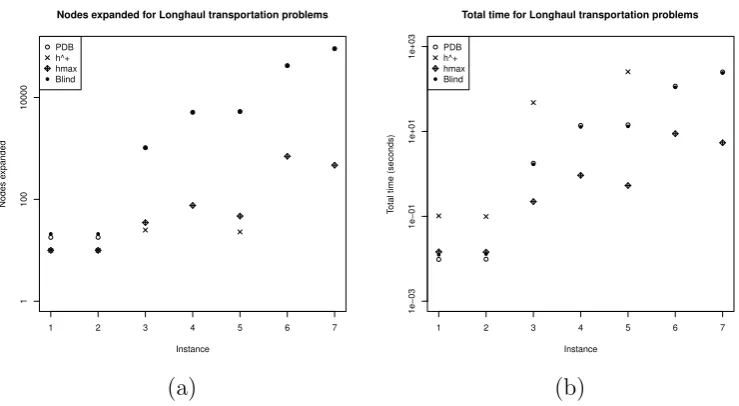
3.9 Longhaul experiments . . . 79
3.10 Problems solved . . . 80
4.1 Accuracy of h+ heuristic with unit costs and state-dependent costs . . . 90
5.1 Evaluating axioms . . . 96
5.2 The Min-Cut domain . . . 101
5.3 Sokoban . . . 104
5.4 Blocker domain . . . 105
5.5 Three value semantics . . . 117
5.6 Results – comparison of formulations with and without axioms 118 5.7 Results – nodes expanded and total time . . . 119
6.1 PrefPEA? Algorithm . . . 128
6.2 Illustration of PrefPEA? . . . 129
6.3 Results –PrefPEA? . . . 130
Chapter 1
Introduction
Planning is one of the oldest subareas of artificial intelligence, originating in the early 1960s, with the goal of achieving human-like problem solving capabilities [80, 110]. A planning task consists of an initial state the world is in, a specification of what we want to achieve, or goal, and a list of actions that are available. A solution to the planning problem, called a plan, is a sequence of actions that transforms the world from the initial state into one of the goal states.
In the classical planning model, action effects are explicitly given for each of the actions, so determining the way the world is affected by the action is straightforward. When an action is applied, the variables that do not appear in action effects retain the same value as in the previous state. However, some properties of states are more naturally modelled not as direct effects of actions but instead as derived, in each state, from the primary variables according to a set of rules that apply to all states. We call those rules state constraints.
This work focuses on optimal planning with state constraints, which we will employ for a number of purposes. We will use state constraints to ele-gantly model laws of physics in interconnected systems, such as power net-works. In these domains, the planning agent manipulates the system through discrete control actions, such as opening or closing of the switches, yet each action leads to a complicated interaction between elements of the system that depends on the state of the entire network. We will show how usage of state constraints makes some domains, such as controller verification or Sokoban, easier to solve. In order to reason about state constraints, we will integrate planners with systems used to reason about constraints, such as a linear programming solver. We will describe the way we adapted techniques commonly used in planning, namely admissible heuristics, to this setting.
1.1
State constraints
In this section, we will give an overview of general properties of state con-straints, describe some ways they can be used and introduce some terms that will appear throughout this thesis.
When using state constraints, we make a distinction between state vari-ables that are directly affected by action effects, called primary variables, and the variables whose values are determined by state constraints, called secondary variables. Conditions such as goals and action preconditions can depend on both primary and secondary variables. Constraints and secondary variables may take many different forms – for example, secondary variables may be numeric, in which case the constraints may take form of linear in-equalities, as we will see in Chapter 3.
Following Helmert’s [77] terminology, we refer to the assignment of pri-mary variables as state and an assignment of both primary and secondary variables asextended state. The assignment ofonly primary variables is sim-ply called a state, or areduced state. The relationship between a state and an extended state depends on the types of constraints that are being used. In some cases, there is always a unique assignment of secondary variables given an assignment of primary variables, in which case there is one extended state corresponding to every state. In other cases, we might have a multiple or an infinite number of extended states corresponding to a single state.
In addition to being used to compute values of secondary variables, intro-ducing state constraints allows us to make a distinction between valid and invalid states. A valid state is a state in which there is at least one assign-ment of secondary variables that satisfies all of the constraints exists. In an invalid state, it is not possible to come up with such an assignment. A plan is a sequence of actions that visits only valid states. In this setting, applying an action might not be allowed, not because any of the preconditions are unsatisfied, but because effects of the actions lead to an assignment of val-ues to primary variables that results in an invalid state. Thus, determining whether an action is applicable in a given state does not only involve check-ing whether the preconditions are satisfied, but also whether the resultcheck-ing assignment of variables constitutes a valid state.
1.2. OPTIMAL PLANNING 3
1.1.1
Contribution
The two types of state constraints that we will discuss in our work are numeric state constraints and axioms.
• Numeric state constraints allow us to use real numbers as secondary variables. As in classical planning, the primary variables are discrete. For a given assignment of primary variables, there could either be a unique assignment of secondary variables, or there could be multiple or infinitely many such assignments, or there could be none. If there is no assignment satisfying the constraints, the state is invalid.
• Axioms take the form of rules of a logic problem. Unlike in planning with numeric constraints, both primary and secondary variables have discrete domains. Another difference from planning with numeric con-straints is that given an assignment of primary variables, a unique as-signment of secondary variables satisfying the constraints is guaranteed to exist – i.e. there are no invalid states.
We use state constraints as a construct that enables us to combine clas-sical planning techniques with specialised solvers developed for other types of problems. In the case of numeric constraints, this is a linear programming solver. This widens the types of domains that can be addressed. For instance, numeric constraints allow us to apply planning techniques to problems in-volving interconnected physical systems. An example that we will return to several times throughout this thesis is power network reconfiguration problem (see Section 3.3.2).
We also show that state constraints can be used to make some domains, previously studied in classical planning, easier to model and solve. With axioms, modelling domains becomes more compact and easier to understand. In some domains, namely Sokoban (Section 5.3.2) and controller verification (Section 5.4.1), use of axioms eliminates some unnecessary choices from the planner therefore reducing the search space.
1.2
Optimal planning
The reason for this is that in many of the domains that we consider, it is beneficial to have plans that are as cheap as possible. In power network re-configuration, this is because leaving portions of the network without power is economically costly for power companies, so the process needs to be com-pleted as quickly as possible. In the controller verification domain, where finding a plan is equivalent to finding a fault in the controller, generating op-timal plans is not necessary. However, plans that are cheaper, and therefore shorter and simpler, are easier to understand. This makes fixing the faults in the controller simpler as well.
The technique commonly used in optimal planning is heuristic state-space search. This means that a search algorithm, such as A?[111] is used together
with a heuristic that determines which nodes (which represent states of the planning problem) to expand. The heuristic estimates cost of reaching the nearest goal state from the state being evaluated. A heuristic that never overestimates this cost is known as admissible heuristic. The interest in admissible heuristics is due the fact that there are search algorithms, such as already mentioned A?, which are guaranteed to return an optimal plan if
the heuristic has this property.
Domshlak and Helmert [79] give an overview of heuristics used in classi-cal planning. They categorise the heuristics as based on one of four ideas: delete relaxation, critical paths, abstractions and landmarks. In this work, we use and adapthmaxandh+, which belongs to the first category, the pattern
database heuristic, which is a form of abstraction, and our disjoint landmark heuristic (which combines ideas from delete relaxation and landmarks). As we are interested in optimal planning we limit ourselves to admissible heuris-tics.
Most of the time we will deal with cost functions that only depend on actions – that is, actions have constant costs regardless of the state in which they are applied. The cost of the plan is then simply the sum of the costs of the actions making up the plan. In most domains that we will consider, all the actions are assigned equal cost and the objective simply becomes minimising the plan length.
1.2. OPTIMAL PLANNING 5
1.2.1
Contribution
While axioms and various forms of numeric state constraints have been in-vestigated by other researchers 1, optimal planning in this setting has been neglected.
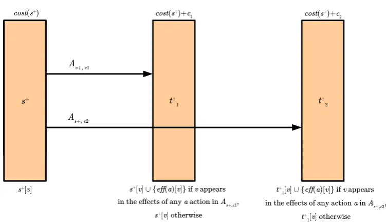
Our contribution is adapting the admissible heuristics used in classical planning to this setting. We base our approach on the idea of monotonic relaxation (Section 2.2.1). The idea is that in a relaxed state, each vari-able assumes a set of values instead of just a single value. The central challenge is to evaluate the conditions (i.e. action precondition or goals) that involve secondary variables in a relaxed state. This is approached as a consistency checking problem – using consistency checking techniques we determine whether there exists an assignment of secondary variables that satisfies the constraints and the condition that we are testing. In our work with numerical constraints, we use linear programming. With axioms, we use answer set programming and three value semantics.
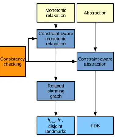
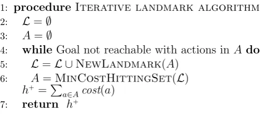
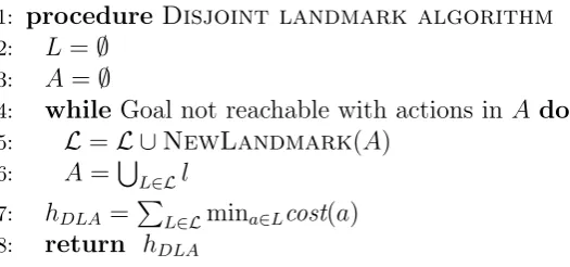
The diagram in Figure 1.1 summarises our approach. The ability to evaluate conditions on secondary variables allows us to formulate constraint-aware monotonic relaxation, which allows us to build a relaxed planning graph, hence allowing us to compute the hmax heuristic. The relaxed
plan-ning graph also provides us with relaxed reachability testing, which we use together with the iterative landmark algorithm [74] to computeh+.
Modify-ing this algorithm to generate disjoint landmarks also enables us to compute a weaker heuristic, equivalent to LM-cut for unit cost actions.
Projection (Section 2.2.3) is an abstraction that works by removing some subset of (primary) variables from the problem. The remaining (primary) variables are called a pattern. This type of abstract state can be though of as a relaxed state in which the variables in the pattern have a single value, while the primary variables not in the pattern simultaneously hold all the values in their domain. We can then employ the same consistency checking procedures as before to evaluate the conditions involving secondary variables. We use the abstraction of the problem to compute pattern databases heuris-tics (PDBs). We do this in a very similar way as it done in planning without state constraints.
Besides adapting heuristics for problems with state constraints, we also investigated planning with state dependent action costs. We discuss the issues arising from having a cost function that is dependent on an extended state. We adapt the h+ heuristic to deal with state-dependent action costs.
1For more information on axioms see Th´eibaux et al. [136] and Chapter 2. While
Consistency
checking
Constraint-aware
monotonic
relaxation
Constraint-aware
abstraction
Monotonic
relaxation
Abstraction
Relaxed
planning
graph
h
max,
h
+,
disjoint
landmarks
[image:20.595.132.510.180.630.2]PDB
1.3. THESIS OUTLINE 7
We also modified the A? algorithm by combining two techniques that were
previously used independently – partial expansion and preferred operators. The requirement is that the heuristic that we are using needs to return a list of preferred operators – in case of h+, this is a set of actions that make up
the optimal relaxed plan. Our technique, which we callPrefPEA?, is most
beneficial in cases where heuristic is expensive to compute, but accurate, and states have many successors. This applies to, for example, our power network reconfiguration domain, there are as many successors to each state as there are switches on the network.
1.3
Thesis Outline
This thesis is structured as follows:
• Chapter 2 will give an overview of background and related work. It will introduce the definitions and the notation that we will use throughout this thesis. We will then explain the techniques used in classical plan-ning that we adapted for planplan-ning with state constraints. We will also give an overview of the related work in planning with state constraints.
• Chapter 3 deals with a specific type of state constraints, namely nu-meric state constraints. We will show how we adapted heuristics in-troduced in Chapter 2 to this setting and present the domains that we used in our experiments.
• Chapter 4 will investigate state-dependent action costs in optimal plan-ning with numeric constraints.
• Chapter 5 will cover optimal planning with axioms – again, we will show how we adapted the well-known heuristics to this setting and present domains that can be modelled using axioms. We will demonstrate that axioms can make certain domains both easier to model and easier to solve.
• Chapter 6 deals with an algorithm that we developed to improve A?
search when an informative, but expensive heuristic is used. We will discuss the related work, present the PrefPEA? algorithm and the
experimental results.
1.4
List of publications
Parts of the material in this thesis has previously appeared in the following papers:
• Franc Ivankovic, Patrik Haslum, Sylvie Thi´ebaux, Vikas Shivashankar, and Dana S. Nau. Optimal planning with global numerical state con-straints. InProceedings of the Twenty-Fourth International Conference on Automated Planning and Scheduling, ICAPS 2014, Portsmouth, New Hampshire, USA, June 21-26, 2014, 2014.
• Franc Ivankovic and Patrik Haslum. Optimal planning with axioms. In Proceedings of the Twenty-Fourth International Joint Conference on Artificial Intelligence, IJCAI 2015, Buenos Aires, Argentina, July 25-31, 2015, pages 1580–1586, 2015.
Chapter 2
Background and related work
In the previous chapter we mentioned that introduction of state constraints leads to a distinction between primary and secondary variables. While a (very few) planners capable of dealing both with hybrid (a mix of real-valued and discrete) state variables and global constraints exist, in this thesis we will focus on cases where the primary variables have discrete and finite domains. In that sense, our work either meets the definition of classical planning or is only a small step away from it. To generate optimal plans we adapt techniques that were proven successful in optimal classical planning, namely state-space search guided by an admissible heuristic. In this chapter, we will give a definition of classical planning and describe the admissible heuristics commonly used in this setting. This chapter will also give an overview of the related work.
The organisation of the chapter is as follows. Section 2.1 gives a defi-nition of classical planning and highlights some of its limiting assumptions. Terminology and notation used in classical planning will be defined in this section. In subsequent chapters we will build on the formalism introduced here to formally describe planning with state constraints. In section 2.2 we will focus on techniques used for optimal planning in the classical setting. We will discuss heuristics based on monotonic relaxation and abstractions. Section 2.3 focuses on existing work on planning with state constraints. This will cover their use in domains with discrete-valued variables, their use in modelling interconnected physical systems and hybrid domains. Section 2.4 discusses the relation of state constraints to semantic attachments and plan-ning modulo theories (PMT).
2.1
Classical planning
Planning requires a formal statement, or model, of the problem. Here we will discuss the classical planning model first and then highlight some of its limiting assumptions. We will discuss how these assumptions relate to our work.
Planning is a state-transformation problem. A planning problem consists of a finite number of variables, each associated with a domain of possible values. A state is a full valuation over the variables. Actions assign new values to a subset of variables and therefore cause transitions between the states. Additionally, planning problems have agoal which is usually defined as a valuation over a subset of variables. A plan is a sequence of actions that transforms an initial state into a state in which the goal is satisfied. A planning agent is required to come up with such a sequence of actions.
The type of planning that has been most extensively studied is classical planning. This area deals with a deterministic, static, finite and fully observ-able state-transition system with restricted goals and implicit time. While classical planning has been a very active and prolific field of research, its limiting assumptions preclude us from dealing with real-world domains that cannot be modelled this way [83]. As these restrictions often make formula-tion of real world problems either impractical or impossible, there has been an interest in relaxing them or removing them. The following list of assump-tions in classical planning is adapted from Ghallab et al. [107]. In classical planning:
1. The set of states isfinite. For the state-space to be finite, every variable that we are dealing with needs to have a finite domain. Removing this restriction is necessary when dealing with numerical state variables. Real-world domains might require us to consider continuous variables such as time, velocities, positions, and keeping track of resources such as money or fuel [32]. A number of planners that we will discuss in Sections 2.3 and 2.4 are capable of dealing with numeric state variables. For a detailed overview see Coles et al. [32].
2.1. CLASSICAL PLANNING 11
3. The system isdeterministic. Applying an action in a given state brings the system to a single other (predetermined) state. In contrast, by plan-ning under uncertainty, we mean domains in which applying an action may lead to a number of different states (and which state we end up in is non-deterministic). A way to deal with this sort of problems is contingency planning, meaning that some branches are executed condi-tionally, based on the outcome of the sensory actions. Techniques that have been employed to deal with non-determinism include Markov De-cision Processes (MDPs) [22,37,88] and planning as model checking [8]. If Assumption 2 is removed as well, this leads to further difficulty as the system does not know exactly the current state of the system at run time. Dealing with this sort of problems is calledconformant plan-ning [67, 131]. The aim becomes to develop non-conditional plans that do not rely on sensory information, but still succeed no matter which state the world is actually in. For an overview of approaches to confor-mant planning see Palacios and Geffner [112].
4. The system is static, meaning that it stays in the same state until an action is applied. If a non static (or dynamic) system is deterministic and fully observable, it can easily be mapped into the static system – i.e. the planning agent knows whichevents will occur in any given state and how the occuring events alter the values of variables. It then simply becomes a modelling choice whether these changes will be described as effects of actions or effects of deterministic events, so relaxing this assumption is not interesting on its own. PDDL+ [50] is an exaple of a modelling language that allows for events and processes controlled by nature, while TM-LPSAT [129] and COLIN [32] are examples of planners that can deal with those features.
5. The planner handles only restricted goals, meaning that the objective is to find any sequence of actions that ends in a goal state. Extended goals means that we put restrictions not only on the final state, but also on states visited by a plan – this means, for example, specifying states that must be visited, states to be avoided, values that must be maintained once achieved etc. Work on preventing plans from visiting some states by Weld and Etzioni [140] that we will discuss in Section 2.3.3 is one of the simple examples. We will discuss the meaning of state validity in our setting in Chapter 3. It should be noted that in many cases, domains with extended goals can be reformulated as classical planning domains. 1
6. A solution to a planning problem is a linearly ordered finite sequence of actions. Relaxing this assumption is often necessary when some of the other assumptions are relaxed (e.g. when we are dealing with non-deterministic systems). Removing this restriction enables us to present solutions with “richer” mathematical structure. One example is already mentioned contingency planning. Alternatively, a solution might be a partially ordered set of actions or a sequence of sets. This sort of solutions are generated by partial order planners such as UCPOP [113].
7. Time not explicitly defined – actions are instantaneous state transi-tions. Plan consists of a sequence of actions, but we are not con-cerned how long does each of the actions take (or, if we are, this can be encoded as action cost). Intemporal planning, action duration and concurrency are taken into account. For history and an overview of planner capable of dealing with temporal planning problems see Coles et al. [31]. The interest this area increased when PDDL [49] was ex-tended (as PDDL2.1) to include temporal features. Some of the early (pre-PDDL2.1) planners include IxTeT [65], TLplan [3],
TALplan-ner [38] and Zeno [114]. More recent work includes LGP-td [63], Crickey [33] and Colin [30].
8. Planning takes place offline. No changes occur in the system while the agent is coming up with the plan. In practical applications the planner often has to deal with an evolving system, which may also be partially observable or non-deterministic. In such cases, the planner must check online whether the solution it came up with remains valid, and if it doesn’t, revise it (or re-plan). As online planning is related to partial observability and non-determinism, contingency planning and conformant planning approaches are often utilised. Ross et al. [124] describe use of POMDP to solve this kind of problems.
In this work, we will keep all of these assumptions apart from Assump-tion 5. The reason for this is that in planning with numeric constraints we make a distinction between valid and invalid states. Additionally, in Chap-ter 4, we discuss cost functions which depend on the extended state. While we are adding mechanisms to deal with numeric variables, state variables remain finite, so our state spaces remain finite as well, respecting 1. We keep the Assumption 7 – for example, in our power network domain (Section 3.3.2), we assume that the time between each switching action is long enough for
2.1. CLASSICAL PLANNING 13
the system to reach a stable state. Similarly, in long-haul transportation domain (Section 3.3.3), we simply assume that trucks do one trip a day. The advantage of keeping most of the assumptions of classical planning is that we can easily adapt many of the techniques developed for classical planning, while still solving problems which would be computationally difficult using classical planning.
Planning with axioms (Chapter 5) respects all of the above listed as-sumptions. However, we will occasionally use the term classical planning to mean planning without state constraints, even though this use might not be entirely correct.
2.1.1
Finite domain representation
While there are a number of formalisms defining the classical planning prob-lem [107], here we will use the notation and the definitions from Domsh-lak and Nazarenko [39] called finite-domain representation (FDR), which is based on the SAS+ formalism [21]. Unlike some earlier formalisms for clas-sical planning, such as STRIPS [48], FDR uses multi-valued state variables instead of propositional atoms (this feature was inherited from SAS+).
State
As explained above, one of the assumptions of classical planning is that the set of states is finite. In FDR, this is equivalent to stating that in a planning problem, we have a finite set of state variablesV, with each v ∈V
being associated with a finite domainD(v). Here we define a partial variable assignment and a state.
Definition 1. V is a set of state variables, with each v ∈V being associated with a finite domain D(v). A partial variable assignment p is a function of a variable subset V(p) ⊆ V that assigns each v ∈ V(p) a value p[v] ∈ D(v) from its domain. A partial variable assignments is called a stateifV(s) = V
(that is, a state assigns every variable a value in its domain).
We refer to a partial variable assignment over a single variable as an elemen-tary formula.
Partial variable assignments are used to encode conditions on states, which are used as goals and action preconditions. Conditions are defined as follows:
• true if s[v] =p[v] for all v ∈ V(p) and
• false otherwise.
If s[p] is true, we say that p holds in s.
An empty partial variable assignment p∅ holds in every state.
Planning problem
The definition of the planning problem is given by:
Definition 3. [Adapted from Domshlak and Nazarenko [39]] A planning task in FDR representation is a tuple Π =hV, A, s0, G,costi where
• V is a set of finite-domain state variables.
• s0 is the initial state.
• G is the goal, which is a partial variable assignment over V.
• Ais a finite set of actions. Each action a∈Ais a pair hpre(a),eff(a)i, where
– pre(a) is action’s preconditions
– eff(a) is action’s effects
Both action preconditions and action effects are partial variable assign-ments.
• cost(a, s) is a cost function. The function takes an action and a state as an input and returns a non-negative real number which represents the cost of applying the action in the given state.
Actions and plans
An action a is applicable in a state s iff its precondition holds in state s. Application of a in s changes the values of every v ∈ V(eff(a)) to eff(a)[v] and we denote the resulting state by s[[a]]. All of the other variables retain the same value as ins. Formally, this is expressed as
s[[a]][v] =
eff(a)[v] if v ∈ V(eff(a))
s[v] otherwise.
Bys[[ha1, ..., aki]], we denote a state that is obtained by sequentially applying
the actionsa1, ..., ak (provided that all the actions are applicable in the state
2.2. OPTIMAL PLANNING 15
Definition 4. Given a problem Π = hV, A, s0, G,costi and a state s, a
se-quence of actionsa1, ..., akis called an s-planif the goal holds ins[[ha1, ..., aki]].
The cost of ans-plan is the sum of the costs of the actions that the plan con-sists of.
cost([[ha1, ..., aki]], s) = k
X
i=1
cost(ai, s[[ha1, ..., aii]])
An s-plan is considered optimal if its cost is minimal among all s-plans. Finding an optimal plan from an initial state, or s0-plan, is called optimal
planning. A special case which we will consider is when all actions are as-signed equal and constant cost (i.e. cost is always the same regardless which action is applied in which state) and the objective becomes minimising the plan length.
Most planning research has focused on cases where cost is only a function of the action, rather than an action and a state. We will, however, also consider domains with state-dependent action costs, where the cost of an action varies depending on the state in which the action is applied. State dependent action costs will be the subject of Chapter 4.
2.2
Techniques for optimal planning
A common technique used in optimal planning is state-space heuristic search. Heuristic functions, in general, estimate the cost of reaching the “end state” (in planning, some goal state) from a given state and are used to guide informed search algorithms [80]. Admissible heuristics are lower bound func-tions – a heuristic is admissible iff it never overestimates the true cost. Admis-sible heuristics are used in optimal planning because certain optimal search algorithms, like A? [111], guarantee that the solution returned is optimal,
provided that the heuristic is admissible. In such cases, efficiency of the heuristic search depends on the accuracy of the heuristic function. The closer the estimate is to the true optimal cost, the less search is required to find and prove the optimality of a solution. Here, we will give an overview of several admissible heuristics. In subsequent chapters we will show how these heuristics were adapted for planning with state constraints.
2.2.1
Monotonic Relaxation
heuristic cost estimate). One such relaxation is monotonic relaxation. Here we will present monotonic finite-domain representation (MFDR). For binary variables MFDR is equivalent to delete relaxation2 and can be considered its generalisation to finite-domain variables3. According to Domshlak and
Nazarenko [39], it is not clear to whom should the original idea of monotonic relaxation for multi-valued variable domains be attributed, but it can be traced back at least to the work of Helmert [77] on the Fast Downward planning system.
Definition 5.Relaxed planning taskis defined by a tupleΠ+ =hV, A, s+, G,costi.
Apart from using a relaxed state s+
instead of non-relaxed state s0, this
is the same as FDR. The rules for evaluating whether a partial variable assignment holds and for applying an action are, however, different. The key distinction that makes MFDR a relaxed version of the problem is that a variable can have multiple values at the same time. As actions are applied, variablesaccumulate values rather than switching between them.
Definition 6. In MFDR a relaxed state s+
assigns each variable v ∈ V a (non-empty) subset of values from its domain, s+[v]⊆ D(v).
Given any FDR states, we can obtain a relaxed state s+ by simply replacing
each assignment of a value to a variable vi =xi, with a set containing only
that value, vi = {xi}, for all variables in V. Computation of all of the
heuristics that we will describe in the next section starts by creating a relaxed state from the state for which we want to compute the heuristic value.
The relaxed state represents a set of states, namely those obtainable by assigning each variablevi one value from its value set s+[vi]:
states(s+
) = {{v1 =x1, . . . , vn=xn} | ∀i:xi ∈s+(vi)}
Given a partial variable assignment p, s+[p] denotes the set of values that p
can take ins+.
Definition 7. s+[p] ={s[p]|s∈states(s+)}
2The idea of using delete relaxation originated for domain independent planning
orgini-ated from Blum and Furst [10]. Bonet, Loerincs and Geffner [17] used the delete relaxation to create an explicit heuristic.
3For planning with binary variables, the relaxed planning task is typically defined by
2.2. OPTIMAL PLANNING 17
In other words, true ∈ s+[p] if and only if there exists a state s ∈
states(s+) such that s[p] = true (and analogously for false). A condition
p holds in a relaxed state if it is true in at least one of the states in the set. Recall that goals and action precondition are conditions (that is, a par-tial variable assignment). Applicability of an action and action effects are modified in a relaxed setting in the following way:
Definition 8. An action a is applicable in a relaxed state s+
iff its precon-dition holds in s+. Application of an action changes values of variables in
the action’s effects v ∈ V(eff(a))from s+[v] to s+[v]∪ {eff(a)[v]}.
As actions are applied, the set of values associated with each variables grows – applying an action can add a new value to the set of values, but it cannot remove a value. Hence the name monotonic relaxation.
An MFDR action sequence ha1, ..., aKi applicable in a relaxed state s+ is
an s+-plan if G[v]∈ s+[[ha
1, ..., aki]] for all v ∈ V(G). A plan for Π+ starting
from a relaxed state s+ is called a relaxed s+-plan.
The idea of using delete relaxation for domain independent planning orig-inates with work by Bonet, Loerincs and Geffner [17]. Starting with Graph-plan [11], HSP [16] and FF [85], heuristics based on delete relaxation became common in many planning systems. The heuristics employed, HSP and FF were, however, inadmissible variants of relaxed reachability heuristics, so those systems performed non-optimal planning. The next section deals with deriving admissible heuristics from MFDR.
2.2.2
Relaxation-based heuristics
Admissible heuristics built using monotonic relaxation that we will discuss here are h+,h
max and LM-cut. These heuristics were first formulated for the
delete relaxation, but work with MFDR formulation as well.
Computing any of those heuristics starts with creating a MFDR. Given a planning task Π =hV, A, s0, G,costi and a states of Π for which we want to
compute the heuristic cost estimate, we create the relaxed planning problem Π+ =hV, A, s+, G,costi, wheres+ is the relaxed state obtained froms.
Optimal delete-relaxed plan and h+
(s) heuristic
Definition 9. For any state s of Π, the optimal relaxation heuristic h+(s)is
defined as the cost of an optimal relaxeds+-plan for MFDR taskhV, A, s+, Gi.
in every domain), unfortunately, it is NP-equivalent to compute [20]. Other admissible heuristics based on delete relaxation are therefore trying to find a lower bound onh+as close as possible to its actual value in a computationally
cheaper way. For this reason, it is often desirable to findh+ in order to assess
how close are the other heuristics to “the holy grail they seek” [74].
Besides using h+ as a heuristic, finding optimal delete-free plans is
de-sirable in domains in which actions don’t have any delete effects. Examples include the minimal seed-set problem from systems biology [55] and relational database query plan generation [123].
A number of methods for computing h+
have been developed. One pos-sible approach is to remove the delete effects from actions and treat com-puting h+ as any other planning problem, as it was done by Helmert and
Domshlak [79]. This is, however, not very efficient and in their experiments leads to many instances where the heuristic value could not be computed. (The authors did not propose using this method for guiding the heuristic search or optimal delete-free planning. They wanted to find out how close the other heuristics based on delete relaxation that they considered were to
h+.) Fukunaga and Imai [87] propose an integer programming approach to
computing h+
. Pommering and Helmert [117] use branch-and-bound and IDA? and incrementally computed LM-cut heuristic, as well as exploiting
some other properties of delete-free planning, to compute optimal delete-free plans. Gefen and Brafman’s [56] method consists of identifying fact land-marks and then pruning the search space using a number of techniques that benefit from the obtained information. The method for computing h+ that
we used in our implementations will be discussed in Section 3.5.4.
Although h+ is computationally expensive, it provides us with more
in-formation about the state being evaluated than just heuristic cost estimate – it gives a set of actions that make up the optimal relaxed plan. In Chapter 6, we will show how this additional information can be used together with some alterations to A? to reduce the number of nodes evaluated during search.
Building a relaxed planning graph and calculating thehmaxheuristic
As already stated, given thath+is computationally expensive, cheaper
heuris-tics that try to approximateh+
have been developed. One such (admissible) approximation is hmax heuristic, which can be computed in several different
ways. Here we will explain how it can be computed by building a relaxed planning graph.
Besides enabling us to compute the hmax heuristic, building a relaxed
2.2. OPTIMAL PLANNING 19
only actions inA0 tells us whether the goal is relaxed reachable from s using only A0. We will use relaxed reachability tests in our implementation of h+
(Section 3.5.4) and disjoint landmark algorithm (Section 3.5.5).
The explanation that we will present here is adapted from Halsum [71]. The relaxed planning graph consists of alternating layers of actions and re-laxed states. Given a state s for which we want to find hmax(s), the first
relaxed state is obtained by creating the corresponding relaxed states+
. The first layer of actions consists of all actions that are applicable in the ini-tial relaxed state, a1, ..., ak. The next layer is a relaxed state in which for
every variable the set of values consists of the union of the sets of values that are obtained by applying all the actions in the first layer of actions,
s[v]∪ {eff(a1)[v]} ∪...∪ {eff(ak)[v]}. Subsequent layers of actions and relaxed
states alternate until we reach a state in which the goal is satisfied or until we run out of applicable actions. If we run out of applicable actions, the goal is unreachable (and if the goal is unreachable in the relaxed setting, it implies that it is unreachable from this state in the non-relaxed case as well). Since the relaxed state contains initial values of variables, they can be said to be reachable in zero steps. Values in the second relaxed state are reach-able within one step. The relaxation lies in the fact that all of the values in the second relaxed state cannot be reached at the same time, since in non-relaxed setting a variable can have only one value. Additionally, values of a variable added in the second relaxed state for two different variables might not be achievable at the same time, as actions assigning those values might be incompatible. In the third relaxed state (as well as all the subsequent re-laxed states), it is not even certain whether the values appearing are actually reachable. However, if a value is not found in then-th relaxed state, then it is certain that it cannot be reached in n−1 steps. Thus, the index of the relaxed state in which the value appears is the lower bound on the number actions needed to reach it [71]. If all of the actions have equal and constant cost c, then the cost of reaching a relaxed state s+ is cost(s+) = c(n −1).
(The cost of the first state in a relaxed planning graph is zero.)
Definition 10. Given a states of a problem Π and a relaxed planning graph starting from s, the heuristic cost estimate hmax(s) is the cost of reaching the
cheapest relaxed state in which the goal ofΠ has been reached [71].
This heuristic is a lower bound on h+ as the optimal relaxed plan cannot
LM-cut heuristic
Unfortunately, hmax is not a very accurate heuristic. In a set of experiments
by Helmert and Domshlak [79] designed to measure the relative accuracy of a number of different heuristics with the respect to h+, h
max performed the
worst. The heuristic that proved to be the closest to h+
was the landmark cut heuristic (LM-cut). The authors report the average additive errors for
hmax and LM-cut as 27.99 and 0.28, receptively. The relative errors were
68.5% and 2.5% repectively. For more than 70% of the instances, LM-cut computed the exact h+ value [14, 79]. This section will describe the LM-cut
heuristic.
LM-cut heuristic was introduced by Helmert and Domshlakh [79] and its computation involves finding a collection of disjunctive action landmarks. A disjunctive action landmark, which we denote L = {L1, . . . , Ln}, is a set of
actions in which there is at least one action that must be contained in every plan. The cost of a landmark is defined as equal to the cost of the cheapest action in that landmark [117].
Definition 11. LM-cut heuristic is the sum of costs of landmarks making up collection L:
hLM-cut(s) =X
L∈L
mina∈Lcost(a)
The definitions and the description of the procedure used to calculate LM-cut presented here are adapted from Bonet and Helmert [14] and Helmert and Domshlak [79]. Before describing the algorithm, we will describejustification graphs. Computing the justification graph starts with finding thehmax for all
of the variables. Then, a new planning task Π0 is computed by performing two modifications of the relaxed planning task Π+. First, the goal and all of
the operators preconditions are modified by removing all except one variable-value assignment – we only keep the assignment with the highest variable-value of
hmax(mapping of each of the action to one of its effects is called
precondition-choice function by some authors [14]). If there are multiple variables that fit this criterion, ties are broken arbitrarily. Bonet and Helmert state that in their experiments they have observed that accuracy of the heuristic varies significantly depending on how the preconditions are modified. Second, each action a is replaced by a number of copies a1, . . . , an such that if eff(a) =
{v1 =x1, . . . , vn = xn}, then eff(a1) = {v1 = x1}, . . . ,eff(an) = {vn = xn}.
After these transformations, all of the actions have a single precondition and a single effect. These transformations do not alter thehmaxvalue of the initial
state.
2.2. OPTIMAL PLANNING 21
elementary formulas, and which has an arc from u to v with weight w iff there is an operator with a precondition u, effect v and cost w(parallel arcs are allowed if there are multiple actions with same precondition and same effect). The authors use the term justification graph, because, although it describes a planning task much simpler than the original planning task, it retains enough information to justify the hmax costs. On the justification
graph starting from s, the length of the shortest path from s to the goal is hmax(s). Labelling the start state s and the goal t, an s−t-cut is a a
partition of vertices into two sets that separate s from t. Cut-set is a set of all edges that cross from the set containing s to the set containing t. As paths that from the start s to the goal t traverse at least one arc in the cut-set, it is straightforward to see that every cut-set of a justification graph is a disjunctive action landmark for the planning task.
The steps for finding the collection L are listed below. The procedure consists of alternately computing a landmark and then modifying the cost function before computing the next landmark. We denote the cost function used in step i as costi and the landmark computed in stepi as Li (the cost
function calculated in step i is thereforecosti+1). Initially, the cost function
is the same as the original cost function,costi =cost. At stepi, the landmark Li and the cost function costi are computed using the following steps:
1. Compute hmax values for every variable assignment. If hmax(t) = 0,
terminate.
2. Compute a modified planning task, Π0, by performing the transfor-mations explained above. After this step, each action has only one precondition and only one effect.
3. Construct the justification graph Gi.
4. Construct an s−t-cut Ci = hV0i, V?i ∪Vbii where V?i contains t all
of the nodes from whicht can be reached through zero cost edges, V0i
containssand all nodes reachable fromswithout passing through some nodes in V?
i and Vbi contains all other nodes.
5. The landmark Li is a set of labels of the edges (actions) that form the s−t-cut Ci (lead from V0i to V?i).
6. Let mi = mina∈Lici(a). We modify the costs of all actions as
(a) costi+1(a) =costi(a) ifa 6∈Li and
Bonet and Helmert [14] note that in case of binary-cost planning tasks, where all action costs are limited to 0 and 1, the computed landmarks are disjoint,Li∩Lj =∅ for all i6=j.
2.2.3
Abstraction-based heuristics
Another group of admissible heuristics are those based onabstractions, which includespattern database heuristics (PDBs).
Abstraction in general means to ignore some information or some con-straints to make problem easier. In our context, it refers to a mapping of a planning problem to an abstract planning problem that makes fewer distinc-tion between states. Subsets of states are aggregated into one, while making sure that the existence of path between two states implies existence of path of equal or lower cost between the corresponding abstract states [80]. Ob-viously, the cost of reaching the goal from a given abstract state is a lower bound on reaching the goal in the original problem, so it can be used as heuristic cost estimate. Size of the abstraction of the number of abstract states in the abstraction of the planning problem.
PDBs are the most well known and widely used abstraction heuristics [80]. They were introduced by Culberson and Schaffer [35], who used for optimal solving the 15 puzzle. Korf adapted their concept in solving Rubik’s cube problem [98], and Korf and Zhang [99] used for finding the optimal global alignment of DNA or amino-acid sequences. While all of those cases depended on manual construction of PDBs, Edelkamp [41] generalised their approach to domain-independent classical planning.
PDB heuristics are based on the idea of projection – a set of states are aggregated together if all variables in a subset VA ⊆ V, called the pattern,
have the same values in all of those states.
Definition 12. Under projection, state s corresponds to an abstract state
sA if and only if they agree on the values of the variables in a chosen pattern.
Key challenge for PDB heuristics is choosing which variables to keep and which to discard. The methods for finding a good pattern have been discussed by Haslum et al. [72].
Variables not in the pattern are removed from the initial state, goals, action preconditions and action effects. We can view an abstract statesA as
analogous to a relaxed state in which variables inVAhave only a single value
and variables not in VA have all the values in their domain. The abstract state sA represents a set of states
states(sA) = {{x
1 =v1, . . . , xn =vn} |
2.3. STATE CONSTRAINTS 23
The point of aggregating states together is to turn the problem into one that is small enough to be solved optimally for every state by blind exhaustive search (the size of the abstraction is bounded by Q
v∈A| D(v)|). A planner
that uses PDB heuristic first precomputes the optimal cost of reaching the goal for all abstract states and stores the values in a look-up table (hence the name pattern database heuristic). The planner then uses these values each time the heuristic cost estimate is needed (i.e. given a state s it finds the value for the corresponding abstract state sA). In classical planning, PDBs
can be effectively constructed by an exhaustive reverse exploration from the abstract goal states. This is, however, not easily adapted to problems with state constraints, as we will explain in Sections 3.5.2 and 5.6.4.
Besides PDBs, another class of abstraction heuristics worth mention-ing are merge-and-shrink heuristics, which strictly dominate the PDBs. We haven’t used them in our work, so we will omit describing them here, but details can be found in Helmert et al. [80].
2.3
State constraints
In the classical planning model that we discussed in Section 2.1, variables are assigned values in the initial state and remain unchanged unless explicitly modified by action effects. However, it is often more natural to model some properties of a state not as direct effects of actions, but as derived, in each state, via a set of rules which apply for all states. We refer to these rules as state constraints and these are the main subject of this thesis. In this section, we will give an overview of general properties of state constraints and list the related work.
When using state constraints, we make a distinction between state vari-ables that are directly affected by action effects, called primary variables, and the variables whose values are determined by the state constraints, called secondary variables. The domains of secondary variables are related to the form of constraints used – for example, they might be real numbers, in which case the constraints may take form of linear inequalities, as we will see in Chapter 3.
is invalid) possible extended states given an assignment of primary variables.
2.3.1
Axioms in PDDL
Axioms in PDDL [136] are an example of state constraints that take the form of rules of a logic program. In this case, both primary and secondary variables have finite and discrete domains, in line with Assumption 1. Hence, planning with axioms is classical planning.
Primary variables are obtained frombasic predicates and secondary vari-ables are obtained from derived predicates. Axioms have the form of rules with the derived variable in the head and the body being a formula built using both basic and derived predicates. They provide us with a natural way to reason about some properties of networks, such as a way of computing transitive closure. This is useful in dealing with real-world structures such as power grids, networks of pipes, traffic flows etc. For example, one bench-mark that was used in the deterministic track of 2004 International Planning Competition (IPC-4) [43] is a power supply restoration (PSR) problem [135]. In this problem, we are given a power network consisting of generators, bus-bars (which are the points where loads connect to the network), power lines and switches and the task of reconfiguring the network by opening and clos-ing the switches. In PSR axioms are used to compute connectivity between different network elements. A more detailed description and more advanced formulation of the problem will be given in Section 3.3.2.
2.3. STATE CONSTRAINTS 25
However, Thi´ebaux et al. [136] proved that any compilation scheme results in either a worst-case exponential blow-up in the size of domain description or worst-case exponential blow up in the size of the length of the shortest plan. The same paper also provides clear semantics for axioms (by using negation as failure and requiring the set of axioms to be stratified), while remaining consistent with the original definition from the first version of PDDL [105]. Axioms were re-introduced in PDDL2.2, which was used in 2004 International Planning Competition (IPC-4). Modern planners that provide support for axioms include FFX by Thi´ebaux et al. [136], LPG (Gerevini et al. [64]),
Fast Downward (Helmert [77], Marvin (Coles and Smith [34]) and LAMA (Richter and Westphal [121]). However, there is no research on cost optimal planning with axioms, which is a problem that we will focus on in Chapter 5. In the same chapter we will show that axioms allow us to formulate some domains in a way that makes them easier to solve.
2.3.2
Other uses of state constraints in discrete
do-mains
Work by Franc`es and Geffner [51] models problems with constraints over variables with discrete domains. While there is no state validity or secondary variables, state constraints are still used to encode action preconditions and goals. A constraint might take the form of a conjunction of relations between the variables (i.e. if we the variables have integer values, they might be equalities or inequalities), with a single variable appearing more than once in the constraint.
As an example, they introduce the counters domain. This domain features ¯
n counters, X1, . . . , Xn¯, each ranging over integers 0, . . . ,m¯. Actions inc(i)
and dec(i) increment and decrement, respectively, counter i by 1. Initial values of the counters can be all zero, all maximum, or random. The goal is
Xi < Xi+1 for i∈[0,n¯−1].
Like in our work, one of the central ideas is accounting for state con-straints in heuristics. While concon-straints of this form can easily be compiled away, the authors demonstrate that accounting for them enables us to formu-late stronger relaxations. For example, we could create an atom val(i, k) for each equalityXi =k and an atom less(i, j) for each inequalityXi < Xj. The
the variables makes bothval(i,0) and val(i,1) true for alli in the subsequent relaxed state. This, in turn, makes all of the atoms in the goal true and gives the computed value of hmax as 1, (while the actual number of actions that
we need to apply to reach the goal is n(n−1)/2). This underestimate can happen whenever goals or action preconditions contain different non-unary atoms involving state variables.
The authors observe that the cause of this is that the value-accumulating relaxation makes two simplification – (i)monotonicity, i.e. we add values to the set as we apply actions, and (ii) decomposition, which means that the conjunction of atoms is regarded as true in a propositional layer whenever each one of the atoms in the conjunction is true. Their approach is to de-velop a planning graph, called constrained relaxed planning graph (CRPG) that retains monotonicity, but avoids decomposition. This is done by re-moving the assumption that a variable can have more than one value at the same time in a relaxed state. This lets them formulate constrained versions of hmax and hFF [82] heuristics. Unfortunately, computation of these new
heuristics is intractable, so the authors also develop weaker approximations using tractable, but incomplete local consistency algorithms.
In Section 3.3.4 we will model the counters domain using switched con-straints, but without conditional effects. We will also use the concept of strengthening the relaxation by removing decomposition in developing heuris-tics both for numeric state constraints and for axioms.
2.3.3
State validity
It should be noted here that introducing state constraints does not necessarily mean that we have a set of secondary variables. Another property of a state that we might be interested in is determining state validity, or to make a distinction between valid and invalid states. As we will show in Chapter 3, these two uses are not mutually exclusive. The same set of constraints can be used to determine the state validity and compute the values of secondary variables as part of the same process.
2.3. STATE CONSTRAINTS 27
variables as well, an invalid state is the one in which we cannot come up with an assignment of secondary variables that satisfies all of the constraints – i.e. there is no extended state corresponding to the given assignment of primary variables. When we have this requirement, applying an action might not be allowed, not because any of the preconditions are unsatisfied, but because effects of the actions lead to an invalid state. Thus, determining whether an action is applicable in a given state does not only involve checking whether the preconditions are satisfied, but also whether the resulting assignment of primary variables respects all of the constraints.
There are various reasons why we might want to impose such restrictions, depending on what types of domains are we dealing with. For instance, we might want to preclude the planner from generating plans that are impossible to execute (because they violate laws of physics) or we might want to avoid visiting some states because they violate some safety constraints. In the PSR example, power lines and generators have limited capacities and changing the configuration of the network might overload some of them. State constraints are used for expressing the laws of physics governing the flow of power and adding bounds related to capacities of the devices. They can then be used to determine whether the given configuration of switches is allowed, given those limitations.
The need to prohibit planners from generating plans that visit certain states has been discussed by Weld and Etzioni [140], somewhat inspired by Asimov’s three laws of robotics. The authors discuss different ways of making sure that the planner does not disturb certain facts. In their case, there are no secondary variables and the constraints are used to place restrictions on the primary variables. The authors define dont-disturb primitive that takes a single, function free sentence as an argument. For example, to prevent a planning agent from deleting files that are not backed up on a tape, the following constraint is used: dont-disturb(written-to-tape(f)∨isa(f,file)) (with
2.3.4
Interconnected physical systems
The IPC-4 version of the PSR problem, described in the axiom subsection above, is relatively simple compared to the behaviour of power networks in the real world. A more accurate model of the network requires us to com-pute numeric quantities such as voltages, power flows, phase angles, power generations and consumptions. While opening or closing a switch changes only the state of that switch, such an action changes the topology of the whole network and the above-mentioned numeric quantities are affected in a way that is dependent on the state of all the other switches in the network. The configuration of the network can be described only with the status of the switches (state), but these numeric quantities are higher level properties of the state (that might be of interest to us) – i.e. values of those variables are the extended state. These values depend on physical laws that can be expressed as a system of equations. Effects of actions (i.e. opening or clos-ing a switch) on those quantities are not obvious and we are required to recompute the state of the network after each action. State constraints act as a bridge relating states of the switches (primary variables) and numeric quantities (secondary variables), as we will explain in Section 3.3.2.
The way of checking the consistency of the constraints works depends on their type. While PDDL axioms are rules only over propositional variables, our PSR example requires us to compute numeric quantities. In a power network, physical quantities (power flows, phase angles generations and con-sumptions) can be computed using different models with different degrees of accuracy. The AC model is the very accurate, but it involves non-linear equations and it is computationally expensive, so it is often approximated or relaxed. Other models, which use quadratic equations, include the dist-flow relaxation [5], the quadratic constraint model [28] and the quadratic approx-imation [100]. The linearised DC power flow model [127, 132], which we will use, lets us formulate the relevant constraints using only linear equations and inequalities. Satisfiability of the set of equations and inequalities then deter-mines whether the configuration violates any of the constraints (i.e. whether the state is valid), so we will employ a linear programming (LP) solver for consistency checking.
2.3. STATE CONSTRAINTS 29
the effects of actions are not straightforward, as we already seen above for the power network example. Similarly to us, Aylett et al. highlight the difference between well known planning domains and this type of problems: “In a robot blocks world, removing one block normally has no effect on the other blocks (as long as the blocks are taken from the top of the piles). In a process plant, the significant effect of opening or shutting a valve is not that the state of the valve changes, but that depending on the state of the rest of the plant at the time, one or more of the chemical processes might be started or stopped. The interconnectedness is reflected in the particular properties of flow.” Both Aylett et al. and Piacentini et al. approached the problem by creating domain-specific planners in which a special-purpose solver is integrated with a planner.
The similarity between these approaches and the work that we will present in Chapter 3 is that the central idea is to combine classical planning with external solvers capable of reasoning about interconnected physical systems. Unlike in our work, their planners do not directly handle the discrete topo-logical changes that affect the flow of power or of chemicals. In the case of chemical plant, opening and closing of the valves is handed over to a sub-planner, and in the case of power balancing problem, there are no switching operations.
The problem that Piacentini et al. are addressing is the electricity net-work balancing problem. Here the goal is to reach the end of a 24 hour period over which the zone of the power network is to be balanced – that is the elements within the network that the planner has control over have to be manipulated in such way that the demand is matched by supply at all times. Allowed actions are: (i) switching from which generators the power is gener-ated, (ii) connecting and disconnecting different branches of the network and (iii) varying the transformer tap settings. Each of those actions has global effect. That is, they might affect the voltages and phase angles on all of the busbars and magnitude of power flowing into all of the lines.