Visualizing Coevolution With CIAO Plots

Visualising Co-evolution with CIAO Plots

Dave Cliff∗

Complex Adaptive Systems Group, Hewlett-Packard Labs Europe, Bristol BS34 8QZ, England UK.

[email protected]

Phone +44 117 312 8189 (desk) Fax: +44 117 312 8924

Geoffrey F. Miller Department of Psychology, University of New Mexico, Albuquerque, NM 87131, USA.

[email protected]

Phone +1 505 277 1967 (desk)

A

bstract

In a previous paper [2], we introduced a number of visualization techniques that we

had developed for monitoring the dynamics of artificial competitive co-evolutionary

systems. One of these techniques involves evaluating the performance of an

individual from the current population in a series of trials against opponents from all

previous generations, and visualizing the results as a 2-d grid of shaded cells or

pixels: qualitative patterns in the shading can indicate different classes of

co-evolutionary dynamic. As this technique involves pitting a Current Individual against Ancestral Opponents, we referred to the visualizations as CIAO plots. Since then, a number of other authors studying the dynamics of competitive co-evolutionary

systems have used CIAO plots or close derivatives to help illuminate the dynamics

of their systems, and it has become something of a de facto standard visualization technique. In this very brief paper we summarise the rationale for CIAO plots,

explain the method of constructing a CIAO plot, and review important recent results

that identify significant limitations of this technique.

Keywords

Co-evolution; visualization; CIAO Plot.

1. Introduction

Attempting to define and monitor “progress” in the context of co-evolutionary

systems can be a somewhat nightmarish experience. In a co-evolutionary system, by

definition, evaluating the fitness of any one individual genotype requires that the

effects of other genotypes be taken into account. For instance, consider the case

where two separate populations are maintained, such that the fitness of individual

genotypes in Population A is dependent in some way on the genomes in Population

B, and vice versa. Then the fitness landscape for each population is partially

determined at any one time by the distribution of genotypes in the other population

at that time. As the distribution of genotypes changes in each population (i.e. as a

result of directed selection, or of genetic drift), so the other population’s fitness

landscape may alter, sometimes dramatically; and these changes in the landscape can

occur even when the function used to evaluate fitness is constant throughout the

evolutionary process.

This reciprocity in the fitness evaluation process can make monitoring progress

much more difficult than in the non-co-evolutionary case. Simple graphs of

best/average fitness measures over time in co-evolutionary systems can be totally

misleading. For example, genuine progress may be occurring in the sense that there

is constant evolutionary innovation in both populations, yet if any evolutionary

innovation in one population is rapidly met with a counter-innovation in the other

which would conventionally be interpreted as a sign of no progress. For further discussion of the range of problems that can occur, see [2,1].

In a previous paper [2], we discussed a number of visualization techniques that we

had developed and found useful for monitoring progress in artificial competitive

co-evolutionary systems. Use of all of these was demonstrated on real data from our

experiments exploring the co-evolution of sensory morphologies and

continuous-time recurrent neural-network “controllers” for autonomous agents that engaged in

pursuit and evasion. In those experiments we maintained a population of

“predators”, selected for their pursuit behaviour; and a separate population of

“prey”, selected for evasion behaviours. A single run of one experiment, simulating a

few hundred generations of co-evolution, could take many days (or even weeks) of

real time. These long run-times were due to a variety of reasons that were particular

to our experiments, but we argued that such long experiment run-times would

become the norm rather than the exception as co-evolutionary GAs were increasingly

applied to non-toy autonomous-agent design problems. Our view was that if

progress in co-evolutionary systems was not monitored accurately (or, at least, if lack

of progress was not readily detectable), then very large amounts of computer-time

could be wasted. Hence we thought that the development of appropriate new

visualization techniques for monitoring progress in artificial co-evolutionary systems

would meet a significant and growing need. The techniques we developed allowed

us to better describe the co-evolutionary dynamics of our system, and to demonstrate

the presence or absence both of desirable and of pathological co-evolutionary

Of the three new visualization techniques we introduced in [2], one particular

technique that we named CIAO plots has since become something of a de facto standard in the Artificial Life, Evolutionary Computation, and Adaptive Behaviour

literature on artificial co-evolutionary systems. For example, Cartlidge & Bullock’s

critical survey [1] points to usage of CIAO plots in recent papers on evolutionary

robotics [3,4,7], on co-evolution of game-playing strategies [8], and on co-evolution of

simple linguistic interactions [5]. Most recently, Izuka & Ikegami used CIAO plots in

their analysis of the co-evolutionary dynamics of turn-taking behaviours in

autonomous agents [6]. In this very brief paper, we only give details of the method

for constructing a CIAO plot; but we urge the reader to consult Cartlidge & Bullock’s

[1] recent elegant studies of how qualitatively different co-evolutionary dynamics

manifest themselves (or fail to manifest themselves) in CIAO plots, which reveals

some significant weaknesses – discussed briefly later in this paper.

2. How to CIAO

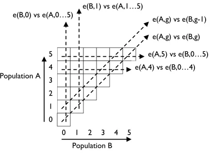
score-vectors of diminishing length. To visualise the values in this sequence of

vectors, fill the square cells in a triangular grid such as that shown in Figure 1with

gray-scales or colors that vary in accordance with the scalar values. For example,

normalise over all scores and then shade the highest-scoring cell black, the

lowest-scoring cell white, and assign appropriate shades of gray to cells with intermediate

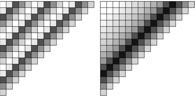
scores. Co-evolutionary dynamics such as limited evolutionary memory, or

intransitive dominance cycling, will then be revealed as certain qualitative visual

patterns, idealizations of which are shown in Figure 2. These could in principle be

detected by performing simple image processing on the CIAO plots. CIAO plots of

real data, such as that shown in Figure 3, tend to be more noisy and harder to

interpret than the idealizations of Figure 2.

Defined this way, CIAO plots are manifestly useful in generational co-evolutionary

systems where individuals compete one-on-one and are rated using an extrinsic

fitness evaluation function, but the visualisation technique would need to be

modified if it is to be applied to less explicitly sequenced systems, such as

steady-state systems; or to systems where the fitness function is implicit or intrinsic. Note

also that the computational cost of calculating the data for a CIAO plot rises as

O(½·G2_{) and so can easily become greater than the actual computational cost of the}

co-evolutionary experiment that the plot is generated to visualise.

* * * FIGURE 2 NEAR HERE * * *

* * * FIGURE 3 NEAR HERE * * *

3. Goodbye to all that?

We are of course pleased that other authors whose work we respect have

approvingly used the CIAO plot technique that we introduced, as it demonstrates

that our intuition regarding the need for such visualization tools was correct.

Nevertheless, we are even more pleased that Cartlidge & Bullock [1] have conducted

a careful dissection of the limitations of our method. Although CIAO plots have been

used by several authors over the years, the paper by Cartlidge & Bullock is the first

detailed exploration of the strengths and weaknesses of this visualization technique.

The central motivation for Cartlidge & Bullock’s paper is the observation that no CIAO plots of real experimental data have ever been published that resemble the

idealised plots of Figure 2. Instead, they note, almost all CIAO plots of real data are

much more reminiscent of ”banded” tartan or plaid patterns familiar from woven

textiles, and they explore why these tartan patterns occur, and what these patterns

might reveal about the underlying co-evolutionary dynamics. In doing so, they

that prominent bands are only shown in the CIAO plot when there is periodic

cycling through set of strategies, whereas aperiodic trajectories through strategy

space may not be readily identified from a CIAO plot.

Progress in any field is rarely if ever monotonic: the clear challenge now is to

develop visualization techniques better able to reveal qualitative, or even

References

[1] Cartlidge, J. & Bullock, S., (2004). Unpicking Tartan CIAO Plots: Understanding

irregular co-evolutionary cycling. Adaptive Behavior 12:69-92, 2004.

[2] Cliff, D. & Miller, G. F. (1995). Tracking the Red Queen: Measurements of

Adaptive Progress in Co-Evolutionary Simulations. In F. Morán, A. Moreno, J. J.

Merelo & P. Chacón (editors) Advances in Artificial Life: Proceedings of the Third European Conference on Artificial Life. Lecture Notes in Artificial Intelligence Vol. 929. Berlin: Springer-Verlag. pp.200-218.

[3] Floreano, D. & Nolfi, S. (1997). Adaptive behavior in competing co-evolving

species. In P. Husbands & I. Harvey (editors) Proceedings of the Fourth International Conference on Artificial Life. Cambridge MA: MIT Press. pp.378-387.

[4] Floreano, D. & Nolfi, S. (1997). God save the Red Queen! Competition in

co-evolutionary robotics. In J. R. Koza, K. Deb, M. Dorigo, D. B. Fogel, M. Garzon, H.

Iba, & R. L. Riolo (editors) Genetic Programming 1997: Proceedings of the Second Annual Conference. Morgan Kauffman. pp. 398-406.

[5] Ficici, S. G. & Pollack, J. B. (1998). Challenges in co-evolutionary learning:

H. Kitano, & C. Taylor (editors) Artificial Life VI. Cambridge MA: MIT Press. pp.238-247.

[6] Izuka, H. & Ikegami, T. (2004). Adaptability and Diversity in Simulated

Turn-Taking Behavior. Artificial Life, 10: 361-378. MIT Press.

[7] Nolfi, S. & Floreano, D. (1998). How co-evolution can enhance the adaptive power

of artificial evolution: Implications for evolutionary robotics. In P. Husbands & J.-A.

Meyer (editors) Evolutionary Robotics: First European Workshop (EvoRobot98). Lecture Notes in Computer Science Vol. 1468. Berlin: Springer-Verlag. pp.22-38.

[8] Rosin, C. D. & Belew, R. K. (1997). New methods for competitive co-evolution.

e(A,g) vs e(B,g-1)

e(B,0) vs e(A,0…5)

e(A,g) vs e(B,g)

e(A,5) vs e(B,0…5)

e(A,4) vs e(B,0…4)

Population A

0

1

2

3

4

5

5

4

3

2

0 1

Population B

e(B,1) vs e(A,1…5)

Figure 1. Schematic for constructing a CIAO plot for Population A. The square cells

would be shaded or colored to represent scores in competitions, the dashed lines

indicate different vectors of scores that could be visualized as conventional

Figure 2: Idealised CIAO plot patterns, with darker shading indicating higher scores.

Left: intransitive dominance cycling, where current elites score highly against

opponents from 3, 8, and 13 generations ago but not so well against generations

inbetween;. Right: limited evolutionary memory where the current elites do well

against opponents from three, four, and five generations ago, but much less well