Assessing the Measurement of Policy
Positions in Expert Surveys
Ren´
e Lindst¨
adt, Sven-Oliver Proksch & Jonathan B. Slapin
∗February 25, 2015
Paper prepared for the Biannual Meeting of the European Studies Association, Boston, MA, March 5th-7th, 2015.
Abstract
Expert surveys provide a common means for assessing parties’ policy positions on latent dimensions. These surveys often cover a wide variety of parties and issues, and it is unlikely that experts are able to assess all parties equally well across all issues. While the existing literature using expert surveys acknowledges this fact, insufficient attention has been paid to the variance in the quality of measurement across issues and parties. In this paper, we first discuss the nature of the measurement problem with respect to expert surveys and then propose methods borrowed from the organizational psychology and medical fields to assess the ability of experts to assess where parties stand on particular dimensions. While we apply our technique to one particular study, the Chapel Hill Expert Survey, the method can be applied to any expert survey. Finally, we propose a simple non-parametric bootstrapping procedure that allows researchers to assess the effects of expert survey measurement error in analyses that use them.
∗Ren´e Lindst¨adt is Professor of Government at the University of Essex, Sven-Oliver
1
Introduction
Expert surveys provide a common means of assessing the positions of political actors, most
notably parties, on a wide array of latent policy dimensions. Rather than estimate positions
directly from the actions that parties and their members take — e.g., votes or speeches —
researchers ask experts to synthesize their knowledge of a party system and assign positions
to parties on specific dimensions of interest. Depending upon the specificity of the dimensions
under investigation in the survey, researchers may require a great deal of detailed knowledge
from their experts. It is unlikely that experts are able to assess all parties equally well
across all dimensions, meaning that almost certainly some parties and some issues are better
measured than others. The existing expert survey literature in political science has explored
covariates to explain the variation in expert placement within parties, but we argue that this
approach is insufficient to understand the nature of the measurement problem in these data.
In this paper, we use techniques commonly found in the psychometric and medical fields
— intraclass correlation and within-group agreement — to assess levels of agreement and
reliability among experts when they place parties on scales in expert surveys. These
tech-niques allow us to examine agreement at the party-dimension level and account for the fact
that experts may use the scale in a different manner. To date political scientists conducting
and using expert surveys have given insufficient attention to the distinction between
inter-rater agreement and reliability and do not sufficiently examine the variability in quality of
responses of experts across parties and dimensions.
The paper proceeds by first discussing the nature of the measurement problem and
sta-tistical inference with respect to expert surveys. We then discuss the differences between
agreement and reliability, and introduce measures to capture each concept. To demonstrate
the extent of the measurement problem in expert surveys, we apply the measures to one
particular survey, the Chapel Hill Expert Survey (CHES). Lastly, we propose a simple
non-parametric bootstrapping procedure that allows researchers to assess the effects of expert
using the CHES data, we demonstrate that measurement error in expert surveys may have
consequences for our analyses.
2
Expert Surveys and Statistical Inference
As others have noted before (see Benoit and Laver, 2006, ch. 4), the statistical inference
problem in expert surveys differs quite substantially from that in public opinion surveys.
In public opinion surveys, researchers wish to measure a quantity of interest regarding a
population by randomly sampling observations from that population. For example, we draw
a random sample of voters from the population of all voters to assess the public’s support
for the US President. Opinion surveys ask n respondents to report their own opinions, xi,
to estimate a sample mean, ¯x, in an effort to make inferences about a population parameter,
µ, namely the true public support for the President. We consider each individual response,
xi, as a random draw from the true population distribution of support for the President. By
itself, each individual xi offers no useful information about µ. But according to the central
limit theorem, our estimate of µ, the true mean opinion of the President in the population,
improves as n increases.
Now compare this with the measurement problem when evaluating expert surveys. The
primary objective of expert surveys is to aggregate knowledge about states or political parties
or some other object of interest. Experts are not chosen at random from a population because
researchers are usually not interested in inferring the value of a parameter from a population
of experts. Rather, they are interested in gleaning information from them about a topic on
which they have expertise — in other words, the latent concept they wish to measure. In this
case, one highly knowledgeable expert may, in fact, be better than several lesser informed
ones. The problem, though, is that the researchers conducting the survey do not necessarily
know how knowledgeable their experts are. Assume that a party has a true, latent position
perfectly informed, they will all respond in an identical manner — that the party has a
position γ. Having one expert is as good as having 20. However, if the experts are not all
equally informed, or they are uniformly poorly informed, they may not all answer in the
same manner. Instead, each expert i may state that the party’s position is γ+i, where i
is drawn from some distribution D with mean, µ, and standard deviation σ. We might say
that γ is well-measured when D follows a symmetric distribution, µ=γ and σ is small. In
other words, all experts assign the party similar scores, which are tightly clustered around
the true score. As Dbecomes skewed,µdeviates from γ, andσ grows large, the experts are
less able to capture the position of the party or the nature of the dimension.
Interestingly, increasing the number of experts does nothing to improve the measurement
of γ. Benoit and Laver (2006, ch. 4) claim otherwise, saying that increasing the number of
experts increases the certainty around the estimate of the party position. They calculate
standard errors for party positions based on the standard deviation of expert placements as
well as the number of expert placements. However, this approach has almost unanimously
been rejected by the literature on interrater agreement (e.g., Kozlowski and Hattrup, 1992;
LeBreton and Senter, 2008). If experts were drawn at random from the population of all
experts, increasing respondents would shrink the standard deviation of the sampling
distri-bution of the mean expert perception of a party’s position. But being increasingly confident
about themean expert perception does not imply that experts are actually good at assessing
the latent party position. The sample distribution of expert placements could be uniformly
distributed across the entire range of the scale, yet with a sufficient number of experts, the
standard error of the mean would be quite small. Again, we are not interested in inference
about a population of experts, but rather we wish to learn about a latent characteristic of the
parties the experts are rating. Thus, the sampling distribution of the average expert opinion
is not of primary interest to us. Unlike with traditional statistical inference as applied to
opinion polls, when assessing the effectiveness of experts at capturing a latent position, it
responses does not provide us with a better measure of γ, but does allow us to get a better
sense of the shape of the distribution D.
However, to date none of the robustness and validity checks that political scientists
apply to expert survey responses adequately assess the shape of the distribution of expert
placements. Most analyses focus on the mean expert placement or, at best, the standard
deviation of placements (Hooghe et al., 2010).1 But in actuality, we are most interested in
the consistency and agreement of expert responses.2 In the remainder of the paper, we first demonstrate why the dominant approach in political science for assessing expert surveys is
problematic, and then propose a set of solutions and good practices.
3
Distribution of Expert Placements
We begin by demonstrating that the shape of expert placement distributions can vary quite
drastically. We examine policy dimensions from the commonly used Chapel Hill Expert
Survey (Bakker et al., forthcoming). The most recent iteration of the Chapel Hill survey,
conducted in 2010, queried 343 experts to estimate positions for 237 parties across 24 EU
member states on numerous dimensions. On average, slightly more than 13 experts
re-sponded per party-dimension. Expert surveys typically report the average expert placement
on each policy dimension in the published data (Benoit and Laver, 2006; Bakker et al.,
forthcoming). In practice, this can mean that political parties have an estimated mean
party position based on very different distribution of expert placements. We focus here on
five prominent dimensions from the Chapel Hill expert survey: three dimensions related
to the European Union (intra-party dissent on EU, the party position on the EU, and the
salience of the EU) and two dimensions related to the traditional left-right partisan
con-1Or in the case of Benoit and Laver (2006) the standard error.
2van der Eijk (2001) makes a similar point, but he focuses solely on agreement and fails
flict (left-right position on economic policy and general left-right position). Figure 1 shows
distributions of expert responses for six parties across the three EU dimensions. For each
dimension, we selected two parties with similar mean positions but different distributions of
expert responses. For instance, on the dimension measuring intra-party dissent, the mean
expert placement suggests that the Irish Fine Gael and the Greek New Democracy party
have moderate levels of intra-party dissent, denoted by the black vertical line. However,
whereas experts in Greece strongly disagree about the levels of intra-party dissent, leading
to a nearly bimodal distribution spanning the entire scale, experts in Ireland agree that Fine
Gael only has moderate levels of dissent. Figure 1 includes similar graphs for the Dutch
VVD and Finnish SDP on the EU dimension and for the Hungarian JOBBIK and French
Greens on the EU salience dimension. In each case, experts cannot agree on the placement
of one party. And in two of the three instances, the party was a mainstream and not a fringe
party.
Similarly, the left-right dimension, which typically shows smaller variation in expert
placements, is subject to the same problems. Figure 2 presents expert placements for
left-right economic policy for the French Front National and the Polish Civic Platform. For the
Front National, we observe a distribution of expert placements that is bimodal. On average,
the Front National is estimated to be a centre-right party, but the contrast to the Civic
Platform in Poland — a party with a similar average position — is obvious. Experts use
almost the entire scale to place the French party, whereas there is agreement among experts
that the Polish party is centre-right. This contrast occurs even on the (supposedly best)
measured dimension, the general left-right dimension. Here, experts have trouble locating the
DeSUS from Slovenia, whereas they agree strongly on the Portuguese PS. In the aggregate,
however, both parties are estimated to hold identical left-right positions. These illustrations
New Democracy (Greece)
EU Dissent Expert Placements
Frequency
0 2 4 6 8 10
0.0
0.5
1.0
1.5
2.0
2.5
3.0
Fine Gael (Ireland)
EU Dissent Expert Placements
Frequency
0 2 4 6 8 10
0
1
2
3
4
(a) EU Dissent
VVD (Netherlands)
EU Position Expert Placements
Frequency
0 2 4 6 8 10
0
1
2
3
4
5
6
Social Democratic Party (Finald)
EU Position Expert Placements
Frequency
0 2 4 6 8 10
0
1
2
3
4
5
6
(b) EU Position
JOBBIK (Hungary)
EU Salience Expert Placements
Frequency
0 1 2 3 4
0
1
2
3
4
5
VERTS (France)
EU Salience Expert Placements
Frequency
0 1 2 3 4
0
2
4
6
8
[image:7.612.119.484.78.694.2](c) EU Salience
Front National (France)
LR Econ Expert Placements
Frequency
0 2 4 6 8 10
0.0
0.5
1.0
1.5
2.0
2.5
3.0
Civic Platform (Poland)
LR Eon Expert Placements
Frequency
0 2 4 6 8 10
0
1
2
3
4
5
6
7
(a) Left/Right Economic Policy
DeSUS (Slovenia)
LR Expert Placements
Frequency
0 2 4 6 8 10
0
1
2
3
4
5
PS (Portugal)
LR Expert Placements
Frequency
0 2 4 6 8 10
0.0
0.5
1.0
1.5
2.0
2.5
3.0
[image:8.612.115.482.153.592.2](b) Left/Right General
4
Measures of Agreement and Reliability
The political science literature has largely confined itself to looking at expert placement
means, standard deviations, and standard errors.3 Beyond political science, though, a large
literature in (organizational) psychology and medicine seeks to understand how to best assess
agreement and reliability in responses to particular (survey) items. The same issues that
crop up in political science expert surveys arise in any analysis in which K raters score N
targets on J items. In medicine, multiple doctors may rate patients on several scales to
arrive at a diagnosis. In organizational psychology, researchers often ask employees at a firm
about their perceptions of various items, such as the firm’s adequacy in handling consumer
complaints, on a Likert scale. In these examples, the doctors and employees are equivalent
to our experts, the patients and firm equivalent to our parties, and the various scales, to our
dimensions.
The literature makes a significant distinction between reliability and agreement.
Ko-zlowski and Hattrup (1992, pp. 162–63) describe reliability “as an index of consistency; it
references proportional consistency of variance among raters [. . . ] and is correlational in
na-ture [. . . ]. In contrast, agreement references the interchangeability among raters; it addresses
the extent to which raters make essentially the same ratings.” In other words, reliability
is concerned with the equivalence of relative ratings of experts across items, whereas
agree-ment refers to the absolute consensus among raters on one or more items (LeBreton and
Senter, 2008, p. 816). Thus, there could be relatively high reliability among raters, but low
agreement. For example, all raters may rate party A higher than party B than party C, but
they may use the scale differently. On an eleven point 0–10 left-right scale, perhaps Rater 1
assigns a 10, 8, and 6 to parties A, B and C respectively; Rater 2 assigns them scores of 8,
6, and 4; and Rater 3 rates them 4, 2, and 0. There would be perfect reliability among these
scores, but little agreement. It is worth noting that reliability can only be assessed when the
3One exception is van der Eijk (2001), who constructs an agreement index, which we will
same raters rate multiple targets (e.g., parties), and thus can only be assessed at the item
level. Agreement, in contrast, can be assessed at the target-item level.
We discussed above that the literature on interrater agreement has deemed the standard
error to be an inappropriate measure of agreement, but it also suggests that the standard
deviation is not much better. The standard deviation is a measure of dispersion, rather than
agreement. There are two primary drawbacks to the standard deviation as a measure of
agreement (Kozlowski and Hattrup, 1992). First, the standard deviation is scale-dependent
— items assessed on a Likert scale ranging from 0–10 will likely have a smaller standard
deviation than those assessed on a 0–100 scale — such that we can only compare standard
deviations of items that are measured on the same scale. Second, it does not account for
within-group agreement that could occur due to chance. The most common measure of
agreement, the rwg (Finn, 1970; James, Demaree and Wolf, 1984), does both by examining
the dispersion of responses with reference to a null distribution. It is calculated as
rwg = 1−
S2
x
σ2
E
, (1)
where S2
x is the observed variance of expert response on the itemx, and σE2 is the expected
variance when there is a complete lack of agreement among experts.4 The measure ranges
from 0 (no agreement) to 1 (perfect agreement) and can be interpreted as the proportional
reduction in error variance.5 Of course, r
wg requires researchers to choose an appropriate
null distribution. In practice, researchers typically use a rectangular or uniform distribution,
estimated as A212−1, where A is the number of response options. But any number of
distri-4One could also calculate agreement across multiple items, using the r
wg(j) measure, if
the items were essentially parallel, meaning that they measure the same construct. Given that most items in political science surveys tap into different dimensions, this measure is less appropriate for our purposes.
5In rare instances, it could be negative, meaning there is more observed variance than we
butions could be used, and ideally one’s results would be robust to the choice of the null
distribution (Meyer et al., 2014). At the moment, we use the rectangular distribution as the
null distribution.
The rwg measure captures agreement, but does not take into account differences in how
raters may use the scale. For that, we need a measure of reliability, which examines how
judges place multiple targets. Here we use a measure of intraclass correlation. In
partic-ular, we employ a two-way mixed-effects intraclass correlation coefficient. This measure is
appropriate when a fixed set of K judges assesses multiple targets on multiple items. It is
calculated as follows
ICC = M SR−M SE
M SR+ (K −1)M SE +KN(M SC−M SE)
, (2)
where M SR is the mean square of the targets, M SC is the mean square for the judges, and
M SE is the mean square error (LeBreton and Senter, 2008). This measure captures both
the consensus among as well as the consistency across judges. In effect, if we knew that
judges used the scales in the same manner, we could arrive at the same answer by simply
aggregating the rwg scores over the targets on each item.
5
Application to the Chapel Hill Expert Survey
We now apply these measures of agreement and reliability to the 2010 CHES expert survey
discussed above. We first calculate the rwg measure, which captures agreement only. The
advantage of the rwg coefficient is that, since we are only concerned with agreement and not
reliability, it can be applied to the party-dimension level. The disadvantage, of course, is that
it cannot account for differences in how experts use the scale (i.e., reliability). We use box
plots to display the distribution ofrwg coefficients by dimension across parties and by party
across dimensions. These plots are displayed in Figures 3 and 4. There are no hard and fast
considers scores in excess of 0.7 to be indicative of strong agreement and scores below 0.5 of
weak agreement. In Figures 3 and 4, these two cut-off values are demarcated with vertical
dashed lines.
The first plot, Figure 3a, displays a box plot for each party in the CHES data. Due to
the large number of parties, it is difficult to assess how any particular party is measured.
Thus, we suppress the party names on the y-axis and do not plot outlying points in this
figure. The purpose of the plot is not to see where individual parties lie, but rather to show
the overall distribution of the levels of agreement across all parties. The plot does show that
there are many parties for which the median rwg over the dimensions is quite a bit better
than the 0.7 cut-off for strong agreement. It is also worth noting that even for the parties
on which experts agree quite often, there are many dimensions with agreement scores in the
moderate or even poor range. There are also many party-dimensions for which there is only
moderate or poor agreement. Figure 3b presents box plots by dimension. Again, we see that
there is particularly low agreement on the salience items. Figure 4 plots the best performing
parties (i.e., those with a median dimension rwg > 0.75) and the worst performing parties
(i.e., those with a median rwg <0.55).
Most of the parties with the highest levels of agreement are found in northern and western
Europe. However, some parties in post-communist countries also show high levels of
agree-ment, namely some Latvian, Czech, and Slovenian parties. The parties with the lowest levels
of agreement among experts are found in southern and eastern Europe. There is virtually no
agreement on the positions of the Turkish parties on many dimensions. But even here, there
is strong agreement on certain items for certain parties. For example, on the CHES
gal-tan dimension (Green/Alternative/Libertarian to Traditional/Authoritarian/Nationalist),
the ruling AK party, the MHP, the DYP and the Greens all display high agreement, while
the CHP and BDP display virtually no agreement at all. Thus, while there appears to be
agreement with respect to the center-right Islamist parties AKP and DYP, the
for much of the post-war era, or the Kurdish BDP. Interestingly, while in most countries
the left-right general and left-right economics dimensions display more agreement than the
galtan dimension, in Turkey, with the exception of the AKP, experts display higher levels of
agreement on the galtan dimension than on either of the left-right dimensions.
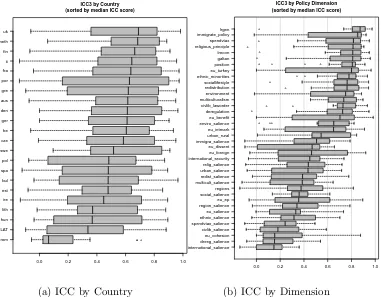
We next calculate the intraclass correlation coefficient (ICC), which accounts for both
agreement and reliability (i.e., scale shifts across experts). As discussed above, we use a
two-way mixed-effects ICC. Because we assess expert placements across parties, the coefficients
are measured at the level of country-dimension. We again plot the results in two different
ways. Using box plots, we first examine the distribution of ICC coefficients within country
and across dimensions (Figure 5a) and then within dimension across countries (Figure 5b).
The distributions of ICC coefficients reveal interesting trends, similar to those found
using the agreement scores. ICC is higher in virtually every EU15 state compared with
new members from Eastern Europe, with particularly low ICCs in Romania. With respect
to dimension, Left-Right General is the best-measured dimension based on ICC. Other
di-mensions, including immigration policy, taxes vs. spending, religious principles, left-right
economics, galtan, andEU position, perform also quite well. There is less agreement among and reliability across experts when considering salience items and items, such as intra-party
dissent on EU integration. It should be noted, though, that parties with missing data on
any dimension are not included in the analysis. On average, 3.66 fewer parties per
country-dimension are included in our analysis than are scored in the original data. In future work,
we will examine various methods to handle missing data. If anything, dropping these parties
biases our results towards finding more agreement and reliability than actually exists, since
6
Including Uncertainty in Secondary Analysis via the
Bootstrap
The Rwg and ICC coefficients provide a useful means to assess the extent of measurement
error in expert surveys across different parties and policy dimensions. Once we know that a
lack of agreement among experts exists, we would ideally take this information into account
when building empirical models. However, researchers do not incorporate the information
contained in these coefficients into analyses in a straightforward manner. Existing approaches
to handling measurement error require finding an appropriate instrument for the poorly
measured variable (Hausman, 2001), or using an estimate of the measurement error in a
simulation-extrapolation (SIMEX) model (Cook and Stefanski, 1994). In the case of expert
positions, we often have neither of these. Matters are complicated if the quantity of interest
in the secondary analysis relies on a transformation of party positions, such as party system
polarization or shifts in party positions between elections. Because not all parties are equally
well measured, we do not knowa priori how variation across expert placements affects such
derived measures.
To account for uncertainty around expert placements of parties, we propose a simple
solution: bootstrapping observed expert responses by sampling with replacement from the
observed expert responses. Through a non-parametric bootstrap we can generate n expert
datasets and calculate any quantity of interest within them (e.g. mean expert placements,
party system polarization, etc.). Any regression analysis using expert placements, or a
derivation thereof, as an independent variable can then be conducted n times using the
simulated values of the expert placements. The coefficients and their associated uncertainty
estimates across these n models can then be averaged just as one would do with multiply
imputed datasets when faced missing data. Indeed, missing data can be thought of as a
special case of measurement error (Blackwell, Honaker and King, 2014). This approach is
the measurement error associated with a variable measured using a Bayesian measurement
model.
Party System Polarization
Measuring party system polarization has a long tradition in the comparative literature on
party politics (e.g. Taylor and Herman, 1971; Gross and Sigelman, 1984; Alvarez and Nagler,
2004; Sartori, 2005; Dalton, 2008; Rehm and Reilly, 2010). In their study on the effects of
elite communication over European integration on public opinion, Gabel and Scheve (2007)
rely on expert surveys to calculate polarization measures for several European countries.
Following Warwick (1994), they calculate the weighted standard deviation of party positions
in each countryk as follows:
Polarizationk=
v u u t
N
X
j=1
vj(xjk−x¯k)2,
wherevj is the j-th party’s share of the vote in countryk with N parties (excluding parties
who do not receive any votes),xjk is the placement of thej-th party on European integration
by the experts, and ¯xk is the weighed mean of parties on European integration, where each
party is weighted by its vote share.6 Gabel and Scheve calculate these measures using data
from the Chapel Hill expert survey (Steenbergen and Marks, 2007).
We replicate the polarization measures for the 1999 Chapel Hill survey and generate
confidence intervals for them using 100 bootstrapped expert datasets. The average
boot-strapped polarization measure correlates with their original measure at 0.97. Figure 6 shows
the bootstrapped mean estimates and the confidence intervals, which correspond to the
2.5-th and 97.5-2.5-th percentile of 2.5-the bootstrapped polarization measure. When we take into
account the uncertainty in expert placements, there are a number of countries for which we
6The equation in footnote 4 in their paper erroneously mentions the mean instead of the
cannot safely conclude that their polarization measures are different from each other. For
instance, Belgium is estimated to have a mean polarization measure that is forty percent
greaterthan Spain’s. However, on the basis of the variability of expert placements for some of the parties, we actually cannot reject the null hypothesis that the two measures are identical.
Not all countries are equally affected by measurement error. For instance, elite polarization
on European integration is well measured in Denmark, Germany, and Greece, but poorly
measured in countries such as Finland, Spain, and United Kingdom. In sum, these results
demonstrate that a simple incorporation of the measurement uncertainty can translate into
sizable measurement error in a derived variable such as party system polarization.
Party Position Shifts
The Chapel Hill surveys have also recently been used to answer questions about
mass-elite linkages. Here, we look at one particular study from this literature by Adams, Ezrow
and Somer-Topcu (2014), who propose an innovative research design to improve our
under-standing of how citizens update their views on parties’ policy positions. Specifically, their
argument states that citizens, rather than relying on party manifestos to update their
in-formation on party policy positions — a view that has had a long tradition in the extant
literature —, draw on a variety of information sources when updating their beliefs.
Clearly, testing this proposition using standard mass survey instruments would be quite
difficult (though, probably not impossible), which is why Adams, Ezrow and Somer-Topcu
use expert opinions from the Chapel Hill surveys as a proxy for broad information gathering
and contrast it with the more narrow approach of relying on party manifestos. In particular,
they hypothesize that if mass public opinion on party policy shifts more closely tracks expert
opinions on these shifts than policy shifts derived from party manifestos, then this suggests
that citizens rely on multiple information sources. Their empirical analysis confirms the
hypothesis, and the finding is an important contribution to the ongoing debate about political
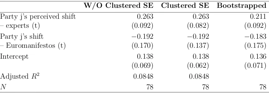
Table 1: Analyses of Citizens’ Perceptions of Parties’ Policy Shifts on European Integration (Adams, Ezrow and Somer-Topcu, 2014).
W/O Clustered SE Clustered SE Bootstrapped
Party j’s perceived shift 0.263 0.263 0.211
– experts (t) (0.092) (0.082) (0.092)
Party j’s shift −0.192 −0.192 −0.183
– Euromanifestos (t) (0.170) (0.137) (0.175)
Intercept 0.138 0.138 0.136
(0.069) (0.062) (0.071)
Adjusted R2 0.0848 0.0848
N 78 78 78
Of course, the concern is that measurement error resulting from aggregating potentially
divergent expert opinions on party policy shifts drives these results. To address this question,
we applied the same bootstrap method described above to Adams, Ezrow and Somer-Topcu
analysis. We present the results of our empirical analysis in Table 1.
Specifically, we estimate three different models. The first model in Table 1 replicates
theMultivariate Model (3) in Adams, Ezrow and Somer-Topcu, but without clustering. The second model in Table 1 uses clustered standard errors and therefore is an exact replication of
theirMultivariate Model (3). Comparing the results from these two regressions clearly shows
that the clustering has very little effect on the standard errors, and the substantive results
do not change across these two regressions (i.e., no changes in statistical significance). As
such, we proceed to estimate the third model in Table 1, which summarizes the coefficients
and standard errors from 100 bootstrap regressions, without clustering.
The first thing to notice in Table 1 is that the results are remarkably robust, giving
additional credence to the findings by Adams, Ezrow and Somer-Topcu. Yet, taking a closer
look at the bootstrapped results also shows that the coefficient is smaller and standard
error estimates are larger than in the original regression. Stated differently, on average, our
substantive results do not change with this application, the increase in uncertainty around
the estimates should give us pause for using aggregate expert opinions in our regressions
without considering the level of disagreement among experts.
7
Conclusion
Political scientists make frequent use of expert surveys, but have not properly examined
agreement and reliability within these surveys. A vast literature in organizational psychology
and medicine provides us with the tools to assess the degree to which experts can capture the
latent dimensions of party politics that are of interest to political scientists. In this paper,
we have applied these techniques to one particularly prominent expert survey. The methods,
though, are very general and can be applied in any number of settings. The analysis has
clearly uncovered that the positions of some parties and on some dimensions are clearly easier
to assess than others. General items, such as left-right general, left-right economic policy, and
position with respect to EU integration, are clearly easier to capture than more specific items.
In addition, positions are clearly easier to gauge than saliency. Lastly, experts in advanced
industrialized countries are better able to capture parties in their countries compared with
experts from newer, post-communist democracies. Because experts only rank parties in one
country — the country where they have the greatest expertise — we cannot say whether
this is a function of the experts, the parties they are asked to rate, or both.
In future iterations, we plan to examine the effect of relaxing the assumption about the
null distribution. Lastly, we will account for missing data in the bootstrap procedure. In
doing so, we will be able to make recommendations to researchers looking to conduct expert
surveys with regard to how many experts they should ask and what type of items are most
0.0 0.2 0.4 0.6 0.8 1.0
Agreement Score Rwg (sor
ted b y median) (a) Rw g b y P art y ● ● ● ●● ● ● ●● ● ● ● ●● ●● ● ● ● ● ● ●● ● ● ● ● ● ●● ● ● ● ●● ● ● ●● ●● ● ● ●● ● ●●●●●●●●●●●●● ● ●● ● ●●●●●●● ● ●● ● ●●●●●●●● ● ●●●● ● ●● ●● ● ●● ● ● ● ● ●● ● ● ● ● ● ● ●● ● ● ● ● ●●●● ● ● ● ● ● ● ● ● ● ● ● ● ● ● ● ● ● ● ● ● ● ● ● ●●● ● ● ●● ● ●● ● ● ● ● ● ● ● ●● ● ● ●● ● ● ●●●● ● ●● ● ● ● ●●●●●● ●●●●●●● ● ● ●● ● ● ●●● ● ● ● ● ● ● ● ● ●● ● ● ● ● ● ● ● ● ●● ● ● ● ● ● ●● ● ● ● ● ● ● ● ● ● ● ● ●● ● ● ● ● ● ● ● ● ● ● ● ● ● ● ● ● ● ● ● ● ● ● ● region_salience inter national_salience relig_salience ethnic_salience social_salience dereg_salience urban_salience immigr a_salience m ulticult_salience spendvtax_salience civlib_salience redist_salience inter national_secur ity eu_salience eu_dissent en viro_salience regions eu_f oreign eu_intmar k religious_pr inciple eu_ep ethnic_minor ities sociallif estyle m ulticultur alism en vironment civlib_la w order eu_tur k e y urban_r ur al deregulation galtan immigr ate_policy eu_cohesion spendvtax redistr ib ution eu_position lrecon lrgen 0.0 0.2 0.4 0.6 0.8 1.0
Agreement Score Rwg
● ● ● ● ● ● ● ● ● ● ● ● ●● ● ● ● ●● ● ● ● ●● ● ● ● ● ● ● ● ● ● ●● ● ● ● ● ● ●● ● ● ● ● ●● ● ● ● ● ● ● ● ● ● ● ● ● ● ● ● ● ● ● ● ● swi:LdT swi:GPS/PES swi:EVP/PEV slo:LS−HZDS nor:Sp spa:CC slo:KDH cze:KDU−CSL ger:SPD aus:SPO gre:OP den:SD uk:LAB slo:SF den:V swe:C swi:SPS/PSS por:PSD den:KF ger:CSU neth:CU LAT:V den:RV fin:SFP nor:SV swi:CVP/PVC spa:EdP−V it:PSI uk:GREEN fin:VAS nor:DNA nor:H uk:LIB fin:KESK nor:KrF LAT:NA neth:CDA swe:V fin:VIHR ger:CDU aus:OVP fin:KOK spa:CpE fin:SDP
0.0 0.2 0.4 0.6 0.8 1.0
Agreement Score Rwg (sorted by median)
(a) MedianRwg >0.75
tur:AKP bul:L bul:RZS tur:CHP tur:BDP lith:FRONT rom:PRM pol:S cro:HDSSB cro:HSP hun:JOBBIK gre:KKE hun:LMP it:MpA bul:DSB be:LDD fra:FN ger:LINKE ire:SF bul:NOA ire:SP pol:LPR lith:TT neth:PVV sle:SDS be:PVDA rom:PNL bul:BNS tur:GP lith:TS rom:PC tur:MHP sle:NSI rom:UDMR cze:KSCM it:AN
0.0 0.2 0.4 0.6 0.8 1.0
Agreement Score Rwg (sorted by median)
[image:20.612.123.508.240.532.2](b) Median Rwg <0.55
● ● ● rom LAT hun lith ire est bul spa pol swe cze be ger den aus gre por fra it fin neth uk
0.0 0.2 0.4 0.6 0.8 1.0 ICC3 by Country
(sorted by median ICC score)
(a) ICC by Country
●● ● ● ● ● ● ● ● ● ● ● ● ● ● ● ● ● ● international_salience dereg_salience eu_cohesion civlib_salience spendvtax_salience ethnic_salience eu_salience region_salience eu_ep social_salience regions multicult_salience redist_salience urban_salience relig_salience international_security eu_foreign eu_dissent immigra_salience urban_rural eu_intmark enviro_salience eu_benefit deregulation civlib_laworder multiculturalism environment redistribution sociallifestyle ethnic_minorities eu_turkey position galtan lrecon religious_principle spendvtax immigrate_policy lrgen
0.0 0.2 0.4 0.6 0.8 1.0 ICC3 by Policy Dimension
(sorted by median ICC score)
[image:21.612.125.506.236.533.2](b) ICC by Dimension
Polarization Measure and 95% Confidence Intervals
Ireland Spain Netherlands Germany Italy Finland Belgium Portugal Greece Sweden United Kingdom Austria Denmark France
1.0 1.5 2.0
● ●
● ●
● ●
● ●
● ●
● ●
[image:22.612.91.528.221.547.2]● ●
References
Adams, James, Lawrence Ezrow and Zeynep Somer-Topcu. 2014. “Do Voters Respond to Party Manifestos or to a Wider Information Environment? An Analysis of Mass-Elite
Linkages on European Integration.”American Journal of Political Science .
Alvarez, R.M. and J. Nagler. 2004. “Party System Compactness: Measurement and
Conse-quences.”Political Analysis 12(1):46–62.
Bakker, Ryan, Catherine de Vries, Erica Edwards, Liesbet Hoogh, Seth Jolly, Gary Marks, Jonathan Polk, Jan Rovny, Marco Steenbergen and Milada Anna Vachudova. forthcoming. “Measuring Party Positions in Europe: The Chapel Hill Expert Survey Trend File,
1999-2010.”Party Politics .
Benoit, Kenneth and Michael Laver. 2006. Party Policy in Modern Democracies. Routledge.
Blackwell, Matthew, James Honaker and Gary King. 2014. “A Unified Approach to Mea-surement Error and Missing Data: Details and Extensions.” Working Paper.
Cook, J. and L. Stefanski. 1994. “Simulation-Extrapolation Estimation in Parametric
Mea-surement Error Models.” Journal of American Statistical Association 89(428):1314–1328.
Dalton, R.J. 2008. “The Quantity and the Quality of Party Systems.”Comparative Political
Studies41(7):899.
Finn, R.H. 1970. “A note on estimating the reliability of categorical data.”Educational and
Psychological Measurement30:71–76.
Gabel, Matthew and Kenneth Scheve. 2007. “Estimating the effect of elite communications
on public opinion using instrumental variables.” American Journal of Political Science
51(4):1013–1028.
Gross, D.A. and L. Sigelman. 1984. “Comparing Party Systems: A Multidimensional
Ap-proach.”Comparative Politics 16(4):463–479.
Hausman, Jerry. 2001. “Mismeasured Variables in Econometric Analysis: Problems from the
Right and Problems from the Left.” The Journal of Economic Perspectives 15(4):57–67.
Hooghe, Liesbet, Ryan Bakker, Anna Brigevich, Catherine De Vries, Erica Edwards, Gary Marks, Jan Rovny, Marco Steenbergen and Milada Vachudova. 2010. “Reliability and
Validity of the 2002 and 2006 Chapel Hill Expert Surveys on Party Positioning.”European
Journal of Political Research49(5):687–703.
James, Lawrence R., Robert G. Demaree and Gerrit Wolf. 1984. “Assessing within-group
interrater reliability with and without response bias.” Journal of Applied Psychology
69(1):85–98.
Kozlowski, Steve W.J. and Keith Hattrup. 1992. “A Disagreement About Within-Group
Agreement: Disentangling Issues of Consistency Versus Consensus.” Journal of Applied
LeBreton, James M. and Jenell L. Senter. 2008. “Answers to 20 Questions about Interrater
Reliability and Interrater Agreement.”Organizational Research Methods 11(4):815–852.
Meyer, Rustin D., Troy V. Mumford, Carla J. Burrus, Michael A. Campion and Lawrence R. James. 2014. “Selecting Null Distributions When Calculation Rwg: A Tutorial and
Re-view.” Organizational Research Methods DOI: 10.1177/1094428114526927.
Rehm, Philipp and Timothy Reilly. 2010. “United We Stand: Constituency Homogeneity
and Comparative Party Polarization.” Electoral Studies 29(1):40–53.
URL: http://dx.doi.org/10.1016/j.electstud.2009.05.005
Sartori, G. 2005. Parties and Party Systems: A Framework for Analysis. European
Consor-tium for Politcal Research.
Steenbergen, Marco R and Gary Marks. 2007. “Evaluating expert judgments.” European
Journal of Political Research46(3):347–366.
Taylor, M. and V.M. Herman. 1971. “Party Systems and Government Stability.” American
Political Science Review65(1):28–37.
Treier, Shawn and Simon Jackman. 2008. “Democracy as a Latent Variable.” American
Journal of Political Science52(1):201–217.
van der Eijk, Cees. 2001. “Measuring Agreement in Ordered Rating Scales.” Quality and
Quantity 35(3):325–341.
Warwick, Paul. 1994. Government survival in parliamentary democracies. Cambridge Univ