Adaptive Minimum Bit Error Rate Beamforming Assisted Receiver for QPSK Wireless Communication

Adaptive minimum bit error rate beamforming

assisted receiver for QPSK wireless communication

S. Chen

, L. Hanzo, N.N. Ahmad, A. Wolfgang

School of Electronics and Computer Science, University of Southampton, Southampton, SO17 1BJ, UK

Available online 25 March 2005

Abstract

This paper considers interference limited communication systems where the desired user and in-terfering users are symbol-synchronized. A novel adaptive beamforming technique is proposed for quadrature phase shift keying (QPSK) receiver based directly on minimizing the bit error rate. It is demonstrated that the proposed minimum bit error rate (MBER) approach utilizes the system re-source (antenna array elements) more intelligently, than the standard minimum mean square error (MMSE) approach. Consequently, an MBER beamforming assisted receiver is capable of providing significant performance gains in terms of a reduced bit error rate over an MMSE beamforming one. A block-data based adaptive implementation of the theoretical MBER beamforming solution is de-veloped based on the classical Parzen window estimate of probability density function. Furthermore, a sample-by-sample adaptive implementation is also considered, and a stochastic gradient algorithm, called the least bit error rate, is derived for the beamforming assisted QPSK receiver.

2005 Elsevier Inc. All rights reserved.

Keywords: Adaptive beamforming; Quadrature phase shift keying; Mean square error; Least mean square; Bit error rate; Probability density function; Parzen window estimate; Least bit error rate

* _{Corresponding author.}

E-mail addresses: [email protected] (S. Chen), [email protected] (L. Hanzo), [email protected] (N.N. Ahmad), [email protected] (A. Wolfgang).

1. Introduction

The ever-increasing demand for mobile communication capacity has motivated the de-velopment of adaptive antenna array assisted spatial processing techniques [1–12] in order to further improve the achievable spectral efficiency. A particular technique that has shown real promise in achieving substantial capacity enhancements is the use of adaptive beam-forming with antenna arrays. Through appropriately combining the signals received by the different elements of an antenna array to form a single output, adaptive beamforming is capable of separating signals transmitted on the same carrier frequency, provided that they are separated sufficiently in the spatial domain. Classically, this has been achieved by minimizing the mean square error (MSE) between the desired output and the actual array output, and this principle is rooted in the traditional beamforming employed in sonar and radar systems. Adaptive implementation of the theoretical minimum MSE (MMSE) beam-forming solution can readily be realized using temporal reference techniques [2–4,13–17]. Specifically, block-data based beamformer weight adaptation can be achieved using the so-called sample matrix inversion (SMI) algorithm [13,14], while sample-by-sample adap-tation can be carried out using the least mean square (LMS) algorithm [15–17].

For a communication system, it is the achievable bit error rate (BER), not the MSE performance, that really matters. Ideally, the system design should be based directly on minimizing the BER, rather than the MSE. For applications in single-user channel equal-ization and code division multiple access (CDMA) multiuser detection, it has been shown that the MMSE solution can in certain situations be distinctly inferior in comparison to the minimum BER (MBER) solution, and several adaptive implementations of the theoretical MBER solution have been studied in Refs. [18–22]. The recent conference paper [23] of the authors proposed an MBER beamforming assisted receiver for binary phase shift keying (BPSK) communication systems, where the desired user and interfering users are symbol-synchronized. This paper derives an adaptive beamforming technique based on directly minimizing the system’s BER for such interference limited systems employing quadrature phase shift keying (QPSK) modulation. It is demonstrated that the MBER solution utilizes the array weights more intelligently than the MMSE approach. The MBER beamforming appears to be “smarter” than the MMSE solution, since it directly optimizes the system’s BER performance, rather than minimizing the MSE, where the latter strategy often turns out to be deficient. In particular, when facing strong interfering sources, the MMSE beam-forming receiver may exhibit a high BER floor as the underlying signal classes become linearly inseparable, while the MBER beamforming receiver can often maintain the linear separability and hence avoids such a BER floor.

also been considered and an adaptive stochastic gradient MBER algorithm, referred to as the least bit error rate (LBER), is derived. This LBER algorithm has a low computational complexity which is comparable to that of the very simple LMS algorithm. Simulation results suggest that the LBER algorithm converges reasonably fast.

Before presenting our novel MBER QPSK beamforming technique, the assumption that the desired user and interfering signals are symbol-synchronized is elaborated on. For such a symbol-synchronized interference-limited QPSK system the non-Gaussian na-ture of the interfering signals is effectively exploited by the MBER beamforming receiver, resulting in an improved BER performance. For the downlink scenario synchronous trans-mission of the users is guaranteed. By contrast, in an uplink scenario the differently delayed asynchronous signals of the users are no longer automatically synchronized. However, the quasi-synchronous operation of the system may be achieved with the aid of adap-tive timing advance control, as in the global system of mobile communications, known as GSM [28]. The GSM system has a timing-advance control accuracy of 0.25 bit dura-tion. Since synchronous systems perform better than their asynchronous counterparts [29], the third-generation partnership research consortium known as 3GPP is also considering the employment of timing-advance control in next-generation systems. In general, when the number of users is large, the users are asynchronous and the idealistic assumption of perfect power control is stipulated, the performance gain of the (symbol-rate) MBER so-lution over the MMSE beamformer may be expected to diminish, since the interference becomes nearly Gaussian at the symbol-rate samples. One way of maintaining the benefits of the MBER solution for asynchronous systems is to perform a joint MBER detection and synchronization by sampling faster than the symbol rate. During each symbol period, sev-eral signal samples are taken and the receiver maintains sevsev-eral tentative MBER detectors. The detector having the smallest BER is chosen to perform symbol detection.

2. System model

It is assumed that the system supportsMsymbol-synchronized users, that is, there ex-istM synchronized signal sources, and each user transmits a QPSK modulated signal on the same carrier frequency ofω=2πf. The baseband complex-valued signal of useri, sampled at the symbol rate, is formulated as

mi(k)=Aibi(k), 1iM, (1)

wherebi(k)∈ {±1±j}are QPSK symbols, the complex-valuedAi is the channel

coef-ficient for useri multiplying by the transmitted signal amplitude of useri, and therefore 2|Ai|2denotes the received signal power of useri. Without any loss of generality, source 1

is assumed to be the desired user and the rest of the sources are the interfering users. The linear antenna array considered consists ofLuniformly spaced elements, and the signals received by theL-element antenna array are given by

xl(k)= M

i=1

mi(k)exp

j ωtl(θi)

wheretl(θi)is the relative time delay at array element l for sourcei,θi is the direction

of arrival for sourcei, and nl(k) is the complex-valued white Gaussian noise having a

zero mean and a variance ofE[|nl(k)|2] =2σn2. The desired user’s signal to noise ratio is

defined as SNR= |A1|2/σn2, the interference to noise ratio of interfering useriis given by

INRi= |Ai|2/σn2, the desired signal to interference ratio with respect to interfering useri

is defined as SIRi= |A1|2/|Ai|2, fori=2, . . . , M, and the desired signal to interference

plus noise ratio is given by SINR= |A1|2/(Mi=2|Ai|2+σn2). In a vector form, the array

input x(k)= [x1(k)x2(k) . . . xL(k)]T can be expressed as

x(k)= ¯x(k)+n(k)=Pb(k)+n(k), (3) where n(k)= [n1(k) n2(k) . . . nL(k)]T has a covariance matrix ofE[n(k)nH(k)] =2σn2IL

with ILrepresenting theL×Lidentity matrix, the system matrix P is given by

P= [A1s1A2s2. . . AMsM], (4)

the steering vector for sourceiis formulated as

si=

expj ωt1(θi)

expj ωt2(θi)

. . .expj ωtL(θi)

T

(5)

and the transmitted QPSK symbol vector is b(k)= [b1(k) b2(k) . . . bM(k)]T.

A standard linear beamformer is employed at the receiver, and the beamformer’s output is given by

y(k)=wHx(k)=wHx¯(k)+wHn(k)= ¯y(k)+e(k), (6)

where w= [w1w2. . . wL]T is the complex-valued beamformer weight vector, ande(k)is

Gaussian distributed having a zero mean and a variance ofE[|e(k)|2] =2σ_n2wHw. Define

the combined impulse response of the beamformer and the system as

wHP= [c1c2. . . cM]. (7)

The beamformer’s output can alternatively be expressed as

y(k)=c1b1(k)+

M

i=2

cibi(k)+e(k), (8)

where the first term is the desired signal and the second term the residual interference. Define the decision variable asd(k)=y(k)/c1. Then the decision regarding the transmitted

symbolb1(k)is made according to

ˆ

b1(k)=sgn

dR(k)

+jsgndI(k)

, (9)

wheredR(k)= [d(k)] anddI(k)= [d(k)]are the real and imaginary parts of d(k),

respectively, and sgn(·)the sign function. Notingc1=wHp1and p1=A1s1, we can see

that the steering vector s1and the channelA1of the desired user are required at the receiver

in order to make the unbiased decision (9). This fact is often overlooked. Provided thatc1

is real and positive, the optimal unbiased decision (9) is equivalent to

ˆ

b1(k)=sgn

yR(k)

+jsgnyI(k)

The following rotating operation

wnew= c

old 1

|c₁old|w

old ₍₁₁₎

can be used to make sure thatc1is real and positive. This rotation is a linear transformation

and does not alter the BER of the underlying system.

Classically, the beamformer’s weight vector is determined by minimizing the MSE term ofE[|b1(k)−y(k)|2], which leads to the following MMSE solution:

wMMSE=

PPH+σ_n2IL

₋1

p1. (12)

Although the system matrix P is generally unknown, the MMSE solution can be readily realized using the block-data SMI algorithm or the least squares (LS) algorithm [13,14] if training is available. The MMSE solution can also be implemented via training by using the stochastic gradient algorithm known as the LMS algorithm [15–17].

3. Minimum bit error rate beamforming

Denote theNb=4Mnumber of possible transmitted symbol sequences of b(k)as b(q),

1qNb. Denote furthermore the first element of b(q), corresponding to the desired

user, asb(q)₁ . The noise-free part of the array input signal, namelyx¯(k), only takes values from the finite signal set defined as

X=x¯(q)=Pb(q),1qNb

. (13)

This set can be partitioned into four subsets, depending on the specific value ofb1(k), as

follows:

X±,±=

¯

x(q)∈X: b1(k)= ±1±j

. (14)

Similarly, the noise-free part of the beamformer’s output, namelyy(k)¯ , takes values from the scalar set

Y=y¯(q)=wHx¯(q),1qNb

(15) andYcan be divided into the four subsets conditioned on the value ofb1(k):

Y±,_±=

¯

y(q)∈Y: b1(k)= ±1±j

. (16)

For the linear beamformer (6) to perform adequately, an implicit assumption is thatX_±,±

are linearly separable, that is, there exists a weight vector w such that the four scalar sets

Y±,±are completely separable by linear decision boundaries. Otherwise nonlinear

the MMSE solution is to minimize the MSE which does not necessarily require the sepa-ration ofY_±,±, while the MBER solution will try to separateY±,±as far apart as possible.

In this sense, the MBER beamforming is more intelligent than the MMSE one. This will also be demonstrated later in the simulation study.

Noting y(k)= ¯y(k)+e(k), it is easily seen that the conditional pdf of y(k) given

b1(k)= +1+j is

p(y| +1+j )= 1 Nsb

¯

y(q)_∈Y +,+

1 2π σ2

nwHw

exp −|y− ¯y

(q)_|2

2σ2

nwHw

, (17)

whereNsb=Nb/4 is the number of the points inY+,+. With the notationsy=yR+jyI

andy¯(q)= ¯y_R(q)+jy¯_I(q), the two marginal conditional pdfs are given by

p(yR| +1+j )=

1

Nsb

¯

y(q)_∈Y +,+

1

2π σ2

nwHw

exp −(yR− ¯y

(q) R )2

2σ2

nwHw

(18)

and

p(yI| +1+j )=

1

Nsb

¯

y(q)_∈Y +,+

1

2π σ2

nwHw

exp −(yI− ¯y

(q) I )

2

2σ2

nwHw

, (19)

respectively. Define

PER(w)

=Probbˆ1(k)

= b1(k)

=ProbbˆR,1(k)=bR,1(k)

(20) and

PEI(w)

=Probbˆ1(k)

= b1(k)

=ProbbˆI,1(k)=bI,1(k)

. (21)

Obviously, the BER of the beamformer associated with the weight vector w is given by

PE(w)=

1 2

PER(w)+PEI(w)

. (22)

Noting the decision rule (10) (assuming thatc1is positive) and the two marginal

condi-tional pdfs (18) and (19), it can easily be shown that

PER(w)=

1

Nsb

¯

y(q)_∈Y +,+

Qg(q)_R (w) (23)

and

PEI(w)=

1

Nsb

¯

y(q)_∈Y +,+

Qg(q)_I (w), (24)

where

Q(u)=√1

2π

∞

u

exp −v

2

2

dv, (25)

g(q)_R (w)=sgn([b (q)

1 ])y¯

(q) R

σn

√

wH_w =

sgn(b(q)_R,1)[wHx¯(q)]

σn

√

and

g_I(q)(w)=sgn([b (q)

1 ])y¯

(q) I

σn

√

wH_w =

sgn(b_I,(q)₁)[wHx¯(q)]

σn

√

wH_w . (27)

Note that the BER is invariant to a positive scaling of w. Similarly, the BER can be calcu-lated alternatively based on any of the other three subsetsY+,−,Y−,+, andY−,−.

The MBER beamforming solution is then defined as

wMBER=arg min

w PE(w). (28)

Unlike the MMSE solution (12), there exists no closed-form MBER solution, and a nu-merical optimization must be used in order to obtain an MBER solution. The gradient of

PE(w)with respect to w is

∇PE(w)=

1 2

∇PER(w)+ ∇PEI(w)

, (29)

and it can be shown that

∇PER(w)=

1 2Nsb

√

2π σn

√

wH_w

×

¯

y(q)_∈Y +,+

exp − (y¯

(q) R )2

2σ2

nwHw

sgnb(q)_R,1 y¯ (q)

R w

wH_w− ¯x (q)

(30)

and

∇PEI(w)=

1 2Nsb

√

2π σn

√

wH_w

×

¯

y(q)_∈Y +,+

exp − (y¯

(q) I )2

2σ2

nwHw

sgnb(q)_I,1 y¯ (q)

I w

wH_w +jx¯ (q)

. (31)

Given the gradient (29)–(31), the optimization problem (28) can be solved for iteratively using a gradient-based optimization algorithm. Since the BER is invariant to a positive scaling of w, it is computationally advantageous to normalize w to a unit-length after every iteration, so that the gradient (30) and (31) can be simplified to

∇PER(w)=

1 2Nsb

√

2π σn

¯

y(q)_∈Y +,+

exp −(y¯

(q) R )

2

2σ2

n

sgnb_R,(q)₁y¯_R(q)w− ¯x(q) (32)

and

∇PEI(w)=

1 2Nsb

√

2π σn

¯

y(q)_∈Y +,+

exp −(y¯

(q) I )2

2σ2

n

sgnb_I,(q)₁y¯_I(q)w+jx¯(q). (33)

The rotating operation (11) should also be applied after each iteration to ensure a real and positivec1. The following simplified conjugate gradient algorithm [22,27] provides an

Initialization. Choose a step size ofµ >0 and a termination scalar ofβ >0; given w(1)

and d(1)= −∇PE(w(1)); set the iteration index toι=1. Loop. If∇PE(w(ι)) =

(∇PE(w(ι)))H∇PE(w(ι)) < β, goto Stop. Else,

w(ι+1)=w(ι)+µd(ι), c1=wH(ι+1)p1,

w(ι+1)= c1

|c1|

w(ι+1),

w(ι+1)= w(ι+1)

w(ι+1),

φι=

∇PE(w(ι+1))2

∇PE(w(ι))2 ,

d(ι+1)=φιd(ι)− ∇PE

w(ι+1)

ι=ι+1, goto Loop.

Stop. w(ι)is the solution.

At a minimum we have ∇PE(w) =0. Hence the termination scalarβ determines

the accuracy of the solution obtained. The step sizeµ controls the rate of convergence. Typically, a much larger value of µ can be used compared to the steepest-descent gra-dient algorithm. As the BER surfacePE(w)is highly nonlinear, occasionally the search

direction d may no longer be a good approximation to the conjugate gradient direction or may even point to the “uphill” direction, when the iteration index becomes large. It is thus advisable to periodically reset d to the negative gradient in the above conjugate gradient algorithm. With this resetting mechanism, this simplified conjugate gradient algorithm has been shown to converge fast to the theoretical MBER solution, typically in tens of itera-tions, in many simulation studies. Although in theory there is no guarantee that the above conjugate gradient algorithm can always find a global minimum point of the BER surface

PE(w), in practice we have found that the algorithm works well and we have never

ob-served any occurrence of the algorithm being trapped at some local minimum solution. This is likely to be a consequence of the specific shape of the BER surface. Note that the BER is invariant to a positive scaling of w, i.e. the size of w does not matter (except zero size). Thus, the BER surface has an infinitely long valley, and any point at the bottom of this valley is a true global MBER solution. For an illustration, see the simple example given in Ref. [22]. Once a weight vector w is near the edge of this infinitely long valley, convergence to the bottom is extremely fast, since the slope or gradient is large. Note that once we restrict to the unit-length w, the MBER solution becomes unique. As alternatives to the simplified conjugate gradient algorithm, global optimization algorithms, such as the genetic algorithm [36,37] and adaptive simulated annealing [38,39], can be used to obtain a global minimum solution ofPE(w), at an expense of considerably increased computational

4. Adaptive minimum bit error rate beamforming

Notingy(k)= ¯y(k)+e(k) withy(k)¯ taking values from Y, the pdf of y(k) can be shown to be explicitly given by

p(y)= 1

Nb2π σn2wHw Nb

q=1

exp −|y− ¯y

(q)_|2

2σ2

nwHw

(34)

and the BER can alternatively be calculated with the two “marginal” BERs given by

PER(w)=

1

Nb Nb

q=1

Qg_R(q)(w) (35)

and

PEI(w)=

1

Nb Nb

q=1

Qg_I(q)(w), (36)

where the computation is overy¯(q)∈Y. In reality, the pdf ofy(k)is unknown. Hence, we will adopt the temporal reference technique for supporting the adaptive implementation of the MBER beamforming.

4.1. A block-data based gradient adaptive MBER algorithm

The key to adaptive implementation of the MBER solution is an effective estimate of the pdf (34). Parzen window or kernel density estimate [24–26] is a well known method for estimating a probability distribution. Parzen window method estimates a pdf using a window or block ofy(k)by placing a symmetric unimodal kernel function on eachy(k). Kernel density estimation is capable of producing reliable pdf estimates with short data records and in particular is extremely natural when dealing with Gaussian mixtures, such as the one given in (34). In our particular application, it is obvious and natural to choose a Gaussian kernel function with a kernel widthρn

√

wH_{w that is similarly in form to the}

noise standard deviationσn

√

wH_{w. Given a block ofKtraining samples{x(k), b}

1(k)}, a

kernel density estimate of the pdf (34) is readily given by

ˆ

p(y)= 1

K2πρ2

nwHw K

k=1

exp −|y−y(k)|

2

2ρ2

nwHw

, (37)

where the radius or scaling parameterρn is related to the standard deviation σn of the

system noise. Accuracy analysis of Parzen window density estimate is well documented in the literature. The pdf estimate (37) is known to possess a mean integrated square error convergence rate at order ofK−1 [24]. Some examples of accurate pdf estimates using (37) with short data records can be seen in Refs. [21,22]. In Ref. [25], a lower bound of

ρn=(4/3K)1/5σn is suggested. In practice,ρncan often be chosen from a large range of

From this estimated pdf (37), the estimated BER is given by

ˆ

PE(w)=

1 2

_ˆ

PER(w)+ ˆPEI(w)

= 1

2K K

k=1

Qgˆ_R(k)(w)+Qgˆ(k)_I (w) (38)

with

ˆ

g(k)_R (w)=sgn(bR,1(k))yR(k) ρn

√

wH_w (39)

and

ˆ

g(k)_I (w)=sgn(bI,1(k))yI(k) ρn

√

wH_w . (40)

The gradient ofPˆE(w)can readily be calculated with

∇ ˆPER(w)=

1 2K√2π ρn

√

wH_w

×

K

k=1

exp − y

2

R(k)

2ρ2

nwHw

sgnbR,1(k)

yR(k)w

wH_w −x(k)

(41)

and

∇ ˆPEI(w)=

1 2K√2π ρn

√

wH_w

×

K

k=1

exp − y

2

I(k)

2ρ2

nwHw

sgnbI,1(k)

yI(k)w

wH_w +jx(k)

. (42)

Upon substituting∇PE(w)by∇ ˆPE(w)in the conjugate gradient updating mechanism, a

block-data based adaptive algorithm is obtained. The step sizeµand the radius parameter

ρn are two algorithmic parameters. Againµandρn control the rate of convergence, and

the radius parameterρn also helps to determine the accuracy of the pdf and hence BER

estimate.

4.2. A stochastic gradient based adaptive MBER algorithm

In the Parzen window estimate (37), the kernel width or scaling parameterρn

√

wH_w

depends on the beamformer weight vector w. In a general density estimate, there is no reason why the scaling parameter should be chosen in such a way except that we notice the dependency of the scaling parameter to w in the true density (34). However, the BER is invariant to wHw. To fully take advantage of this fact, we propose to used a constant

widthρn in density estimate. One advantage of using a constant widthρn, rather than a

variable oneρn

√

wH_{w, in the density estimate is that the gradient of the resulting estimated}

mechanisms. Adopting this approach, an alternative Parzen window estimate of the true pdf (34) is given by

˜

p(y)= 1

K2πρ2

n K

k=1

exp −|y−y(k)|

2

2ρ2

n

(43)

and an approximation of the BER is

˜

PE(w)=

1 2

_˜

PER(w)+ ˜PEI(w)

= 1

2K K

k=1

Qg˜_R(k)(w)+Qg˜_I(k)(w) (44)

with

˜

g_R(k)(w)=sgn(bR,1(k))yR(k) ρn

(45)

and

˜

g_I(k)(w)=sgn(bI,1(k))yI(k) ρn

. (46)

This approximation is valid, provided that the widthρnis chosen appropriately.

In order to derive a sample-by-sample adaptive algorithm, consider a single-sample estimate ofp(y), namely:

˜

p(y, k)= 1

2πρ2

n

exp −|y−y(k)|

2

2ρ2

n

. (47)

Conceptually, from this one-sample pdf “estimate”, we have a one-sample or instantaneous BER “estimate”P˜E(w, k). Using the instantaneous stochastic gradient of

∇ ˜PE(w, k)=

(−sgn(bR,1(k))exp(−

y2

R(k)

2ρ2

n

)+jsgn(bI,1(k))exp(−

y2

I(k)

2ρ2

n ))

4√2π ρn

x(k) (48)

gives rise to a stochastic gradient adaptive algorithm, which we referred to as the LBER algorithm:

w(k+1)=w(k)+µ

(sgn(bR,1(k))exp(−

y_R2(k)

2ρ2

n

)−jsgn(bI,1(k))exp(−

y2_I(k)

2ρ2

n ))

4√2π ρn

x(k),

(49)

c1=wH(k+1)p1, (50)

w(k+1)= c1

|c1|

w(k+1), (51)

where the adaptive gainµ and the kernel width ρn are the two algorithmic parameters

algorithm has a similar computational complexity to the low-complexity LMS algorithm, which has a weight updating equation given by

w(k+1)=w(k)+µb1(k)−y(k) _∗

x(k). (52)

Note that the rotation operation (50) and (51) are also required for the LMS beamforming in order to apply the decision rule (10).

5. Simulation study

5.1. Time-invariant system

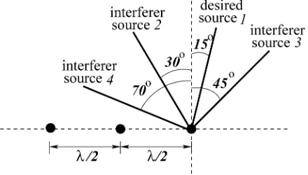
The example consisted of four signal sources and a three-element linear antenna ar-ray. The array element spacing wasλ/2 withλbeing the wavelength. Figure 1 shows the locations of the desired source and three interfering sources graphically. The simulated channel conditions wereAi=αi+j0 for 1i4, withαi>0 so chosen to provide the

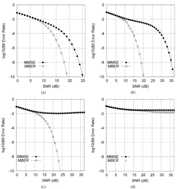
required received signal powers. Figure 2 compares the BER performance of the MBER beamforming assisted receiver with that of the MMSE beamforming assisted receiver un-der four different conditions: (a) the desired user and all the three interfering sources had equal power, (b) the desired user and the interfering users 2 and 3 had equal power but the interfering source 4 had 6 dB more power than the desired user, (c) all the three interfering sources had 2 dB more power than the desired user, and (d) the interfering sources 2 and 4 had 2 dB more power, while the interferer 3 had 6 dB more power, than the desired user. The MMSE solution was calculated using (12) while the MBER solution was determined numerically using the simplified conjugate gradient algorithm presented in Section 3. For this example, the superior performance of the MBER beamforming technique over the MMSE scheme is evident. It can be seen from Figs. 2a–2c that, as the interference signals get stronger, the MMSE beamformer’s performance deteriorates quickly and exhibits an irreducible BER floor. In contrast, the MBER solution shows some degree of robustness to the near-far effect. The first attempt to explain this phenomenon was made by examining the beam pattern used in traditional beamforming.

(a) (b)

(c) (d)

Fig. 2. Comparison of the bit error rates of the MMSE and MBER beamformers for the time-invariant system: (a) SIRi=0 dB fori=2,3,4; (b) SIR2=SIR3=0 dB and SIR4= −6 dB; (c) SIRi= −2 dB fori=2,3,4;

and (d) SIR2=SIR4= −2 dB and SIR3= −6 dB.

The discrete Fourier transform of the beamformer weights, also referred to as the beam pattern, is given by

F (θ )= L

l=1

wlexp

−j ωl(θ )

, (53)

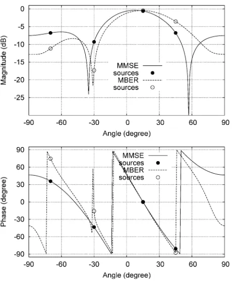
beamform-Fig. 3. Comparison of the MMSE and MBER beam patterns given SNR=15 dB and SIRi=0 dB fori=2,3,4

for the time-invariant system. The weight vector of the MBER solution is scaled to have the same length as the MMSE solution.

ers, respectively, given SNR=15 dB, SIRi =0 dB for i=2,3,4, which illustrates a

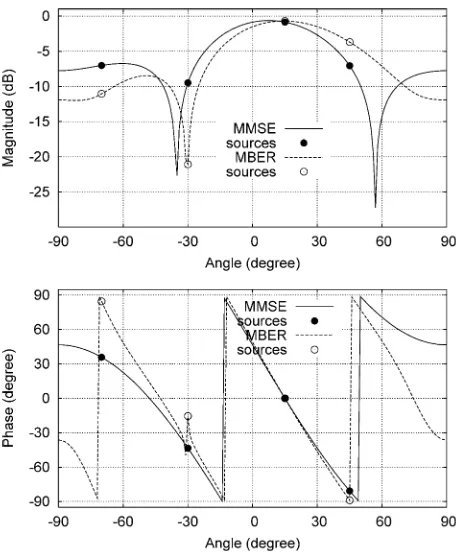
condition represented in Fig. 2a. Figure 4 depicts the corresponding beam patterns given SNR=20 dB, and SIRi= −2 dB fori=2,3,4, which represents a case of the conditions

shown in Fig. 2c. The two beam patterns shown in Fig. 3 do not have big differences and thus it is difficult to explain from the beam pattern why the MBER solution has a much better BER performance than the MMSE scheme, as can be seen from Fig. 2a. Moreover, the beam patterns of Figs. 3 and 4 are similar, which could not explain why the MMSE scheme should have a high BER floor, as shown in Fig. 2c.

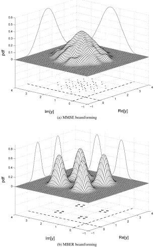
The pdf of the beamformer’s output fully characterizes the true performance of the beamformer. Figures 5 and 6 depict the full conditional pdfp(y|+1+j ), the two marginal conditional pdfsp(yR| +1+j )andp(yI| +1+j )together with the subsetY+,+for the

MMSE and MBER beamformers under the same conditions as given in Figs. 3 and 4, respectively. In these two figures, the beamformer’s weight vector has been normalized to a unit length. It can be seen from Fig. 5 that the minimum distance fromY+,+to the

Fig. 4. Comparison of the MMSE and MBER beam patterns given SNR=20 dB and SIRi= −2 dB fori=2,3,4

for the time-invariant system. The weight vector of the MBER solution is scaled to have the same length as the MMSE solution.

lost linear separability, as can be clearly seen in Fig. 6a, where the two circles mark the points ofY₊,+that have just crossed over to the wrong sides of the decision boundaries.

This explains the irreducible high BER exhibited in Fig. 2c for the MMSE beamformer. In contrast, a desired linear separability is maintained for the MBER beamformer even under such an adverse condition. At the extremely adverse condition given in Fig. 2d, the underlying system becomes linearly inseparable, and any linear beamformer will exhibit a high BER floor. In such a situation, nonlinear beamforming may be employed to achieve an adequate performance at a cost of increased complexity [40].

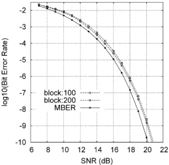
Let us now study the performance of the block-data based gradient adaptive MBER al-gorithm employing the conjugate gradient updating mechanism presented in Section 4.1. The effect of the block sizeKon the performance of this block-data based adaptive MBER algorithm is investigated in Fig. 7, given the condition that the desired user and the inter-fering sources 2 and 3 had an equal power, while the interinter-fering source 4 had a 6 dB higher power than the desired user. Note that for this example, the signal setX contains 256 states, calculated using the formulaNb=4MwithM=4. It is seen that with a short block

(a) MMSE beamforming

(b) MBER beamforming

Fig. 5. Conditional probability density functionsp(y|+1+j )(surfaces), marginal conditional probability density functionsp(yR| +1+j )andp(yI| +1+j )(curves), and signal subsetsY+,+(dots) for the time-invariant

system. SNR=15 dB and SIRi=0 dB fori=2,3,4. The beamformer’s weight vector is normalized to unit

(a) MMSE beamforming

(b) MBER beamforming

Fig. 6. Conditional probability density functionsp(y|+1+j )(surfaces), marginal conditional probability density functionsp(yR| +1+j )andp(yI| +1+j )(curves), and signal subsetsY+,+(dots) for the time-invariant

system. SNR=20 dB and SIRi= −2 dB fori=2,3,4. The beamformer’s weight vector is normalized to unit

Fig. 7. Effect of block size on the performance of the block-data based gradient adaptive MBER algorithm of Section 4.1 for the time-invariant system. SIR2=SIR3=0 dB and SIR4= −6 dB.

Fig. 8. Convergence rate of the block-data based gradient adaptive MBER algorithm of Section 4.1 for the time-invariant system with a block size ofK=400, SNR=17 dB, SIR2=SIR3=0 dB, and SIR4= −6 dB, and given (a): initial w=wMMSE,µ=0.3 andρn2=3σn2≈0.06; and (b): initial w= [0.0+j0.1 0.1+j0.0 0.1+ j0.0]T,µ=0.7, andρn2=3σn2≈0.06.

weight conditions, Fig. 8 illustrates the convergence rates of the block-data based gradient adaptive MBER algorithm. From Fig. 8, it can be seen that this block-data based adaptive algorithm converges rapidly. The step sizeµ and radius parameterρn used were chosen

empirically to ensure a fast convergence speed. The influence of the scaling parameterρ2

n

on the performance of the block-data based adaptive MBER algorithm was investigated in Fig. 9 under the same condition given in Fig. 8b. It can be seen that the performance of the algorithm is not overly sensitive to a large range ofρ_n2values.

Fig. 9. Influence of the scaling parameterρ_n2on the performance of the block-data based gradient adaptive MBER algorithm of Section 4.1 for the time-invariant system with a block size ofK=400, SNR=17 dB, SIR2=SIR3=0 dB, and SIR4= −6 dB, and given w= [0.0+j0.1 0.1+j0.0 0.1+j0.0]T.

It can be seen that this stochastic gradient adaptive MBER algorithm converges reasonably fast. In Fig. 9a, the initial BER was lower than 10−2, which was sufficient low for the DD adaptation. For the condition specified in Fig. 9b, however, 140 samples of training were used first to lower the BER before it switched to the DD adaptation. The adaptive gainµand kernel widthρnwere determined empirically to ensure a good performance in

terms of convergence rate and steady-state BER misadjustment. As expected, initial weight condition affects convergence speed since the BER is a complicated nonlinear function of the weight vector. As a comparison, the learning curves of the LMS algorithm were also shown in Fig. 10. As expected, the BER of the LMS beamforming assisted receiver cannot be lower than that of the MMSE solution.

5.2. Slow-fading system

The locations of the four users were identical to those shown in Fig. 1 but the an-tenna array consisted of fourλ/2-spacing elements. The magnitudes of the 4 channelsAi,

1i4, were independent Rayleigh processes and the associated root mean powers of

Ai were

√

0.5+j√0.5, for 1i4. Continuously fluctuating fading was used at a nor-malized Doppler frequency of 10−6, providing a different fading magnitude and phase for each transmitted symbol. The transmission frame structure consisted of 40 training sym-bols followed by 400 data symsym-bols. The performance of the LBER and LMS beamforming assisted receivers are compared in Fig. 11, where the superior performance of the LBER algorithm over the LMS one is evident. Note that this was not an over loaded system, since the number of the users was four and the number of the receiver antennas was also four.

6. Conclusions

(a) w(0)=wMMSE,µ=0.03, andρn2=3σn2≈0.06

(b) w(0)= [0.0+j0.1 0.1+j0.0 0.1+j0.0]T,µ=0.03, andρn2=3σn2≈0.06

Fig. 10. Learning curves of the stochastic gradient adaptive MBER algorithm of Section 4.2 averaged over 100 runs for the time-invariant system, given SNR=17 dB, SIR2=SIR3=0 dB, and SIR4= −6 dB, where DD: decision-directed adaptation withbˆ1(k)substitutingb1(k).

Fig. 11. Comparison of the bit error rates of the LMS and LBER beamforming assisted receivers for the slow-fading system.

work is required to investigate the general case of wideband channels and to study broad-band beamforming (space-time processing) assisted receiver. Finally, we would also like to point out that the MBER beamforming solution derived for synchronous systems can be extended to asynchronous systems by considering a detection window of three symbols, where the two symbols of the asynchronous interferer overlap with the desired symbol of the reference user. Naturally, this increases the detection complexity. Note that this tech-nique of using a window of three symbols, namely the previous, current and next symbol is a method widely adopted in asynchronous CDMA multiuser detection [41].

References

[1] J.H. Winters, J. Salz, R.D. Gitlin, The impact of antenna diversity on the capacity of wireless communication systems, IEEE Trans. Commun. 42 (2) (1994) 1740–1751.

[2] M.C. Wells, Increasing the capacity of GSM cellular radio using adaptive antennas, IEE Proc. Com-mun. 143 (5) (1996) 304–310.

[3] J. Litva, T.K.Y. Lo, Digital Beamforming in Wireless Communications, Artech House, London, 1996. [4] L.C. Godara, Applications of antenna arrays to mobile communications, Part I: Performance improvement,

feasibility, and system considerations, Proc. IEEE 85 (7) (1997) 1031–1060.

[5] L.C. Godara, Applications of antenna arrays to mobile communications, Part II: Beam-forming and direction-of-arrival considerations, Proc. IEEE 85 (8) (1997) 1193–1245.

[6] A.J. Paulraj, C.B. Papadias, Space-time processing for wireless communications, IEEE Signal Process. Mag. 14 (6) (1997) 49–83.

[7] J.H. Winters, Smart antennas for wireless systems, IEEE Personal Commun. 5 (1) (1998) 23–27.

[9] P. Petrus, R.B. Ertel, J.H. Reed, Capacity enhancement using adaptive arrays in an AMPS system, IEEE Trans. Vehicular Technol. 47 (3) (1998) 717–727.

[10] G.V. Tsoulos, Smart antennas for mobile communication systems: benefits and challenges, IEE Electron. Commun. J. 11 (2) (1999) 84–94.

[11] J.S. Blogh, L. Hanzo, Third Generation Systems and Intelligent Wireless Networking—Smart Antennas and Adaptive Modulation, Wiley, Chichester, 2002.

[12] R.A. Soni, R.M. Buehrer, R.D. Benning, Intelligent antenna system for cdma2000, IEEE Signal Process. Mag. 19 (4) (2002) 54–67.

[13] I.S. Reed, J.D. Mallett, L.E. Brennan, Rapid convergence rate in adaptive arrays, IEEE Trans. Aerospace Electron. Syst. AES-10 (1974) 853–863.

[14] M.W. Ganz, R.L. Moses, S.L. Wilson, Convergence of the SMI and the diagonally loaded SMI algorithms with weak interference (adaptive array), IEEE Trans. Antennas Propagation 38 (3) (1990) 394–399. [15] B. Widrow, P.E. Mantey, L.J. Griffiths, B.B. Goode, Adaptive antenna systems, Proc. IEEE 55 (1967) 2143–

2159.

[16] L.J. Griffiths, A simple adaptive algorithm for real-time processing in antenna arrays, Proc. IEEE 57 (1969) 1696–1704.

[17] S. Haykin, Adaptive Filter Theory, third ed., Prentice Hall, Upper Saddle River, NJ, 1996.

[18] S. Chen, B. Mulgrew, E.S. Cheng, G. Gibson, Space translation properties and the minimum-BER linear-combiner DFE, IEE Proc. Commun. 145 (5) (1998) 316–322.

[19] I.N. Psaromiligkos, S.N. Batalama, D.A. Pados, On adaptive minimum probability of error linear filter re-ceivers for DS-CDMA channels, IEEE Trans. Commun. 47 (7) (1999) 1092–1102.

[20] C.C. Yeh, J.R. Barry, Adaptive minimum bit-error rate equalization for binary signaling, IEEE Trans. Com-mun. 48 (7) (2000) 1226–1235.

[21] B. Mulgrew, S. Chen, Adaptive minimum-BER decision feedback equalisers for binary signalling, Signal Process. 81 (7) (2001) 1479–1489.

[22] S. Chen, A.K. Samingan, B. Mulgrew, L. Hanzo, Adaptive minimum-BER linear multiuser detection for DS-CDMA signals in multipath channels, IEEE Trans. Signal Process. 49 (6) (2001) 1240–1247. [23] S. Chen, L. Hanzo, N.N. Ahmad, Adaptive minimum bit error rate beamforming assisted receiver for

wire-less communications, in: Proc. ICASSP 2003, vol. IV, Hong Kong, China, April 2003, pp. 640–643. [24] E. Parzen, On estimation of a probability density function and mode, Ann. Math. Statist. 33 (1962) 1066–

1076.

[25] B.W. Silverman, Density Estimation, Chapman & Hall, London, 1996.

[26] A.W. Bowman, A. Azzalini, Applied Smoothing Techniques for Data Analysis, Oxford Univ. Press, Oxford, 1997.

[27] M.S. Bazaraa, H.D. Sherali, C.M. Shetty, Nonlinear Programming: Theory and Algorithms, Wiley, New York, 1993.

[28] R. Steele, L. Hanzo, Mobile Radio Communications, IEEE Press, Piscataway, NJ, 1999.

[29] S.-H. Hwang, L. Hanzo, Reverse-link performance of synchronous DS-CDMA systems in dispersive Rician multipath fading channels, IEE Electron. Lett. 39 (23) (2003) 1682–1684.

[30] K. Abend, B.D. Fritchman, Statistical detection for communication channels with intersymbol interference, Proc. IEEE 58 (5) (1970) 779–785.

[31] S. Chen, B. Mulgrew, P.M. Grant, A clustering technique for digital communications channel equalisation using radial basis function networks, IEEE Trans. Neural Networks 4 (4) (1993) 570–579.

[32] S. Chen, B. Mulgrew, S. McLaughlin, Adaptive Bayesian equaliser with decision feedback, IEEE Trans. Signal Process. 41 (9) (1993) 2918–2927.

[33] S. Chen, S. McLaughlin, B. Mulgrew, P.M. Grant, Adaptive Bayesian decision feedback equaliser for dis-persive mobile radio channels, IEEE Trans. Commun. 43 (1995) 1937–1946.

[34] S. Chen, S. McLaughlin, B. Mulgrew, P.M. Grant, Bayesian decision feedback equaliser for overcoming co-channel interference, IEE Proc. Commun. 143 (4) (1996) 219–225.

[35] S. Chen, A.K. Samingan, L. Hanzo, Support vector machine multiuser receiver for DS-CDMA signals in multipath channels, IEEE Trans. Neural Networks 12 (3) (2001) 604–611.

[36] D.E. Goldberg, Genetic Algorithms in Search, Optimization and Machine Learning, Addison–Wesley, Read-ing, MA, 1989.

[38] L. Ingber, Simulated annealing: practice versus theory, Math. Comput. Modeling 18 (11) (1993) 29–57. [39] S. Chen, B.L. Luk, Adaptive simulated annealing for optimization in signal processing applications, Signal

Process. 79 (1) (1999) 117–128.

[40] S. Chen, L. Hanzo, A. Wolfgang, Kernel-based nonlinear beamforming construction using orthogonal forward selection with Fisher ratio class separability measure, IEEE Signal Process. Lett. 11 (5) (2004) 478–481.