Self-Tuning Resource Aware Specialisation for Prolog
Stephen-John Craig
University of Southampton, United Kingdom University of D ¨usseldorf, Germany
[email protected]
Michael Leuschel
∗University of D ¨usseldorf, Germany
[email protected]
ABSTRACT
The paper develops a self-tuning resource aware partial eval-uation technique for Prolog programs, which derives its own control strategies tuned for the underlying computer archi-tecture and Prolog compiler using a genetic algorithm ap-proach. The algorithm is based on mutating the annotations of offline partial evaluation. Using a set of representative sample queries it decides upon the fitness of annotations, controlling the trade-off between code explosion, speedup gained and specialisation time. The user can specify the importance of each of these factors in determining the qual-ity of the produced code, tailouring the specialisation to the particular problem at hand. We present experimental results for our implemented technique on a series of bench-marks. The results are compared against the aggressive ter-mination based binding-time analysis and optimised using different measures for the quality of code. We also show that our technique avoids some classical pitfalls of partial evaluation.
Keywords
Partial Evaluation, Partial Deduction, Binding-Time Ana-lysis,Logic Programming
1.
INTRODUCTION
Despite over 10 years of research on the specialisation of logic programs, there still exist research challenges related to improving the actual specialisation capabilities (this is also true for specialisation of other programming paradigms). For example, existing specialisers do not use a sufficiently precise model of the compiler for the target system to guide their decisions during specialisation. This means that spe-cialisers can produce specialised code that is actually slower
∗The authors have been partially supported by the Infor-mation Society Technologies programme of the European Commission, Future and Emerging Technologies under the IST-2001-38059 ASAP project.
Permission to make digital or hard copies of all or part of this work for personal or classroom use is granted without fee provided that copies are not made or distributed for profit or commercial advantage and that copies bear this notice and the full citation on the first page. To copy otherwise, to republish, to post on servers or to redistribute to lists, requires prior specific permission and/or a fee.
Copyright 200X ACM X-XXXXX-XX-X/XX/XX ...$5.00.
than the original. Also, most specialisers focus solely on im-proving the execution speed, sacrificing other resources such as code size and memory consumption. This means that the code size and specialisation effort can be out of proportion with the actual improvement in speed.
Developing control techniques that are predictable, with reasonable specialisation complexity and that can provide a good balance between resources, is a challenging but worth-while research objective.
In this paper we present aself-tuning system, which de-rives its own specialisation control using a genetic algorithm approach.
Fitness scores are derived by actually running the spe-cialised code and hence the particular Prolog compiler and architecture are automatically taken into account.
More precisely, we use an offline approach based on the recent fully automatic binding-time analysis (BTA)[5]. The insight on which this paper is based, is that the annotations can form the genes for a genetic algorithm.1
Indeed, an-notations can easily be mutated, or even merged. The key ingredients of success in our approach are:
• The fully automatic BTA provides a starting point for the algorithm. The BTA can be used to check the safety of new annotation configurations. Alternatively, based on the starting point provided by the BTA, a time-out value can be computed which can be used to discard unsuccessful mutations (where specialisation takes too long or does not terminate).
• Overall termination and convergence is guaranteed as mutations only “generalise” (unfold into memo, static into dynamic).
• Through the use of a representative sample of queries, actual figures for the particular compiler and archi-tecture are obtained. This allows for resource aware specialisation.
• The overall tradeoff between execution time, code size (and other factors such as specialisation time) can be influenced by tuning the fitness function, used to dis-card bad mutations.
This paper, shows, empirically and through examples, how it avoids pitfalls which other specialisers such asecce [16] or mixtus [21] fall into. We also show how we can
1
achieve a good tradeoff between various resource consider-ations. It is also demonstrated on a series of benchmark programs the practicality and performance of the approach.
1.1
Other Approaches and Related Work
Such an approach has already proven to be highly suc-cessful in the context of optimising scientific linear algebra software [25]. In [25] part of the installation procedure in-cludes a test and feedback cycle which optimises internal parameters to give the best performance for the processor architecture, memory and cache.A suitablelow-level cost modelwould allow a partial evalu-ation system to make more informed choices about the local control (e.g., is this unfolding step going to be detrimen-tal to performance) and global control (e.g., does this extra polyvariance really pay off).
There has been some promising initial work on cost mod-els for logic and functional programs in [1, 2, 24, 4]. How-ever, such a low-level cost model will depend on both the particular Prolog compiler and on the target architecture and it is hence unlikely that one can find an elegant math-ematical model that is easy to manipulate and precise. It is also not entirely clear how such a cost model could be used in practice to guide specialisation. It is possible that the approach we present in this paper could make use of a low-level cost model to determine the quality of specialised code, but a cost model may prove too inaccurate to give reliable results.
2.
CONTROLLING PARTIAL DEDUCTION
In the remainder of the paper we assume some basic know-ledge of logic programming [17].
2.1
Basics of Partial Deduction
Partial deduction [18] is a program specialisation tech-nique for logic programs: given a logic programP and some partially instantiated queryQ, it derives a new programP′, which is specialised for answering the queryQ and all its possible instantiations. Partial deduction proceeds by de-riving a set of atoms A and by building for each element ofAa possibly incomplete SLDNF-tree using anunfolding rule. For every element ofA, partial deduction produces a specialised predicate definition by extracting a specialised clause from every non-failing branch of the tree built for it. An important issue in partial deduction is the control. Here we distinguish between [19]
– global control: deciding which atoms to be put intoA, and
– local control: deciding which trees to build for the elements ofA.
The issue of control is important as it affects the correctness and termination of the specialisation process, as well as the quality of the specialised program. Considerable effort has been devoted to this crucial issue (see, e.g., the references in [14]), and the issue of correctness is well understood and several powerful techniques (such as homeomorphic embed-ding) can be used to ensure termination. However, the issue of the quality of the specialised program is still relatively open. While it is well understood that unrestricted unfold-ing can be detrimental to the efficiency of the specialised program, and that determinate unfolding can be used to avoid most pitfalls related to this, the overall picture is un-clear. Indeed, using just determinate unfolding will prevent
substantial efficiency gains in certain cases, and still may not prevent program slowdowns and code explosion (with a limited efficiency gain). Below we elaborate on some of the pitfalls of partial deduction in more detail, showing where it can go wrong and produce undesirable results.
2.2
Some Pitfalls of Partial Deduction
One pitfall related to the local control (unfolding) is known as work duplication. The problem is illustrated in the fol-lowing example.
LetP be the program defined in Listing 1.
member ( X ,[ X | T ]).
member ( X ,[ Y | T ]) : - member (X , T ). inboth ( X , L1 , L2 ) : - member (X , L1 ) ,
member (X , L2 ).
Listing 1: The inboth/3 example
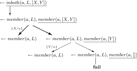
Let A= {inboth(a,L,[X,Y]), member(a,L)}. By per-forming non-leftmost non-determinate unfolding for the call
inboth(a,L,[X,Y]) in Figure 1 (and doing a single unfold-ing step for member(a,L)), we obtain the partial deduction P′ (Listing 2) ofP with respect toA.
member ( a ,[ a | T ]).
member ( a ,[ Y | T ]) : - member (a , T ). inboth ( a ,L ,[ a , Y ]) : - member (a , L ). inboth ( a ,L ,[ X , a ]) : - member (a , L ).
Listing 2: Specialising Listing 1 for
{inboth(a,L,[X,Y]), member(a,L)}
Let us examine the run-time goalG=←inboth(a,[h,g,f, e,d,c,b,a],[X,Y])(which is an instance of an atom inA). Using the Prolog left-to-right computation rule the expen-sive sub-goal←member(a,[h,g,f,e,d,c,b,a])is only eval-uated once in the original program P, while it is executed twice in the specialised programP′.
H H
HHj
fail
←member(a, L),member(a,[]) ←member(a, L)
←member(a, L),member(a,[Y])
HHH
H j
←member(a, L)
←member(a, L),member(a,[X, Y])
?
←inboth(a, L,[X, Y])
{X/a}
[image:2.595.323.559.444.567.2]{Y /a}
Figure 1: Non-leftmost non-determinate unfolding for Listing 2
The classical solution to this problem is to disallow non-leftmost unfolding unless it is deterministic (sp [7, 8, 9], ecce [16]), or allow non-leftmost unfolding but not left-propagate bindings (paddy[20],mixtus[21]). Some partial evaluators, for instance, sage [11, 10] do not prevent such work duplication. This can result in huge slowdowns (see, e.g., [3]).
unfolding can still lead to duplication of work, namely in unification with multiple heads:
Let us return to the program in Listing 1 with the setA=
{inboth(X,[Y],[V,W])}. The query can be fully unfolded producing the partial deduction P′ (Listing 3) of P with respect toA.
inboth (X ,[ X ] ,[X , W ]). inboth (X ,[ X ] ,[V , X ]).
Listing 3: Specialising Listing 1 for
{inboth(X,[Y],[V,W])}
No goal has been duplicated by the leftmost non-determinate unfolding, but the unificationX=Yfor←inboth(X,[Y],[V,W])
has been duplicated in the residual code. This unification can have a substantial cost when the corresponding actual terms are large.
Another trap of partial deduction is the possible loss of indexing. Indeed, Prolog systems spend a lot of their time looking up clauses that match the current goal. When all calling arguments are free, the system has no choice but to go through the clauses one by one. However, if some of the arguments are (at least partially) instantiated then some clauses that do not match can be skipped. This is achieved using argument indexing and takes analogy from indexing in database systems. The standard Prolog indexing techniques rely onfirst argument clause indexing; that is they by de-fault index on the first argument. Indexing can provide an important performance boost when searching over a large set of clauses.
Listing 4 is a a simple program with a collection of facts represented byp/2. By default indexing will be performed on the first argument ofp/2, and as long as the first argu-ment in the call top/2is instantiated we will benefit from the speedups of indexing.
i n d e x _ t e s t( f ( _ ) ,Y , Z ) : - p (Y , Z ). p (a ,1).
p (b ,2). p (c ,3). p (d ,4). p (e ,5). p (f ,6). p (g ,7). p (h ,8). p (i ,9). p (j ,10).
Listing 4: Example using clause indexing
During specialisation unfolding may change the behaviour of the clause indexing. Through unfolding, facts may be subsumed by calling predicates, whose argument orderings differ. When specialising Listing 4 forindex test(A,B,C)it is safe to fully unfold the call top/2, as termination is guar-anteed and it removes a level of redirection. Unfortunately in the newly createdindex test 0/3predicate (Listing 5), the first argument is no longer a useful basis for clause in-dexing and as a result, the specialised code is substantially slower than the original program (taking twice as long to complete the same benchmark).
i n d e x _ t e s t _ _ 0( f ( _ ) , a , 1). i n d e x _ t e s t _ _ 0( f ( _ ) , b , 2). i n d e x _ t e s t _ _ 0( f ( _ ) , c , 3). i n d e x _ t e s t _ _ 0( f ( _ ) , d , 4). i n d e x _ t e s t _ _ 0( f ( _ ) , e , 5). i n d e x _ t e s t _ _ 0( f ( _ ) , f , 6). i n d e x _ t e s t _ _ 0( f ( _ ) , g , 7). i n d e x _ t e s t _ _ 0( f ( _ ) , h , 8).
i n d e x _ t e s t _ _ 0( f ( _ ) , i , 9). i n d e x _ t e s t _ _ 0( f ( _ ) , j , 10).
Listing 5: Specialising Listing 4 for
index test(A,B,C). The useful clause indexing has been lost
In Ciao Prolog (and some others), the indexer allows pro-grammers to select the argument(s) to index on. This would be an alternative to not unfolding the call, but would still require that the specialiser changes the indexing informa-tion. The classical solution is to avoid any reordering of arguments, but this is not enough to prevent this problem. Using pure determinate unfolding (no non-determinate un-folding except at the root of an SLD-tree) together with no argument reordering avoids most of the problems. However, most determinate unfolding rules are not pure and allow one non-determinate step, this is often important for precision (see benchmarks in [16]).2
Another related problem is the loss of indexing due to argument filtering. For example, take the following program:
p(f(a,b)). p(f(b,c)). p(f(d,e)). p(f(e,a)).
Specialising for p(f(X,Y)) produces the following spe-cialised code:
p__1(a,b). p__1(b,c). p__1(d,e). p__1(e,a).
Filtering has removed thef/2 structure and replaced it with two arguments representing the substructure. Now, potentially the specialised program will run slower for a runtime query such as p(f(X,a)), provided the underlying Prolog system provides “deep” indexing (e.g., Ciao Prolog does allow this with the indexer package). This is because only the first argument is indexed, and the lookup is on the second argument in the specialised program. However, most Prolog systems only index on the top-level functor (e.g., SIC-Stus) and hence there is actually no slow-down. In fact the program can run faster as the functorf/2 no longer needs to be deconstructed.
The behaviour of the indexing in different Prologs is a case where depending on the Prolog the specialiser could behave differently to produce better quality code. Prolog systems also impose a maximum number of arguments. Some Pro-log systems do not, but after a certain limit (e.g., 32) all further arguments are simply put into a list. As argument filtering can increase the number of arguments, this must be taken into account by the specialiser. Other differences may exist between Prologs and platforms, for example features such as tabling may influence the performance of specialised programs.
In this section we have only scratched the surface of vari-ous ways in which existing partial deduction techniques can go wrong (more pitfalls can be found in [23], most of which are still valid today). Also, even when partial deduction
2
does achieve some speed improvement, this may ensue an unacceptable explosion in the code size. It is clear that de-riving a good specialised program is a non-trivial pursuit, covered with many pitfalls and difficult to put into a simple mathematical model.
The motivation of this paper is to provide a method for deriving specialisation control based on the underlying ar-chitecture guided by trial and error, providing the user with the ability to balance execution time against code explosion, or other program properties. The algorithm uses empirical measurements to tackle issues that could prove difficult to handle using a purely mathematical model. We concentrate on offline partial deduction as it provides a clear separation between specialisation and control.
3.
OFFLINE PARTIAL DEDUCTION
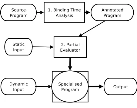
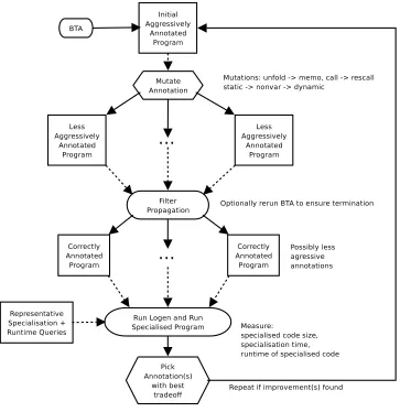
The main idea of offline partial deduction is to separate the specialisation process into two phases:
– First abinding-time analysis(BTA) is performed which, given a program and an approximation of the input available for specialisation, approximates all values within the program and generates anannotated program. – A (simplified)specialisation phase, which is guided by
the annotations of the BTA.
This approach is illustrated in Figure 2 and is calledoffline
because most control decisions are taken beforehand.
Figure 2: Offline Partial Evaluation
In the remainder of the paper we will use thelogen spe-cialisation system [15]. Inlogen every program point in every clause is annotated with a clause annotation, telling the specialiser what to do when reaching this program point. Furthermore, every argument of every predicate is anno-tated with a binding type, which tells the specialiser to what extent this argument will be known at specialisation time.
Clause Annotations
Clause annotations indicate how each call in the program should be treated during specialisation. Essentially, these annotations determine whether a call in the body of a clause is performed at specialisation time or at run time. Clause
annotations influence the local control [19]. For the lo-gen system [15] the main annotations are as follows:
• unfold: The call is unfolded under the control of the partial evaluator. The call is replaced with the pred-icate body, performing all the needed substitutions. (Note: the predicate body is itself annotated and will be re-examined by the partial evaluator.)
• memo: The call is not unfolded, but instead the call is generalised using the filter declaration and specialised independently.
• call: The call is fully executed without further inter-vention by the partial evaluator.
• rescall: The call is left unmodified in the residual code.
Binding Types
Each argument of a predicate in an annotated program is given abinding typeby means offilter declarations. A bind-ing type indicates somethbind-ing about the structure of an argu-ment at specialisation time. This information is used when the predicate is “memoed.” The basic binding types are usually known as static and dynamic which are defined as follows:
• static: The argument is definitely known at speciali-sation time;
• dynamic: The argument is possibly unknown at spe-cialisation time.
More precise binding types can be defined by means of reg-ular type declarations, and combined with basic binding types. For example, one can define types such as list skele-tons.
The filter declarations influence the global control, since
dynamicparts of arguments are generalised away (that is, re-placed by fresh variables) and the known,staticparts are left unchanged. They also influence whether arguments are “fil-tered out” in the specialised program. Indeed, static parts are already known at specialisation time and hence do not have to be passed around at runtime.
The paper [5] introduced an automatic binding-time ana-lysis for logen. The analysis used state-of-the-art termi-nation analysis techniques, combined with a type-based ab-stract interpretation for propagating the binding types com-bined. Safety of built-ins was guaranteed using a database of allowed calling patterns (with respect to the propagated binding types). The analysis was designed to be as aggres-sive as possible and is guided only by termination, it contains no heuristics for quality of code. The algorithm described in this paper is designed to complement the binding-time analysis of [5], providing control over the quality of the pro-duced specialised programs.
[image:4.595.60.286.356.534.2]The recursive call in the secondmatch1/4 clause has been marked memo and cannot be safely unfolded.
match(Pat,T) :−
match1(Pat,T,Pat,T) | {z }
unfold
.
match1([], Ts, P, T).
match1([A|Ps],[B|Ts],P,[X|T]) :−
A\==B,
| {z }
rescall
match1(P,T,P,T).
| {z }
memo
match1([A|Ps],[A|Ts],P,T) :−
match1(Ps,Ts,P,T).
| {z }
unfold
:−filter match(static,dynamic).
[image:5.595.54.236.90.210.2]:−filter match1(static,dynamic,static,dynamic).
Figure 3: Annotated match program
Using the above annotation and the specialisation query
match([a,c], A), logen will produce the following spe-cialised program:
match ([ a , c ] , A ) : - match__0 ( A ). match__0 ([ A | B ]) :
-a \== A , m a t c h 1 _ _ 1(B , B ). match__0 ([ a , A | B ]) :
-c \== A , m a t c h 1 _ _ 1([ A | B ] , [ A | B ]). match__0 ([ a , c | _ ]).
m a t c h 1 _ _ 1([ A | _ ] , [ _ | B ]) : -a \== A , m -a t c h 1 _ _ 1(B , B ). m a t c h 1 _ _ 1([ a , A | _ ] , [ _ | B ]) :
-c \== A , m a t -c h 1 _ _ 1(B , B ). m a t c h 1 _ _ 1([ a , c | _ ] , _ ).
Listing 6: Specialising match/2 using the annota-tions in Figure 3
4.
MUTATIONS
Offline specialisation takes an annotated program as in-put. In this section we examine how annotations can be mu-tated and thus form the basis of a genetic algorithm aimed at improving annotations.
A single set of annotations for a program is represented by an annotation configuration (Definition 1).
Definition 1 (annotation configuration). (α, β)is an annotation configuration for some programP whereα∈
Σ∗c,Σ
c={u, m, c, r}, β∈Σ∗f,Σf ={s, d}
The length of α is the number of body literals in P and the length ofβ is the sum of the arity of the predicates in
P. A configuration represents a set of annotations for the programP. Withu, m, c, r, s, andd representing unfold, memo, call, rescall, static and dynamic respectively.
For example, the annotations from the match program (Figure 3) are represented by the annotation configuration ((u, r, m, u,),(s, d, s, d, s, d)).
The binding-time analysis concentrates on termination and provides a set of aggressive annotations, doing as much work as possible at specialisation time. However, this does not always produce the best specialised programs. As al-ready discussed, there are some circumstances where it is
better not to perform an operation at specialisation time or to discard some static information.
The algorithm presented searches for “better” annotation configurations which, while less aggressive than the configu-ration provided by the binding-time analysis, may produce better specialised code. The algorithm explores the possible
mutations (Definition 2) of the current annotation configu-ration. A mutation of a configuration is defined as a new annotation configuration but with one of the annotations modified. The mutations produce new, less aggressive anno-tations. For example, a call marked as unfold can be turned into memo, or an argument that was previously static is treated as dynamic. This changes the behaviour of the spe-cialiser.
Definition 2 (mutation). LetCbe a annotation con-figuration forP,fcandff are mapping functions defined as
fc ={u7→m, c 7→r}, ff ={s 7→d}. IfC is of the form
(αXα′, β) andX∈dom(fc) then the annotation
configura-tion(αfc(X)α′, β) is a mutation ofC. IfC is of the form (α, βXβ′)andX∈dom(ff)then the annotation
configura-tion(α, βf(X)β′)is a mutation ofC.
Definition 3 (set of mutations). mutations(C)is de-fined as the set of all possible mutations ofC.
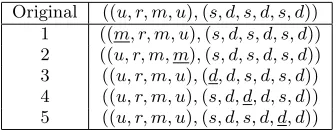
Table 1 shows the initial set of mutations for the match program in Figure 3. The initial configuration of match has five possible mutations, the mutated element has been underlined in each mutation.
[image:5.595.353.521.373.438.2]Original ((u, r, m, u),(s, d, s, d, s, d)) 1 ((m, r, m, u),(s, d, s, d, s, d)) 2 ((u, r, m, m),(s, d, s, d, s, d)) 3 ((u, r, m, u),(d, d, s, d, s, d)) 4 ((u, r, m, u),(s, d, d, d, s, d)) 5 ((u, r, m, u),(s, d, s, d, d, d))
Table 1: Initial set of mutations for match
It is possible that a mutated annotation configuration may be unsafe. Generalising more arguments, or memoising rather than unfolding calls, may have repercussions through-out the rest of the program. The annotation configuration may be unsafe for a number of reasons:
- The filter information may be incorrect. Marking an argument as dynamic or memoing a call rather than unfolding may change the propagation of static data throughout the program.
- A built-in that was previously safe to call, may now not be sufficiently instantiated at specialisation time.
- The specialisation process may fail to terminate. In-formation that previously guaranteed termination may have been generalised away.
The entire binding-time analysis algorithm is complex; however, it is sufficient to run only the filter propagation and built-in safety checking. Non-termination of the spe-cialisation process can then be monitored using timeouts. A sensible value for the timeout can be estimated using the specialisation and runtime of the original annotated program as a base.
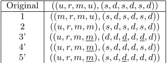
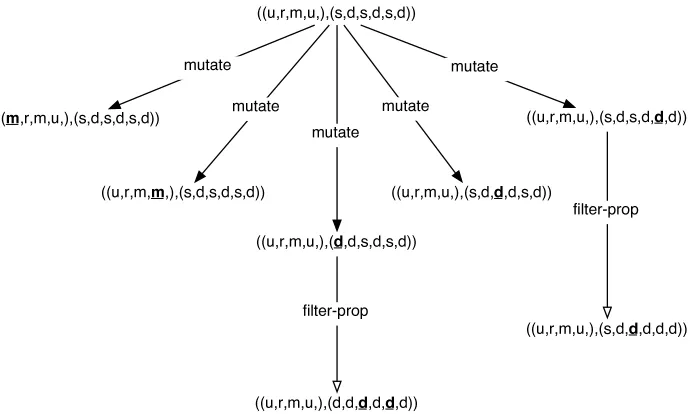
Using the filter propagation and built-in checking on the annotations in Table 1 produces the new safe annotations in Table 2.
[image:6.595.89.258.168.235.2]Original ((u, r, m, u),(s, d, s, d, s, d)) 1 ((m, r, m, u),(s, d, s, d, s, d)) 2 ((u, r, m, m),(s, d, s, d, s, d)) 3’ ((u, r, m, u),(d, d, d, d, d, d)) 4 ((u, r, m, u),(s, d, d, d, s, d)) 5’ ((u, r, m, u),(s, d, d, d, d, d))
Table 2: Mutation after filter propagation
Two of the mutations have been detected as unsafe and have been modified accordingly. Figure 4 shows the tree of these mutations. Running the filter propagation has fur-ther mutated the annotation configuration producing new configurations with multiple mutated elements.
It is also possible to run the full binding-time analysis algorithm to find the safe set of mutations (Table 3). The termination analysis has detected that, in additional to the filters, one of the annotations must be changed from unfold to memo.
Original ((u, r, m, u),(s, d, s, d, s, d)) 1 ((m, r, m, u),(s, d, s, d, s, d)) 2 ((u, r, m, m),(s, d, s, d, s, d)) 3’ ((u, r, m, m),(d, d, d, d, d, d)) 4’ ((u, r, m, m),(s, d, d, d, s, d)) 5’ ((u, r, m, m),(s, d, d, d, d, d))
Table 3: Mutation after full automatic binding-time analysis
5.
DECIDING FITNESS
To explore the search space effectively, it is essential to be able to assess the quality of a particular annotation configu-ration. Empirical testing is used to determine the quality of the specialised code. However, each annotation configura-tion can be used to specialise the same program for different sets of static data. It is impractical to test for all possible sets of of static data, so instead a representative set of sam-ple queries is used. These queries are provided by the user. It is important that the sample queries accurately reflect the type of queries of interest as the program will be optimised with these queries in mind.
The quality of the annotation configuration is calculated using characteristics from the specialisation process:
execution time – The actual execution time of the sample queries. The sample queries are benchmarked over a number of executions to obtain a final execution time.
This allows the algorithm to optimise for the fastest program.
compiled code size – The size of the produced specialised code. The size is taken after compilation into byte code. Specialisation can result in large code explosion, sometimes for a very small gain.
specialisation time – The time taken to specialise the pro-gram for the sample queries. In situations where the program is to be re-specialised frequently it may be desirable to take into account the actual specialisation time during optimisation.
It would be possible to measure additional characteris-tics that may be of interest to the user. For example, the memory usage during execution.
The different characteristics contain different units and cannot easily be combined. To allow comparison between the different characteristics, they are first normalised. Nor-malising the values against a common base case produces a new value, where 1.0 signifies it is the same as the base case, a value of 2.0 indicates it is twice as good as the base case and a value of 0.5 indicates it is twice as bad as the base case.
A fully dynamic annotation configuration (Definition 4) with all calls marked as rescall or memo is used as a base case. The fully dynamic annotation configuration produces specialised code which has the same behaviour as the orig-inal program, as all static data is discarded during special-isation and no calls are made at specialspecial-isation time. Each characteristic is normalised by dividing the value with the same characteristic from the dynamic annotation configura-tion.
Definition 4 (dynamic annotation configuration).
The annotation configuration (α, β) is fully dynamic if α∈
Σ∗
c′,Σc′ ={m, r}, β∈Σ∗f′,Σf′ ={d}.
Where the length ofαis the number of body literals inP
and the length ofβ is the sum of the arity of the predicates inP.
While it would be possible to optimise the program for a single characteristic, much more interesting optimisations can be made by combining the different characteristics into a single score.3
A fitness function (Definition 5) is used to determine the score given the characteristics.
Definition 5 (fitness function). The fitness func-tion is used to determine the qualityof an annotation con-figuration based on its measured characteristics. The func-tion takes as input the normalised values for specialisafunc-tion time (spectime), execution (speedup) and code size reduc-tion (reduction).
The choice of fitness function is important in determin-ing the quality of code for the particular requirements. The fitness function is used to balance the tradeoff between the different characteristics. A simple scoring function to find fastest specialised program would only take into account the execution time. However, sometimes the most aggressive an-notations can cause dramatic code explosion with little ac-tual gain in execution time. Using a scoring function based 3
[image:6.595.89.258.394.458.2]((m ,r,m ,u ,),(s ,d ,s ,d ,s ,d ))
((u ,r,m ,m ,),(s ,d ,s ,d ,s ,d ))
((u ,r,m ,u ,),(d ,d ,s ,d ,s ,d ))
((u ,r,m ,u ,),(s ,d ,s ,d ,d ,d ))
((u ,r,m ,u ,),(s ,d ,d ,d ,s ,d )) m utate
m utate
m utate
m u tate
m u tate
((u ,r,m ,u ,),(d ,d ,d ,d ,d ,d ))
((u ,r,m ,u ,),(s ,d ,d ,d ,d ,d )) filte rp ro p
[image:7.595.134.479.54.261.2]filte rp ro p
Figure 4: Safe annotation configurations after filter propagation
on both the execution time and compiled code size ensures a balance is maintained between the two characteristics.
For example, say the original program executes in 200ms and is 4,000 bytes. Annotation configurationAexecutes in 100ms and is 30,000 bytes while annotation configuration B executes in 120ms but is only 5,000 bytes. It may be desirable to chooseB, which while slightly slower is much smaller thanA.
Currently the default fitness function is defined as score
=speedupα×reductionβ×spectimeγ where theα, βandγ values reflect the importance of the characteristics.
6.
ALGORITHM
Using the concepts defined in the previous sections the complete algorithm is now presented. The algorithm is given an initial starting annotation configuration and returns the best annotation configurations found according to the set fitness function.
To explore the search space the algorithm uses a beam search. The beam search explores the neighbours at each node (in this case the single mutations), and only descends into theW best nodes for each level, whereW is described as the width of the beam. The search terminates when the W best nodes remain unchanged through an iteration.
Figure 5 demonstrates the beam search for W = 2. The values in the nodes represent the scores, a higher score repre-senting a better selection. At each level the search proceeds by selecting the best two solutions.
Figure 6 outlines the algorithm. Starting with an initial annotated program, the algorithm proceeds to find muta-tions of the initial configuration. Each mutation is checked for safety by running the filter propagation and then the safe configurations are benchmarked. At each iteration the best annotations are chosen and the algorithm continues. When no further improvements are found, the algorithm terminates. The depth of the search tree is bounded by the number of annotations, as at each generation at least one annotation must be made less aggressive. The filter
propa-Figure 5: Beam search forW = 2
gation allows multiple annotations to be modified in a single step, effectively skipping levels in the search tree.
Algorithm 1 describes the self-tuning algorithm in psuedo code. It uses Definition 6 to measure the characteristics of an annotation configuration.
Definition 6 (test conf). Given a programP, an an-notation configuration C, a specialisation goal Gsp and a runtime queryGrt, test conf(P, C, Gsp, Grt)returns the tu-ple(ST, RT, SS). WhereST is the time taken to specialise
P for the goal Gsp, producing the specialised program P′. RT is the execution time ofP′ for the goal Grt andSS is
the compiled code size ofP′
For example, running the algorithm on theindex test/3
example (Listing 4) produces the annotations in Figure 7. The annotations have be tuned for time and speed. The algorithm has discovered that the call should not be unfolded (as it is detrimental to performace) and has marked it as memo. The tuned annotations produced specialised code that is twice as fast as the aggressive annotations.
[image:7.595.344.527.313.433.2]Figure 6: Self-tuning overview
index test(f( ),Y,Z) :−p(Y,Z) | {z }
memo .
. . .
Figure 7: Final annotations for index test/3, opti-mised for time and size
has decided that while the first call can be safely unfolded, better code can be produced by memoing the call instead. The produced code is nearly two times smaller than the aggressive annotations and runs faster (full details can be found in Table 4).
7.
EXPERIMENTS
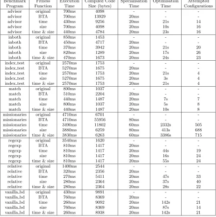
Table 4 presents the results of running4
the self-tuning algorithm on a series of benchmarks taken from the DPPD library [13]:
advisor – A simple expert system.
inboth – The inboth example form Section 2.2.
4
Benchmarks were performed on a 2.5Ghz Pentium with 512MB running SICStus Prolog 3.11.1
match(Pat,T) :−
match1(Pat,T,Pat,T) | {z }
memo
.
match1([], Ts, P, T).
match1([A|Ps],[B|Ts],P,[X|T]) :−
A\==B,
| {z }
rescall
match1(P,T,P,T).
| {z }
memo
match1([A|Ps],[A|Ts],P,T) :−
match1(Ps,Ts,P,T).
| {z }
unfold
:−filter match(static,dynamic).
:−filter match1(static,dynamic,static,dynamic).
Figure 8: Final annotations for match/2, optimised for time and size
index test – The indexing example from Section 2.2.
match – A simple na¨ıve pattern matcher.
Algorithm 1Self-tuning algorithm
Input:ProgramP
Input:Initial annotation configurationCinit
Input:Specialisation goalGsp
Input:Runtime goalGrt
Input:Beam widthW
1: Cdyn= fully dynamic annotation configuration forP 2: (STdyn, RTdyn, SSdyn) = TestConf(P,Cdyn,Gsp,Grt) 3: Cache={Cdyn7→fitness func(1,1,1)}
4: CS ={Cinit}
5: repeat
6: CSsafe =CS 7: for allC∈CSdo
8: msafe = safe set ofmutations(C) 9: CSsafe=CSsafe∪msafe
10: end for
11: for allC∈CSsaf edo
12: if C /∈dom(Cache)then
13: (ST, RT, SS) = TestConf(P,C,Gsp,Grt) 14: ST′ =ST /STdyn
15: RT′ =RT /RTdyn 16: SS′ =SS/SSdyn
17: Score=fitness func(ST′, RT′, SS′) 18: Cache=Cache∪ {C7→Score}
19: end if
20: end for
21: Previous =CS
22: CS = Choose bestW configurations based on scores fromCache
23: untilCS=Previous
regexp – A program testing whether a string matches a regular expression (using difference lists).
relative – A simple expert system.
vanilla bd – A vanilla meta-interpreter, with a “contrived” object program invented by Bart Demoen.
Each test program has five enteries in the table: the orig-inal program, the program after specialising it using the an-notations derived by the BTA of [5], and the results from the self-tuning algorithm with three different fitness functions:
time – The normalised time to execute the specialised pro-gram. score=speedup.
size – The normalised size of the byte compiled specialised program. score=reduction.
time& size – An equally weighting of the normalised ex-ecution time and program size. score = speedup×
reduction.
The execution time, compiled code size and specialisation time are the non-normalised characteristics from Section 5. The optimisation time is the total time taken to find the annotation configuration, the starting configurations were provided by the BTA. The number of attempted configu-rations is the actual number of different annotations that were tested during the search. Note, the three enteries for the different fitness functions were timed independently of each other, in practice the cache could be reused for the different searches.
The results show that the highly aggressive configurations provided by the termination driven binding-time analysis do not neccessarily produce the best code, either in terms of code size or execution time. In both themissionariesand ad-visorexamples the BTA configuration suffers from a code ex-plosion for no actual gain. Themissionariesexample suffers an eight-fold increase in size, while the advisor example is three times larger; with neither program running any faster. The aggressive unfolding in theindex testexample also suf-fers a performance penalty, the loss of the clause indexing causes the BTA configuration to run two times slower than the original. Another interesting example isvanilla demoen. The purpose of the example was to show that under some circumstances meta-interpretation has the advantage of cre-ating terms late and that removing the meta-interpretation can actually slow down the program. Our algorithm here has avoided the pitfall and has actually found a speciali-sation that improves upon the original but does not suffer from the problem of creating terms too early.
Solely using execution time as a measure for the qual-ity of code is not always ideal either. The advisor, inboth,
missionariesandrelativeexamples all suffer from an explo-sion in code size when optimised only for execution time. Balancing execution time against code size produces some interesting results. For example, themissionariesprogram’s fastest solution is 35% faster than the original with an 75% increase in code size; balancing code size with execution time finds a solution which is 23% faster than the original and is also actually 7% smaller. In the three other examples, the comprimise solution finds configurations which perform marginally slower than the fastest, but without the code explosion.
8.
SUMMARY AND FUTURE WORK
This paper has presented a self-tuning, resource-aware of-fline specialisation technique. The main insight was that the annotations of offline partial evaluation can be used as the basis of a genetic algorithm. Indeed, the fitness of an-notations can be evaluated by trial and error using a set of representative sample queries on some target Prolog system and hardware, taking properties such as execution time and code size into account. This makes our approach both re-source aware and able to fine-tune itself to new hardware or Prolog systems. Furthermore, annotations can be mutated by toggling individual clause or predicate annotations. To reduce the search space we make use of a recent fully au-tomatic binding-time analysis [5] in order to adapt unsafe mutations (of which there are many) into safe ones. The binding-time analysis also provides a valid starting point for our algorithm.
The empirical evaluation or our technique has been very encouraging. We have shown that our self-tuning algorithms avoids pitfalls of ordinary partial evaluation, while being able to find better specialised code in terms of speedup, code size or both. For example, the results show that the binding-time analysis of [5] can lead to large code explosion for little gain in efficiency, while our algorithm finds a much better tradeoff.
con-Benchmark Fitness Execution Compiled Code Specialisation Optimisation Attempted Program Function Time Size (bytes) Time Time Configurations
advisor original 700ms 4098 - -
-advisor BTA 700ms 13929 20ms -
-advisor time 430ms 9256 20ms 21s 14
advisor size 700ms 4098 20ms 10s 16
advisor time & size 440ms 4784 20ms 23s 16
inboth original 850ms 1453 - -
-inboth BTA 450ms 4717 20ms -
-inboth time 370ms 3942 20ms 21s 20
inboth size 820ms 1289 20ms 17s 26
inboth time & size 470ms 1673 20ms 24s 23
index test original 2570ms 1753 - -
-index test BTA 5270ms 1675 20ms -
-index test time 2570ms 1753 20ms 21s 4
index test size 5270ms 1675 20ms 3s 4
index test time & size 2570ms 1753 20ms 21s 4
match original 800ms 1037 - -
-match BTA 510ms 2204 20ms -
-match time 440ms 1487 20ms 7s 7
match size 800ms 1037 20ms 5s 8
match time & size 440ms 1487 20ms 10s 8
missionaries original 4710ms 6701 - -
-missionaries BTA 4710ms 55956 80ms -
-missionaries time 3490ms 11802 60ms 2332s 505
missionaries size 3880ms 6259 80ms 413s 688
missionaries time & size 3830ms 6263 60ms 3386s 715
regexp original 3540ms 1620 - -
-regexp BTA 810ms 1417 20ms -
-regexp time 810ms 1417 20ms 44s 19
regexp size 810ms 1417 20ms 16s 24
regexp time & size 810ms 1417 20ms 55s 24
relative original 1400ms 2544 - -
-relative BTA 320ms 2356 20ms -
-relative time 270ms 5411 20ms 47s 33
relative size 280ms 2364 20ms 37s 40
relative time & size 280ms 2364 20ms 28s 22
vanilla bd original 430ms 9891 - -
-vanilla bd BTA 760ms 8369 20ms -
-vanilla bd time 260ms 9092 20ms 142s 21
vanilla bd size 760ms 8369 20ms 87s 14
[image:10.595.85.525.57.500.2]vanilla bd time & size 260ms 8938 20ms 142s 21
Table 4: Experimental results for the self-tuning algorithm
figuration, the algorithm may try many different configura-tions. This is costly as each configuration must be tested for safety, specialised and then benchmarked. To optimise the algorithm we must either speed up the total time taken per configuration, or reduce the number of configurations that are tested.
The benchmarking itself must produce timings with enough granuality to distinguish between the best cases, meaning that the time taken to benchmark each configuration can-not easily be reduced. In the case where a benchmark is run multiple times to produce reliable results, it may be possible to change the measurement taken, instead using the number of iterations possible in a given time period.
At each iteration in the beam search, single stage muta-tions are added to the set of configuramuta-tions. There is
cur-rently no attempt at geneticcrossover,5
combining configu-rations with good performance in the hope of finding a bet-ter one. Of course, na¨ıvely breeding configurations may not produce better answers, but there are situations where com-bining twoindependent mutations will allow the algorithm to converge on the final solution faster. Further work is needed to determine when configurations can be combined and an initial starting point could be mutations affecting different predicates, or by using some form of dependency analysis. It may also be possible to divide large programs into smaller sections for optimisation. While this can re-move possible optimisations, it increases the scalability of the algorithm. Another possible way to improve the
scal-5
ability is to introduce randomness into our algorithm (i.e., not compute and evaluate all possible mutations but only some random subset).
The binding-time analysis [5] is an iterative algorithm. During the algorithm described in this paper, the BTA is run on many different configurations to ensure that they are safe. Most of the configurations differ only slightly from ones previously analysed. The BTA algorithm, along with the specialisation process itself, could be modified to reuse previous intermediate results. If a subset of a program has been seen before (with the same annotations) then it is pos-sible some of the analysis can be reused. This should provide good opportunities to speed up the safety analysis for each configuration.
The system lends itself well to parallelisation. The dif-ferent configurations can be tested on difdif-ferent machines. Care must be taken in the interpretation of the results, since the algorithm tunes towards the performance of the installed Prolog system and underlying architecture. While the results can be normalised between machines of differ-ing speeds providdiffer-ing a fair indication of speed, it will not take into account any differences in the actual architecture, which may affect performance. Initial results of parallelisa-tion look promising; running the missionariesexample on two computers (with similar specifications) produces a 96% improvement in execution time compared with the execution time on a single machine. Further investigation is needed to fully explore this avenue. In previous work [22] the special-isation process itself was parallelised, distributing the work over a network of work stations.
Acknowledgements
We would like to thank Michael Roskopf, Bart Demoen, John Gallagher, and all the other partners of the ASAP project for their help and input.
9.
REFERENCES
[1] E. Albert, S. Antoy, and G. Vidal. Measuring the Effectiveness of Partial Evaluation in Functional Logic Languages. InProc. of 10th Int’l Workshop on Logic-based Program Synthesis and Transformation (LOPSTR’2000), pages 103–124. Springer LNCS 2042, 2001.
[2] E. Albert and G. Vidal. Symbolic profiling for multi-paradigm declarative languages. InLogic-Based Program Synthesis and Transformation (Proc. of LOPSTR’01), pages 148–167. Springer LNCS 2372, 2002.
[3] A. F. Bowers and C. A. Gurr. Towards fast and declarative meta-programming. In K. R. Apt and F. Turini, editors,Meta-logics and Logic
Programming, pages 137–166. MIT Press, 1995. [4] B. Brassel, M. Hanus, F. Huch, J. Silva, and G. Vidal.
Runtime Profiling of Functional Logic Programs. In
Proc. of the 14th Int’l Symp. on Logic-based Program Synthesis and Transformation (LOPSTR’04), pages 178–189, 2004.
[5] S.-J. Craig, M. Leuschel, J. Gallagher, and
K. Henriksen. Fully automatic Binding Time Analysis for Prolog. In S. Etalle, editor,Logic Based Program Synthesis and Transformation, 14th International Workshop, pages 61–70, 2004.
[6] A. Eiben and J. Smith.Introduction to Evolutionary Computing. Springer-Verlag, 2003.
[7] J. Gallagher. A system for specialising logic programs. Technical Report TR-91-32, University of Bristol, November 1991.
[8] J. Gallagher and M. Bruynooghe. The derivation of an algorithm for program specialisation. New Generation Computing, 9(3 & 4):305–333, 1991.
[9] J. P. Gallagher. Tutorial on specialisation of logic programs. InProceedings of the 1993 ACM SIGPLAN symposium on Partial evaluation and semantics-based program manipulation, pages 88–98. ACM Press, 1993. [10] C. A. Gurr.A Self-Applicable Partial Evaluator for
the Logic Programming Language G¨odel. PhD thesis, Department of Computer Science, University of Bristol, January 1994.
[11] C. A. Gurr. Specialising the ground representation in the logic programming language G¨odel. In Y. Deville, editor, Logic Program Synthesis and Transformation.
Proceedings of LOPSTR’93, Workshops in Computing, pages 124–140, Louvain-La-Neuve, Belgium, 1994. Springer-Verlag.
[12] J. Jørgensen, M. Leuschel, and B. Martens. Conjunctive partial deduction in practice. In J. Gallagher, editor,Logic Program Synthesis and Transformation. Proceedings of LOPSTR’96, LNCS 1207, pages 59–82, Stockholm, Sweden, August 1996. Springer-Verlag.
[13] M. Leuschel. Theeccepartial deduction system and thedppdlibrary of benchmarks. Obtainable via
http://www.ecs.soton.ac.uk/~mal, 1996-2004. [14] M. Leuschel and M. Bruynooghe. Logic program
specialisation through partial deduction: Control issues.Theory and Practice of Logic Programming, 2(4 & 5):461–515, July & September 2002.
[15] M. Leuschel, J. Jørgensen, W. Vanhoof, and
M. Bruynooghe. Offline specialisation in Prolog using a hand-written compiler generator.Theory and Practice of Logic Programming, 4(1):139–191, 2004. [16] M. Leuschel, B. Martens, and D. De Schreye.
Controlling generalisation and polyvariance in partial deduction of normal logic programs. ACM
Transactions on Programming Languages and Systems, 20(1):208–258, January 1998.
[17] J. W. Lloyd.Foundations of Logic Programming. Springer-Verlag, 1987.
[18] J. W. Lloyd and J. C. Shepherdson. Partial evaluation in logic programming.The Journal of Logic
Programming, 11(3& 4):217–242, 1991. [19] B. Martens and J. Gallagher. Ensuring global
termination of partial deduction while allowing flexible polyvariance. In L. Sterling, editor,Proceedings ICLP’95, pages 597–613. MIT Press, June 1995. [20] S. Prestwich. The PADDY partial deduction system.
Technical Report ECRC-92-6, ECRC, Munich, Germany, 1992.
[21] D. Sahlin. Mixtus: An automatic partial evaluator for full Prolog.New Generation Computing, 12(1):7–51, 1993.
[22] M. Sperber, P. Thiemann, and H. Klaeren.
second international symposium on Parallel symbolic computation, pages 80–87. ACM Press, 1997. [23] R. Venken and B. Demoen. A partial evaluation
system for Prolog: Theoretical and practical considerations.New Generation Computing, 6(2 & 3):279–290, 1988.
[24] G. Vidal. Cost-Augmented Partial Evaluation of Functional Logic Programs.Higher-Order and Symbolic Computation, 17(1-2):7–46, 2004.