Typed Polyadic Pi-calculus in Bigraphs
Vladimiro Sassone
ECS, University of Southampton
1
Calculi for ubiquitous computing
2
Pure bigraphs
3
Reactive systems
4
Binding bigraphs
5
Sorted bigraphs
6
Polyadic pi calculus
7
Edge sorting and pi
Main operational models of mobile systems
N
AME MOBILITY(typically, pi-calculus)
(
ν
z
)(
x
h
z
i
.
P
|
Q
)
|
x
(
y
)
.
R
−→
(
ν
z
)(
P
|
Q
|
R
[
z
/
y
])
P
ROCESS MOBILITY(typically, distributed pi-calculus)
`
0[
goto
`
1.
P
|
Q
]
|
`
1[
R
]
−→
`
0[
Q
]
|
`
1[
P
|
R
]
A
MBIENT MOBILITY(typically, ambient calculus)
n
[
in m
.
P
|
Q
]
|
m
[
R
]
−→
m
[
n
[
P
|
Q
]
|
R
]
The essence of name mobility
P
!"#$%&'( x
z
! ! ! ! ! ! ! !
! !"#$%&'(Q
R !"#$%&'(
P
!"#$%&'( x
z
Q !"#$%&'(
z
"""" """"
"
The essence of process mobility
z
R
Q
P
T
P
Q
T
R
x
The essence of ambient mobility
T
P
Q
R
R
Q
Bigraphs as a unifying model
Overlapping
placing
and
linking
structure
L
K
L L
K
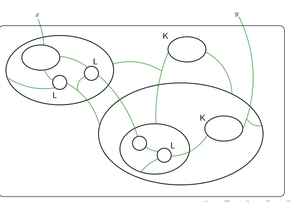
[image:7.363.35.334.49.256.2]x y
Figure 1: An example of a bigraph
1 Introduction
Bigraphical reactive systems (BRSs) [28, 29, 30, 20] are a graphical model of compu-tation in which bothlocalityandconnectivityare prominent. Recognising the increas-ingly topographical quality of global computing, they take up the challenge to base all distributed computation on graphical structure. A typical bigraph is shown in Figure 1. Such a graph is reconfigurable, and its nodes (the ovals and circles) may represent a great variety of computational objects: a physical location, an administrative region, a data constructor, aπ-calculus input guard, an ambient, a cryptographic key, a message, a replicator, and so on.
Bigraphs are a development of action calculi [26], but simpler. They use ideas from many sources: the Chemical Abstract machine (Cham) of Berry and Boudol [2], the π-calculus of Milner, Parrow and Walker [31], the interaction nets of Lafont [22], the mobile ambients of Cardelli and Gordon [7], the explicit fusions of Gardner and Wis-chik [16] developed from the fusion calculus of Parrow and Victor [33], Nomadic Pict by Wojciechowski and Sewell [41], and the uniform approach to a behavioural theory for reactive systems of Leifer and Milner [24]. This memorandum is self-contained; it builds on preliminary definitions and results put forward by Milner [29], but the approach here is a lot simpler and developed more fully.
The theory of BRSs responds to twin challenges: from application, and from exist-ing process theory. The former demands greater breadth of concepts, while the latter demands continuity of ideas. We now discuss these challenges separately.
A slightly more suggestive example
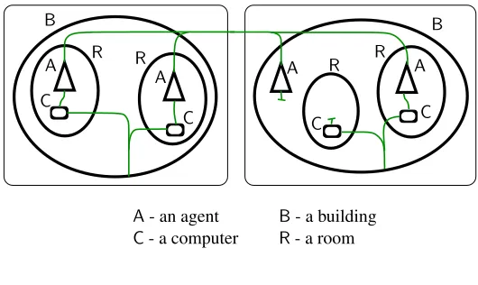
A C A A C A R R B B R R C CB- a building R- a room A- an agent
[image:8.363.49.314.72.230.2]C- a computer
Fig. 1. A bigraph for communication in a built environment
study typically remain stable —in so far as they are independent of human designs.
Our strategy here is to tackle just two aspects of mobile systems simultaneously:
mobile locality
and
mobile connectivity
. Already this combination presents a
chal-lenge: to what extent are locality and connectivity interdependent? In plain words,
does
where you are
affect
whom you can talk to
? The answer must lie in the level
of modelling. To a user of the Internet (seeing it abstractly) there is total
indepen-dence, and we want to model it at a high level, just as it appears to users. But to
the engineer these remote communications are not atomic; they involve chains of
interactions between neighbouring entities, and we must also provide a low-level
model which reflects this reality. These two levels must surely be part of a single
multi-level model that explains how higher levels are
realised
by lower levels.
Of the two levels, the lower is the less novel. Indeed, von Neumann’s cellular
au-tomata are the original paradigm for it; his agents were arranged on a fixed grid and
interaction could only occur between neighbours. But in such a concrete model we
hope to
realise
a higher level view in which a single agent is represented by
dif-ferent cells at difdif-ferent moments, and may send messages to other distant agents.
So the challenge we address here is to provide the means to view locality and
con-nectivity as dependently —or independently— as you wish, and to correlate these
views. This seems to require new mathematical structures, and bigraphs attempt to
provide them.
Example 1 (sentient buildings)
As a simple illustration, consider a crude version
of a
sentient built environment
, modelled as a bigraph in Figure 1. There are two
structures on the nodes of a bigraph; they may be nested, and they may also be
connected by links. The linkage is independent of the nesting, so links often cross
node boundaries. Nodes may be of many kinds, each represented by a
control
(
A, B,
. . .
) associated with each node. (The shape of nodes is suggestive but redundant.)
For this particular bigraph:
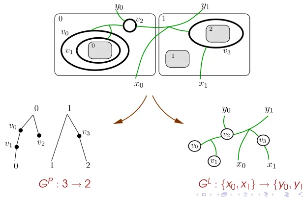
Pure bigraphs
G
:
h
3
,
{
x
0,
x1
}i → h
2
,
{
y
0,
y1
}i
Part II : Bigraphical structure
Section 5 defines the notion of aconcrete pure bigraphformally, in terms of its two con-stituents: aplace graphrepresenting locality and alink graphrepresenting connectivity. Sections 6 and 7 define these two notions in turn, ensuring that they enjoy the neces-sary categorical properties, including RPOs. Section 8 then combines these constituents, yielding a theory of pure bigraphs where locality and connectivity are independent. It defines important properties and operations for bigraphs; it also introduces a quotient functor from concrete toabstractbigraphs, where support is forgotten and the notions of occurrence and RPO are lost.
5 Pure bigraphs: definition
In this section we define the notion of
pure bigraph
formally, in terms of the
con-stituent notions of
place graph
and
link graph
, which are dealt with in the following
two sections. Let us begin with an illustration.
Example 4 (resolving a bigraph)
An example of a bigraph appeared in Figure 1;
it illustrated how nodes are nested, and how —independently of the nesting— they
are linked via their ports. Figure 3 shows another example, illustrating more of the
0 1 v1 v3 v0 v2 v2 v3 v0 v1 0 1 v0
v1 v2
v3 y0 y1 1 2 x0 x1 y0 y1 1 2 0
[image:9.363.38.346.58.259.2]0 x0 x1
Fig. 3. Resolving a bigraph into a place graph and a link graph
structure of bigraphs. First, it shows how a bigraph may be resolved into its two
constituents, a
place graph
and a
link graph
. This is what we mean by the
indepen-dence of placing and linking; the place graph (a forest) is completely independent
of the link graph (a kind of hypergraph) as long as they shared the same node set,
here
{
v
0, . . . , v
3}
. (Controls are not shown in this example.) If we forget everything
in the bigraph except the nesting of regions (large squares), nodes and sites (grey
G
P:
3
→
2
G
L:
{
x0
,
x1
} → {
y0
,
y1
}
Pure bigraphs, formally
[1]Definition (
SIGNATURE OF CONTROLSK
)
K
∈ K
has an
arity
ar
(
K
)
, its number of ports.
A control can be
atomic, and then not allowed to contain
further structure. Non-atomic controls can be
active
or
passive.
Definition (
PLACE GRAPH OVERK
)
G
P= (
V
,
ctrl
,
prnt
) :
m
→
n
with inner width (
sites
)
m
and outer
width (
roots
)
n
consisting of
a
control map
ctrl
:
V
→ K
; which assigns controls to nodes;
an acyclic
parent map
prnt
:
m
]
V
→
V
]
n
;
Pure bigraphs, formally
[2]Definition (
LINK GRAPH OVERK
)
G
L= (
V
,
E
,
ctrl
,
link
) :
X
→
Y
with inner names
X
and outer names
Y
consisting of
a
control map
ctrl
:
V
→ K
;
a finite set of
edges
E
;
a
link map
link
:
X
]
P
→
E
]
Y
mapping ‘
points
’ to ‘
links
’,
where
P
def=
P
v∈V
ar
(
ctrl
(
v
))
are called the
ports
of
G
L.
Terminology
A link is
idle
if it has no preimage under the link map;
open
if it is
an (outer) name;
closed
if it is an edge.
A link graph is
lean
if it has no idle edges.
Pure bigraphs, formally
[3]Definition (
PURE BIGRAPHS)
The
superimposition
of a place and a link graph sharing nodes
and control map. Namely,
G
= (
V
,
E
,
ctrl
,
prnt
,
link
) :
h
m
,
X
i → h
n
,
Y
i
where
G
P= (
V
,
ctrl
,
prnt
) :
m
→
n
is a place graph,
Bigraphs as a
(
⊗
,
◦
)
-algebra
H
=
G
◦
(
F
1⊗
F
2) :
→ h
1
,
{
x
,
y
}i
0#
2 2
1
2 5
0#
1
w z y x
2
x y
v
G
0# 2
2 5
0#
1
x y
H
5 5
0#
x y z v w
5 5
0#
1
2
F1 F2
F
1:
→ h
1
,
{
x
,
y
}i
F
2:
→ h
1
,
{
z
,
v
,
w
}i
F1⊗F2.
h
2
,
{
x
,
y
,
z
,
v
,
w
}i
G.
h
1
,
{
x
,
y
}i
Bigraphs as a
(
⊗
,
◦
)
-algebra
H
=
G
◦
(
F1
⊗
F
2) :
→ h
1
,
{
x
,
y
}i
0# 2 2 1 2 5 0# 1 w z y x 2 x y v G 0# 2 2 5 0# 1 x y H 5 5 0#
x y z v w
5 5
0#
1
2
F1 F2
0# 2 2 1 2 5 0# 1 w z y x 2 x y v G 0# 2 2 5 0# 1 x y H 5 5 0#
x y z v w
5 5
0#
1
2
F1 F2
F
1:
→ h
1
,
{
x
,
y
}i
F
2:
→ h
1
,
{
z
,
v
,
w
}i
F1⊗F2.
h
2
,
{
x
,
y
,
z
,
v
,
w
}i
G.
h
1
,
{
x
,
y
}i
Bigraphs as a
(
⊗
,
◦
)
-algebra
H
=
G
◦
(
F1
⊗
F
2) :
→ h
1
,
{
x
,
y
}i
0# 2 2 1 2 5 0# 1 w z y x 2 x y v G 0# 2 2 5 0# 1 x y H 5 5 0#
x y z v w
5 5
0#
1
2
F1 F2
0# 2 2 1 2 5 0# 1 w z y x 2 x y v G 0# 2 2 5 0# 1 x y H 5 5 0#
x y z v w
5 5
0#
1
2
F1 F2
F1
:
→ h
1
,
{
x
,
y
}i
F2
:
→ h
1
,
{
z
,
v
,
w
}i
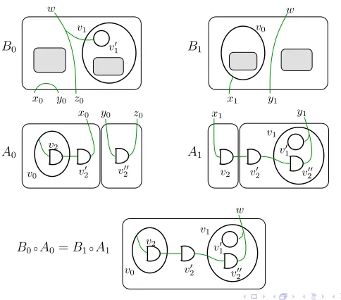
A second example of
(
⊗
,
◦
)
-composition
A1 B1 w A0 B0 w wB0◦A0=B1◦A1
v2 v02
v1 v0 v00 2 v0 1 v0 v2 v0
2 v002
v0 v2 v0 1 v1 v0 2 v0 1 v00 2 v1
x1 y1
y1
x1
y0 z0
x0
y0 z0
[image:19.363.65.307.46.259.2]x0
Figure 11: A consistent pairA~of bigraphs, with IPOB~
It can be shown that the members of(C~P, CP)have the same support as the mem-bers of(B~P,id). So we may form the triple of combinations
(hC0P, B0Li,hC1P, B1Li,hCP,idi)
(with suitable interfaces), and also prove it to be a candidate RPO in ´BIGforA~to ~
B. Hence there is a unique mediating arrow between the given RPO(B,~ id)and this candidate. The place graph constituent of this mediator then provides the required unique mediator in ´PLG, and we are done. A similar argument applies also to ´LIG. (⇐) Assuming IPOs in ´PLGand ´LIG, by routine diagram chasing we can verify the IPO property in ´BIG.
Example 9 (Bigraph IPOs) To illustrate IPOs in ´BIG, we can combine Example 7 for place graphs and Example 8 for link graphs, since they have the same node sets. In both cases the boundsB~are IPOs, and indeed pushouts because the graphsA~are epi.
The combination is shown in Figure 11. Again, both of the bigraphsA~are epi, so our results show that the boundB~is again an IPO and a pushout.
We now give a few special cases of IPOs. First, some pushouts (hence also IPOs) that are easy to verify for any precategory:
The s-category of pure bigraphs
Pure bigraphs are the arrows of a
s-category
´
B
IG(
K
).
They fail to be a category as both
◦
and
⊗
are partial.
Oh my!
◦
is partial because of the underlying concrete sets of
nodes
; s-categories make provisions in that respect.
⊗
is partial because of the sets of
names
; as names cannot
be taken up to iso, this is an intrinsic feature.
It is not so bad.
Abstract bigraphs
are the quotient classes of ‘
lean-support
’
equivalence
m
, where
G
m
H
if they are isomorphic after
discarding all
idle edges
.
B
IG(
K
)
is the
category
of abstract pure bigraphs, that is
The s-category of pure bigraphs
Pure bigraphs are the arrows of a
s-category
´
B
IG(
K
).
They fail to be a category as both
◦
and
⊗
are partial.
Oh my!
◦
is partial because of the underlying concrete sets of
nodes
; s-categories make provisions in that respect.
⊗
is partial because of the sets of
names
; as names cannot
be taken up to iso, this is an intrinsic feature.
It is not so bad.
Abstract bigraphs
are the quotient classes of ‘
lean-support
’
equivalence
m
, where
G
m
H
if they are isomorphic after
discarding all
idle edges
.
Merging roots and outer names in products
Two derived operators allow to merge outer names and roots
PARALLEL PRODUCT:
G
0k
G
1: like
⊗
with merge of outer
names;
It works by first making all the outer names disjoint, then
composing with
⊗
, and finally renaming names as originally
in the resulting bigraph.
PRIME PRODUCT:
G
0|
G
1: like
k
with merge of roots in the
Bigraphical term language
R. Milner 12
x K
a discrete ionK~x a closure/x a substitutiony/X
x0 xk−1 y
x0 xk−1
Fig. 11. Elementary linkings and ions
merge0 def
= 1
mergem+1 def
= join(id1⊗mergem).
Note thatmerge1=id1, and hencemerge2=join.
Alinkingorwiringis a bigraphX→Y, which necessarily has no nodes. All linkings can be expressed in terms of two kinds (see Figure 11):
/x : x→ closure
y/X : X→y substitutionx7→y(allx∈X).
A closure just closes a single link. ForX={x1, . . . , xk}we define the multiple closure /Xdef
=/x1⊗· · ·⊗/xk. ForX=X1]· · ·]XnandY ={y1, . . . , yn}, a multiple substitution σ:X→Y is defined byy1/X1⊗ · · · ⊗yn/Xn. A substitution need not be surjective. We writeY:→Y for the empty substitution (i.e. whenX is empty), or just y:→y if Y ={y}; these are the duals of closures. We shall useωto range over linkings,σ, τover substitutions, andα, βover the bijective substitutions, which we callrenamings.
Permutationsπ and renamings α, together with the identities, generate all isomor-phisms in the category of bigraphs; in fact every isomorphism takes the formπ⊗α. To see this, supposeι:I→J is an iso, with inverse κ. Since κι = idI and ικ = idJ the support ofιmust be empty, and its place graph and link graph must be bijections ιP:m→mandιL:X→Y, whereI=hm, XiandJ=hm, Yi. In other words,ι=hπ, αi
whereπis a permutation onmandαa renaming; this is readily expressed asι=π⊗α. The only other elementary bigraph is adiscrete ionK~x: 1→h1,{~x}i, for any sequence ~x=x0, . . . , xk−1of distinct names wherek=ar(K) (see Figure 11).
We now turn to the first of our normal forms. It depends on two important concepts:
Definition 4.2. (prime, discrete) An interface isprimeif it has unit width. It takes the formh1, Xi. A bigraphG:I→JisprimeifJis prime andIhas no names. A bigraph isdiscreteif every link joins exactly one point to an outer name.
This a discrete bigraph is open and has no idle names. A discrete ion is an instance of a prime discrete bigraph. More generally we define adiscrete moleculeM to be a prime discrete bigraph having a single outermost node.
The top part of Figure 12 shows a bigraphGand its underlying discrete bigraphD. Note thatDconsists just of discrete ions in a topographical arrangement; by composing it with a linking we recoverG.
Our proof of the existence of normal forms will use the following notions:
x y
x y x y
x/x
|
y/y
:
X
→
X
x y z w
/x
|
w/y
|
w/z
:
{
xyz
} →{
w
}
/z
◦(z/x
|
z/y) :
X
→
J
=
h
1
,
(
X
)
, X
i
,
I
=
h
1
,
(
∅
)
,
∅i
,
Interfaces:
xX
=
{
xy
}
.
yx
:
J
→
J
:
I
→
I
1 :
→
I
[image:27.363.29.349.41.261.2]y
Figure 7: Some simple bigraphs
Such ‘wide’ reaction rules are interesting in the presence of one or more active
controls, because they can be used to separate the components of a distributed redex
but still allow it to react. We have already introduced
amb
as an example of an active
control. Indeed, our categorical representation will allow us to insert a bigraph with
arbitrarily many global names in the double-width hole of the ambient rule’s redex.
In particular, we might insert an instance of the redex of our remote
π-calculus rule;
by this means we would create two interwoven but independent redexes, such that
neither reaction precludes the other. This is not an unlikely occurrence in the Internet,
modelled at a suitable level of abstraction.
In our illustrations of reaction rules we chose to stay close to familiar calculi.
Be-yond these, the possibilities range widely. For example, using a combination of active
and passive controls, various forms of
failure management
can be modelled. This may
include the inactivation of processes due to failure, the reporting of failures, recovery
procedures, and the subsequent re-activation of inactivated processes.
Our illustrations so far have emphasised dynamics. We should also realise that
some bigraphs have no dynamic behaviour but are useful building blocks. Figure 7
shows six simple examples, together with the terms that denote them. On the left side,
the first is just a region containing nothing. Its inner face is the so-called
origin
, the
simplest possible interface where everything is null, while its outer face is the simplest
interface
I
of width
1
. The second is the categorical identity at
I. The third is again an
identity at an interface
J
of width
1
, but here the site has two local names.
The three bigraphs on the right side of the figure will be called
wirings; they have
both interfaces of width
0
, i.e. of the form
h
0
,
()
, X
i
, which we abbreviate to
X
(a set
of names). Their function is to link
global
inner and outer names in various patterns.
The first wiring is just the identity on an interface
{
xy
}
; think of it as the identity
substitution
on these two names. The next involves a substitution of the name
w
for
both the inner names
y
and
z. This wiring also
closes
the inner name
x; that is, when
composed with another bigraph with name
x, such as
R
in Example 3, it will remove
x
from the outer face. The last is an example of what Gardner and Wischik [16] call a
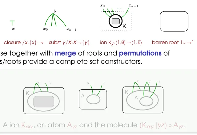
closure/x:{x}→ substy/X:X→{y} ion K~x:h1,∅i→h1,~xi barren root 1:→1
These together with
merge
of roots and
permutations
of
sites/roots provide a complete set constructors.
A A
x
K
x
the ionKxxy
K
the atomAyz the moleculeKxxy.Ayz
y z y z
y
The diagram shows a molecule built from an ion and an atom, in such a way that the ion and atom share a name. The possibility for nested nodes to share a name at different levels is important; our chosen notationK~x.Palso agrees with the notation
for prefixing in CCS andπ-calculus. We shall see a close semantic correspondence in Section 11.
Let us now considerdiscretebigraphs. In a precise sense they complement wiring:
Proposition 8.15 (discrete normal form) Every bigraphG:hm, Xi →hn, Zican be expressed uniquely, up to a link iso onY, asG= (idn⊗ω)D, whereω:Y→Z
is a wiring andD:hm, Xi →hn, Yiis discrete. Furthermore every such discrete
Dmay be factored uniquely, up to a place iso on the domain of each factorDi, as
D=α⊗((D0⊗ · · · ⊗Dn−1)ι)
withαa renaming, eachDiprime and discrete, andιa permutation of sites.
Note that a renaming is discrete but not prime (since it has zero width); this explains
αin the prime factorisation. Its uniqueness depends on the fact that primes have no inner names. In the special case thatDis ground, the factorisation is justD = d0⊗ · · · ⊗dn−1, a product of prime discrete ground bigraphs.
Thediscrete normal form (DNF)applies equally to abstract bigraphs, and plays an important part in the complete axiomatisation of pure bigraphs [37]. Discreteness is well behaved in other ways. Clearly both composition and tensor product preserve it. IPOs also treat it well. In fact, we have:
Proposition 8.16 (properties of discreteness) The discrete pure bigraphs form a sub-s-category of ´BIGh. Moreover
(1) IfDis discrete and(D0, G0)is an IPO for(G, D), thenD0is discrete. (2) IfD, D0are discrete and(D0,id
n⊗ω)bounds(G, D), then it is a pushout.
We have to make one more preparation for Section 9 on dynamics. When we define the notion of parametric reaction rule, we must allow a parametric redex to replicate some factors of its parameter and discard other factors. For example, the redexR
for CCS shown in Figure 2 discards two of the four factors. We represent this by an operationη[·]on parameters calledinstantiation. The following definition ensures
41
A ion
K
xxy, an atom
A
yzand the molecule
(
K
xxyk
yz
)
◦
A
yz.
Bigraphical term language
R. Milner 12
x K
a discrete ionK~x a closure/x a substitutiony/X
x0 xk−1 y
x0 xk−1
Fig. 11. Elementary linkings and ions
merge0 def
= 1
mergem+1 def
= join(id1⊗mergem).
Note thatmerge1=id1, and hencemerge2=join.
Alinkingorwiringis a bigraphX→Y, which necessarily has no nodes. All linkings can be expressed in terms of two kinds (see Figure 11):
/x : x→ closure
y/X : X→y substitutionx7→y(allx∈X).
A closure just closes a single link. ForX={x1, . . . , xk}we define the multiple closure /Xdef
=/x1⊗· · ·⊗/xk. ForX=X1]· · ·]XnandY ={y1, . . . , yn}, a multiple substitution σ:X→Y is defined byy1/X1⊗ · · · ⊗yn/Xn. A substitution need not be surjective. We writeY:→Y for the empty substitution (i.e. whenX is empty), or just y:→y if Y ={y}; these are the duals of closures. We shall useωto range over linkings,σ, τover substitutions, andα, βover the bijective substitutions, which we callrenamings.
Permutationsπ and renamings α, together with the identities, generate all isomor-phisms in the category of bigraphs; in fact every isomorphism takes the formπ⊗α. To see this, supposeι:I→J is an iso, with inverse κ. Since κι = idI and ικ = idJ the support ofιmust be empty, and its place graph and link graph must be bijections ιP:m→mandιL:X→Y, whereI=hm, XiandJ=hm, Yi. In other words,ι=hπ, αi
whereπis a permutation onmandαa renaming; this is readily expressed asι=π⊗α. The only other elementary bigraph is adiscrete ionK~x: 1→h1,{~x}i, for any sequence ~x=x0, . . . , xk−1of distinct names wherek=ar(K) (see Figure 11).
We now turn to the first of our normal forms. It depends on two important concepts:
Definition 4.2. (prime, discrete) An interface isprimeif it has unit width. It takes the formh1, Xi. A bigraphG:I→JisprimeifJis prime andIhas no names. A bigraph isdiscreteif every link joins exactly one point to an outer name.
This a discrete bigraph is open and has no idle names. A discrete ion is an instance of a prime discrete bigraph. More generally we define adiscrete moleculeM to be a prime discrete bigraph having a single outermost node.
The top part of Figure 12 shows a bigraphGand its underlying discrete bigraphD. Note thatDconsists just of discrete ions in a topographical arrangement; by composing it with a linking we recoverG.
Our proof of the existence of normal forms will use the following notions:
x y
x y x y
x/x
|
y/y
:
X
→
X
x y z w
/x
|
w/y
|
w/z
:
{
xyz
} →{
w
}
/z
◦(z/x
|
z/y) :
X
→
J
=
h
1
,
(
X
)
, X
i
,
I
=
h
1
,
(
∅
)
,
∅i
,
Interfaces:
xX
=
{
xy
}
.
yx
:
J
→
J
:
I
→
I
1 :
→
I
[image:28.363.13.363.44.263.2]y
Figure 7: Some simple bigraphs
Such ‘wide’ reaction rules are interesting in the presence of one or more active
controls, because they can be used to separate the components of a distributed redex
but still allow it to react. We have already introduced
amb
as an example of an active
control. Indeed, our categorical representation will allow us to insert a bigraph with
arbitrarily many global names in the double-width hole of the ambient rule’s redex.
In particular, we might insert an instance of the redex of our remote
π-calculus rule;
by this means we would create two interwoven but independent redexes, such that
neither reaction precludes the other. This is not an unlikely occurrence in the Internet,
modelled at a suitable level of abstraction.
In our illustrations of reaction rules we chose to stay close to familiar calculi.
Be-yond these, the possibilities range widely. For example, using a combination of active
and passive controls, various forms of
failure management
can be modelled. This may
include the inactivation of processes due to failure, the reporting of failures, recovery
procedures, and the subsequent re-activation of inactivated processes.
Our illustrations so far have emphasised dynamics. We should also realise that
some bigraphs have no dynamic behaviour but are useful building blocks. Figure 7
shows six simple examples, together with the terms that denote them. On the left side,
the first is just a region containing nothing. Its inner face is the so-called
origin
, the
simplest possible interface where everything is null, while its outer face is the simplest
interface
I
of width
1
. The second is the categorical identity at
I. The third is again an
identity at an interface
J
of width
1
, but here the site has two local names.
The three bigraphs on the right side of the figure will be called
wirings; they have
both interfaces of width
0
, i.e. of the form
h
0
,
()
, X
i
, which we abbreviate to
X
(a set
of names). Their function is to link
global
inner and outer names in various patterns.
The first wiring is just the identity on an interface
{
xy
}
; think of it as the identity
substitution
on these two names. The next involves a substitution of the name
w
for
both the inner names
y
and
z. This wiring also
closes
the inner name
x; that is, when
composed with another bigraph with name
x, such as
R
in Example 3, it will remove
x
from the outer face. The last is an example of what Gardner and Wischik [16] call a
closure/x:{x}→ substy/X:X→{y} ion K~x:h1,∅i→h1,~xi barren root 1:→1
These together with
merge
of roots and
permutations
of
sites/roots provide a complete set constructors.
A A
x
K
x
the ionKxxy
K
the atomAyz the moleculeKxxy.Ayz
y z y z
y
The diagram shows a molecule built from an ion and an atom, in such a way that the ion and atom share a name. The possibility for nested nodes to share a name at different levels is important; our chosen notationK~x.Palso agrees with the notation
for prefixing in CCS andπ-calculus. We shall see a close semantic correspondence in Section 11.
Let us now considerdiscretebigraphs. In a precise sense they complement wiring:
Proposition 8.15 (discrete normal form) Every bigraphG:hm, Xi →hn, Zican be expressed uniquely, up to a link iso onY, asG= (idn⊗ω)D, whereω:Y→Z
is a wiring andD:hm, Xi →hn, Yiis discrete. Furthermore every such discrete Dmay be factored uniquely, up to a place iso on the domain of each factorDi, as
D=α⊗((D0⊗ · · · ⊗Dn−1)ι)
withαa renaming, eachDiprime and discrete, andιa permutation of sites.
Note that a renaming is discrete but not prime (since it has zero width); this explains
αin the prime factorisation. Its uniqueness depends on the fact that primes have no inner names. In the special case thatDis ground, the factorisation is justD =
d0⊗ · · · ⊗dn−1, a product of prime discrete ground bigraphs.
Thediscrete normal form (DNF)applies equally to abstract bigraphs, and plays an important part in the complete axiomatisation of pure bigraphs [37]. Discreteness is well behaved in other ways. Clearly both composition and tensor product preserve it. IPOs also treat it well. In fact, we have:
Proposition 8.16 (properties of discreteness) The discrete pure bigraphs form a sub-s-category of ´BIGh. Moreover
(1) IfDis discrete and(D0, G0)is an IPO for(G, D), thenD0is discrete.
(2) IfD, D0are discrete and(D0,idn⊗ω)bounds(G, D), then it is a pushout.
We have to make one more preparation for Section 9 on dynamics. When we define the notion of parametric reaction rule, we must allow a parametric redex to replicate some factors of its parameter and discard other factors. For example, the redexR
for CCS shown in Figure 2 discards two of the four factors. We represent this by an operationη[·]on parameters calledinstantiation. The following definition ensures
41
A ion
Kxxy
, an atom
Ayz
and the molecule
(
Kxxy
k
yz
)
◦
Ayz
.
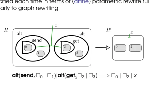
Bigraphical reactive systems, CCS
The
dynamics
of bigraphs is not hardwired in the model, but
specified each time in terms of (
affine
) parametric rewrite rules.
Similarly to graph rewriting.
x x
alt
alt
R
R
0 [image:29.363.33.331.64.252.2]0 1 2 3 2 0
get
send
Fig. 2. A bigraphical reaction rule for CCS with summation
thus admitting more refined applications. It will be seen that the basic theory of
pure bigraphs is preserved by these specialisations, thus establishing pure bigraphs
as a core theory.
However, the theory cannot claim to be definitive; many variations are possible.
Therefore this work has been divided as much as possible into separate topics,
making it more amenable to variation. For example,
bigraphs
themselves are
de-fined in terms of two independent structures,
place graphs
and
link graphs
, and
each of these can be varied. Also,
bigraphical reactive systems
(Brss) are defined
as merely one instance of a general concept,
wide reactive systems
(Wrss), whose
abstract theory we develop in Part I; many other instances are possible.
We now introduce our running example.
Example 2 (reaction in CCS)
The calculus CCS [30] has a reaction rule
(
x.P
+
M
)
|
(
x.Q
+
N
)
−→
P
|
Q ,
where
x.P
and
x.Q
are guarded output and input respectively, while
M
and
N
represent zero or more alternatives of the same nature. The rule represents a
com-munication on channel
x
, which may preempt other possible communicators on the
same channel; the result of the communication is to allow the continuations
P
and
Q
to continue in parallel, while the alternatives
M
and
N
are discarded.
Figure 2 shows the corresponding reaction rule in bigraphs. It uses three controls:
send
for output,
get
for input and
alt
for alternation. They are declared to be
passive
controls, i.e. no reaction can occur inside them. The reaction rule means that the
redex
R
occurring in a larger bigraph, with anything in its holes (grey boxes), can
be replaced by the
reactum
R
0, retaining some of the contents of
R
as indicated by
the ordinals in its holes. Note several points:
•
The
send
- and
get
- nodes are connected in
R
by a link named
x
. In the larger
con-text these may be linked to competitors for communication on that link. Nothing
in
R
0retains that link, but competitors in the larger context will retain it.
•
The occupants of the holes —collectively called the
parameter
of the reaction—
may freely be linked to the larger context (and to each other); they may even
contain uses of the link
x
, which may later be activated.
alt
(
send
x0|
1)
|
alt
(
get
x2|
3)
.
0|
2|
x
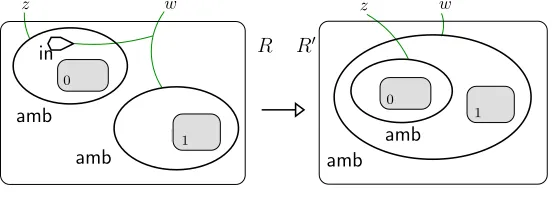
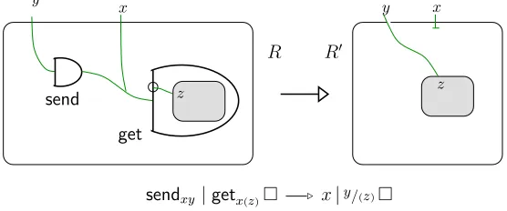
Bigraphical reactive systems, Ambients
sum
sum
x y
R
R
0x y
z z
send
get
sum
(
send
xy0|
1)
|
sum
(
get
x(z)2|
3)
.x
|
0|
y/(z)22 0
1 3
2 0
Figure 4: A reaction rule for theπ-calculus with summation
0
amb
amb
1
in
amb
0
1
amb
R
0R
amb
z(
in
w|
0)
|
amb
w1 .amb
w(
amb
z0|
1)
w z
[image:30.363.45.321.78.188.2]z w
Figure 5: Reaction rule for the ambient calculus
Bigraphical reactive systems, Petri nets
r
x1 y1 y2 x1 y1 y2
[image:31.363.37.324.91.211.2]r′
Figure 12: A link-graph reaction rule for condition-event nets
Then the concrete precategory of many-one sorted condition-event nets is
´CE =def ´LIG(Σpetri)
and we denote its lean-support quotient by CE. Although these nets share many-one sorting with arithmetic nets, there is a considerable difference; this arises from the fact that in arithmetic nets every node possesses exactly ones-port, while in ´CE the event nodes have none. This illustrates the versatility of many-one sorting.
In general an interface may contain boths-names andt-names. But in the example bothxandyares-names, because each is a link containing a condition. So let us define ans-interface to be one containing onlys-names; then we can model condition-event nets in ´CE and CE as link graphs withs-interfaces, and call thems-nets.
Without further ado we now set up in ´CE a raw transition systemLp, whose
inter-faces ares-interfaces and whose transitionsa ℓ ⊲bare those we have already described withℓ= +x,−xorτ. We also close the transitions under support equivalence. This induces a TS[[Lp]]in CE. Let us use∼pfor the associated bisimilarity in both cases.
Since no RPO theory is involved, we readily find
Proposition 9.1 (raw bisimilarity)
1. a ℓ ⊲a′in ´CE iff[[a]] ℓ ⊲[[a′]]in CE.
2. a∼pbin ´CE iff[[a]]∼p[[b]]in CE.
To compare this raw TS and bisimilarity with a contextual one, we must add reac-tion rules to ´CE, to make it an LRS. To match the firing rule, for each pairh, kwe introduce a reaction rule forEhk as illustrated in Figure 12 forh = 1, k = 2. As
re-quired by Definitions 4.2 and 7.1, we close this set under support translation and make each rule lean (no idle edges). Having thus established ´CE as a concrete LRS, we equip it with the standard transition system ST. We can then apply Corollary 7.2 to establish that the associated bisimilarity∼g, is a congruence.
Now we wish to refine the transition system in two steps. The first step is to reduce its transitions to the engaged ones.
Proposition 9.2 (adequacy for nets) The engaged transition system ETover ´CE is definite and adequate forST; therefore its bisimilarity coincides with∼g.
M
x1|
E
x1,y1y2|
U
y1|
U
y2.
U
x1|
E
x1,y1y2|
M
y1|
M
y2Bigraphical reactive systems, formally
A
parametric reaction rule
has a
redex
R
and a
reactum
R
0, and
takes the following form
(
R
:
I
→
J
,
R
0:
I
0→
J
, %
)
,
where
%
maps sites of
R
0back to
R
injectively.
For
d
a tuple of parameters, this results in a ground reaction rule
(
id
X⊗
R
)
◦
d
,
(
id
X⊗
R
0)
◦
%
(
d
)
Disclaimer (
BASIC BIGRAPHICAL REACTIVE SYSTEMS)
They enforce important simplifying properties of redexes:
flatness
Bigraphical reactive systems, formally
A
parametric reaction rule
has a
redex
R
and a
reactum
R
0, and
takes the following form
(
R
:
I
→
J
,
R
0:
I
0→
J
, %
)
,
where
%
maps sites of
R
0back to
R
injectively.
For
d
a tuple of parameters, this results in a ground reaction rule
(
id
X⊗
R
)
◦
d
,
(
id
X⊗
R
0)
◦
%
(
d
)
Disclaimer (
BASIC BIGRAPHICAL REACTIVE SYSTEMS)
They enforce important simplifying properties of redexes:
flatness
The essence of bigraphical reactive systems
For a ground prime term
a
and a ground reaction rule
(
r
,
r
0)
, we
derive a
standard
transition
a
L.
a
0as below, where
L
and
D
are an
idem pushout
of
a
and
r
and
D
is an
active
context.
L
a
r r!
a! D
We write
∼
STfor the
bisimilarity
of the
standard transition system
.
We then focus on
engaged transitions
, where the agent shares
at least one node with the parametric redex
R
underlying
r
. Let
∼
FPEbe the associated bisimilarity.
Theorem
Binding bigraphs
An important element is still missing in the model:
the possibility of making a name
local.
L
K
L L
K
x y
Figure 1: An example of a bigraph
1 Introduction
Bigraphical reactive systems (BRSs) [28, 29, 30, 20] are a graphical model of compu-tation in which bothlocalityandconnectivityare prominent. Recognising the increas-ingly topographical quality of global computing, they take up the challenge to base all distributed computation on graphical structure. A typical bigraph is shown in Figure 1. Such a graph is reconfigurable, and its nodes (the ovals and circles) may represent a great variety of computational objects: a physical location, an administrative region, a data constructor, aπ-calculus input guard, an ambient, a cryptographic key, a message, a replicator, and so on.
Bigraphs are a development of action calculi [26], but simpler. They use ideas from many sources: the Chemical Abstract machine (Cham) of Berry and Boudol [2], the π-calculus of Milner, Parrow and Walker [31], the interaction nets of Lafont [22], the mobile ambients of Cardelli and Gordon [7], the explicit fusions of Gardner and Wis-chik [16] developed from the fusion calculus of Parrow and Victor [33], Nomadic Pict by Wojciechowski and Sewell [41], and the uniform approach to a behavioural theory for reactive systems of Leifer and Milner [24]. This memorandum is self-contained; it builds on preliminary definitions and results put forward by Milner [29], but the approach here is a lot simpler and developed more fully.
The theory of BRSs responds to twin challenges: from application, and from exist-ing process theory. The former demands greater breadth of concepts, while the latter demands continuity of ideas. We now discuss these challenges separately.
Observe the difference between
closure
/
x
, where an edge
‘solidifies’
once and for all, and the concept that an edge is
available only within certain confines. Reminiscent of
communication in
ambient calculus
.
Binding bigraphs
An important element is still missing in the model:
the possibility of making a name
local.
L
K
L L
K
x y
Figure 1: An example of a bigraph
1 Introduction
Bigraphical reactive systems (BRSs) [28, 29, 30, 20] are a graphical model of compu-tation in which bothlocalityandconnectivityare prominent. Recognising the increas-ingly topographical quality of global computing, they take up the challenge to base all distributed computation on graphical structure. A typical bigraph is shown in Figure 1. Such a graph is reconfigurable, and its nodes (the ovals and circles) may represent a great variety of computational objects: a physical location, an administrative region, a data constructor, aπ-calculus input guard, an ambient, a cryptographic key, a message, a replicator, and so on.
Bigraphs are a development of action calculi [26], but simpler. They use ideas from many sources: the Chemical Abstract machine (Cham) of Berry and Boudol [2], the
π-calculus of Milner, Parrow and Walker [31], the interaction nets of Lafont [22], the mobile ambients of Cardelli and Gordon [7], the explicit fusions of Gardner and Wis-chik [16] developed from the fusion calculus of Parrow and Victor [33], Nomadic Pict by Wojciechowski and Sewell [41], and the uniform approach to a behavioural theory for reactive systems of Leifer and Milner [24]. This memorandum is self-contained; it builds on preliminary definitions and results put forward by Milner [29], but the approach here is a lot simpler and developed more fully.
The theory of BRSs responds to twin challenges: from application, and from exist-ing process theory. The former demands greater breadth of concepts, while the latter demands continuity of ideas. We now discuss these challenges separately.
Observe the difference between
closure
/
x
, where an edge
‘solidifies’
once and for all, and the concept that an edge is
available only within certain confines. Reminiscent of
communication in
ambient calculus
.
A binding bigraph
Typed Polyadic Pi-calculus in Bigraphs
∗
Mikkel Bundgaard
IT University of Copenhagen
Vladimiro Sassone
ECS, University of Southampton
Abstract
Bigraphs have been introduced with the aim to provide a topo-graphical meta-model for mobile, distributed agents that can ma-nipulate their own communication links and nested locations. In this paper we examine a presentation of type systems on bigraphical systems using the notion of sorting. We focus our attention on the typed polyadicπ-calculus with capability types `a la Pierce and San-giorgi, which we represent using a novel kind of link sorting called subsorting. Using the theory of relative pushouts we derive a la-belled transition system which yield a coinductive characterisation of a behavioural congruence for the calculus. The results obtained in this paper constitute a promising foundation for the presentation of various type systems for the (polyadic)π-calculus as sortings in the setting of bigraphs.
Categories and Subject Descriptors F.3.2 [Logics and Meanings of Programs]: Semantics of Programming Languages—Process models
General Terms Languages, Theory.
Keywords Bigraphs, typed polyadicπ-calculus, sortings, subsort-ing, bisimulation congruences, relative pushouts.
Introduction
Bigraphical reactive systems (BRS) [8] have been proposed as a topographical meta-model for mobile, distributed agents that can manipulate their own communication linkage and nested locations. Bigraphs generalise both the link structure characteristic of theπ -calculus and the nested location structure characteristic of the cal-culus of Mobile Ambients. A bigraph consists of two overlapping structures: a place graph and a link graph. The place graph is a tu-ple of unordered trees that represents the topology of the system. Its roots contain nodes which represent locations or process construc-tors. Some of the leaves may be sites to be filled by other bigraphs, so giving rise to bigraphical (multi-hole) contexts. Each node is typed with a control which prescribes its number of ports. The link graph represents the system’s connectivity. It links together ports and names in the bigraph’s inner and outer interfaces. Names in the inner interface represent connection points offered to bigraphs
∗Supported by ‘DisCo: Semantic Foundations of Distributed Computation,’
EU IHP ‘Marie Curie’ HPMT-CT-2001-00290.
Permission to make digital or hard copies of all or part of this work for personal or classroom use is granted without fee provided that copies are not made or distributed for profit or commercial advantage and that copies bear this notice and the full citation on the first page. To copy otherwise, to republish, to post on servers or to redistribute to lists, requires prior specific permission and/or a fee.
that may fill sites; those in the outer interface represent free names exported by the system.
Binding bigraphs extend this basic structure – known as pure bigraphs – by allowing some of the ports of a node to be ‘bind-ing,’ meaning that all other points linked to the port must lie inside the node. A binding port enforces a notion of scope on a bigraph’s links, resembling in such a way the usual notion of binders in theλ -and theπ-calculus. Binding interfaces record topological informa-tion (viz., sites and roots), inner and outer namesets, as well as the binding of names to locations. Fig. 1 depicts a binding bigraph with inner interfaceh3,({x2},∅,∅),{x0,x1,x2}i, reflecting that it consists
of three sites (shaded in the picture) only the first of which con-tains a local name, the binder x2. The bigraph’s outer interface is
h2,(∅,∅),{y0,y1,y2}i, with two roots, or locations (drawn in dashed
lines), and only global names.
r0
y0 y1
v0 v4 v2 s0 x2 v5 r1 y2 x1 x0 v1 s2 s1
Figure 1. A binding bigraph
Often when representing systems and calculi as bigraphical re-active systems one needs to constrain the allowable compositions of nodes and links. Examples of such constraints are Jensen’s rep-resentation of theπ-calculus with guarded sum [6], where for in-stance nodes of a given controlsummust not contain nodes of the same control as immediate children, or Leifer and Milner’s treat-ment of Petri nets [13], where transitions can only be connected to places and vice versa. A sorting is used to enforce constraints such as these on a class of bigraphs.
The polyadicπ-calculus [14] is a generalisation of the monadic
π-calculus, whereby a single message can carry a tuple of names rather than a single one. This has the immediate consequence that communication can go ‘wrong’ in that communicating parties may not agree on the number of names exchanged in a communication. A type system is needed to ensure that only well-formed processes are allowed by the formalism. In his original presentation of the polyadicπ-calculus in [14], Milner introduced a simple sorting dis-cipline to ensure ‘arity’ safety of communications. Pierce and San-giorgi presented in [17] a generalisation of Milner’s sorting with capability types and a structural subtype relation on sorts, which in addition can ensure that well-typed processes use names only for input (resp. output) actions, according to a predefined discipline. Inspired by this work and following Jensen and Milner’s encoding
π