Real-Time Path-Planning Optimisation Algorithm for Obstacle Avoidance
S. -H. Hur and L. Petropoulakis
Department of Electronic and Electrical Engineering, University of Strathclyde,
50 George Street, Glasgow G1 1QE, U.K e:[email protected]
This paper presents a new real-time path planning algorithm suitable for implementation on small mobile robots to aid navigation in unknown environments. The Random Obstacle Avoidance (R.O.A) algorithm was developed for small robots and it can be used as the basis for mapping the environment. The algorithm has been tested through a specially developed simulation environment using MATLAB. The main characteristics of the algorithm are simplicity, ease of implementation, speed, and efficiency.
Copyright © 2006 USTRATH
Keywords: path planning, obstacle avoidance, mobile robot control.
1. INTRODUCTION
Obstacle Avoidance algorithms generally enable autonomous vehicles to navigate without colliding with obstacles and are generally classified as those employed in known environments and those used in unknown environments. Many algorithms exist for known environments. These include Visibility Graph Representation, Configuration Space Method, Voronoi Diagrams, Dijkstra’s Shortest Path Algorithm and Minkowski Sum. These algorithms are generally used alongside path smoothing methods such as the Cubic Splines or the Post Processing method. This is required as obstacle avoidance algorithms do not normally account for the physical limitations of the robot or the constraints of the paths to be followed
Clearly, it is far more complex to develop algorithms for use in unknown or semi-structured environments. This paper suggests one such algorithm which may be used in real-time for small robots to:
a) Avoid randomly appearing unknown obstacles in the path of a robot and
b) Return the robot to an assumed optimal path towards a goal. For known or semi-structured environments this path is pre-evaluated using procedures not outlined in this paper.
The common uses of path-planning algorithms are in robot navigation (Ringdahl, 2003) and flight formation (Ousingsawat, 2004) amongst others.
In this case it was intended that the algorithm be kept as simple as possible for ease of implementation and due to hardware limitations associated with small mobiles. Thus, substantial problem simplification was assumed, including working on just first integrals and relying heavily on sensory inputs. Hence, despite apparent connections to other path-planning systems, no direct comparisons can be drawn here given their complexity.
In this paper, the basic navigational concepts are described in section 2. Section 3 introduces the ROA algorithm which uses Cardinal Splines for providing smooth motion. Section 4 exemplifies the operation of the algorithm in the presence of unknown obstacles. The navigation is simulated in MATLAB, through a specially developed Graphic User Interface (GUI). Conclusions are in section 5, followed by references.
2. BASIC NAVIGATIONAL CONCEPTS
First we define the orientation, the steering angle, and the heading of the robot.
The orientation
φ
of the robot is defined as the angle that the central longitudinal axis of the robot makes with the x-axis (fig.2).At any moment in time t, the steering angleα is by the difference in the robot orientation at time t and t-1.
The heading
θ
is defined as the angle that the line, connecting the central front point of the robot and the target, makes with the x-axis as shown in fig. 2. The robot shown in fig. 1 is therefore considered to be at ‘0’ or ‘initial’ orientation. [image:2.595.312.537.131.403.2]Fig. 1. Structure of simulated robot
Fig. 2. Heading and orientation
Fig. 3. Turning Radius
L is the length between the front and centre markers of the robot (fig.3) and given as:
2 2
2
)
(
)
(
x
fx
cy
fy
cL
=
−
+
−
(1)where (xc, yc) and (xf, yf) are centre and front
coordinates respectively.
∂ is defined in (fig. 3) as:
2
2
α
π
−
=
∂
(2),where
α
is the steering angle and the radius of the turning circle, r, is (fig. 3):∂
=
cos
L
r
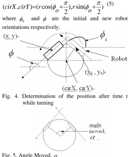
(3)With the radius of the turning circle, r, known, the centre coordinates of the turning circle, (cirX, cirY) (fig. 4) are derived as:
(
,
) ( cos(
), sin(
2
2
cirX cirY
r
r
o
o
)
π
π
φ
φ
=
+
+
(5)where φ0 and φ are the initial and new robot orientations respectively.
Fig. 4. Determination of the position after time t ile turning
wh
Fig. 5. Angle Moved, α
Assuming a constant speed the distance, d, traversed by the robot is d =vt, where v is the velocity and t is the time interval. Now, if c is the circumference of circle then we can easily derive:
π α
2
=
c
d (6)
By using the aforementioned equations, we can now calculate the position of the robot after a time, t, either when the steering angle,
α
, is zero, i.e. going straight, or the steering angle is non-zero, i.e. turning as follows (Ringdahl, 2003):If α= 0, i.e. zero steering •
φ
=φ
o •0 c o s ( )
x = x + d
φ
•
0 s i n ( )
y = y + d
φ
,where x , y and x0, yo are new and initial x and y
coordinates of the robot respectively.
If α ≠0, i.e. non-zero steering angle (fig. 4) •
φ
=φ
0+α
• )
2 cos(φ+π −
=cirX r
x
• )
2 sin(φ+π −
=cirY r
y
where r is the radius of the turning circle and, φ0 and
[image:2.595.63.256.235.587.2]The rotational matrix,
⎥ ⎦ ⎤ ⎢ ⎣ ⎡ ⎥ ⎦ ⎤ ⎢
⎣
⎡ −
= ⎟⎟ ⎠ ⎞ ⎜⎜ ⎝ ⎛
yy xx Y
X
φ φ
φ φ
cos sin
sin
cos (7)
is used during simulation to evaluate and then plot the robot position and orientation.
[image:3.595.67.268.237.345.2]In equation (7), xx and yy are the respective x and y coordinates of the robot at 0 orientation and X and are the x and y coordinates at orientation
φ
.Fig. 6 illustrates the robot approaching an obstacle and four stars (a, b, c, d) representing the assumed sensing actions that identify obstacles and provide a safety margin.
Fig. 6. Robot with sensing system approaching an stacle
ob
The following equations are used to calculate the heading of the robot with obstacles, walls or goal. For a positive heading angle,
)
(
cos
1l
x
±
=
−θ
(8),where x is the x-coordinate of the obstacle, wall or goal minus the x-coordinate of the centre of robot and l is the length between the centre of robot and the obstacle, wall or goal. For a negative heading angle,
)
(
cos
360
1l
x
±
−
=
−θ
(9)In real life, the robot takes appropriate action when it detects any obstacles within its safety margin, i.e. when the distance between robot and the obstacle is less than the distance between the robot and any of the action sensing points, (fig. 6). For simulation purposes, obstacles are assumed to be encircled rectangular objects (the circle being of defined radius), and the robot has to continuously calculate the distances between the sensing points and the centre point of an obstacle. Hence if a distance between any of the sensing points and the centre of an obstacle becomes shorter than the radius of the circle surrounding the obstacle, the robot knows that a part of the obstacle is likely to be within the safety margin and takes action to avoid the obstacle. Walls enclosing the simulated area are approximated as straight line obstacles (or arcs of very large circles).
For simulation purposes it is also assumed that use of additional sensors results in better accuracy. However, too many simulated sensors slow down the simulation as the distances between the robot and the obstacles are evaluated constantly.
3. RANDOM OBSTACLE AVOIDANCE (ROA) ALGORITHM
The ROA algorithm uses the basic concept of Cardinal Spline as defined in (IBM Corporation) and (Twigg, 2003). The following steps explain how the algorithm works:
Step 1 Assuming there are no random or unknown obstacles present, we find the optimal path from the source to the goal, i.e. straight line from the source to the goal if the environment is fully unknown. Note that in the case of partially known environments, this will not be a straight line (fig. 16).
Step 2 While following the predefined path obtained from step 1, if there are any random obstacles present, turn right or left to clear the obstacle from the sensors. The robot determines whether to turn right or left based on the following process (with respect to the robot shown in fig. 6):
For simple binary sensors a, b, c and d
If (a is on OR b is on) AND (c is off AND d is off) - Then: Turn right (negative steering angle) If (a is on AND b is off) AND (c is on AND d is off) - Then: Turn right
If (a is on AND b is on) AND (c is on AND d is off) - Then: Turn right
ELSE
- Turn left (positive steering angle)
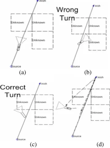
Using this approach it can be seen that in fig. 7, that the robot encounters an obstacle with sensors a or b on (fig. 7(a)), and turns right only to collide with another obstacle (fig. 7(b)). A simple modification of the algorithm, so that “while turning to clear an obstacle, if another obstacle is detected, there must be a change in the sign of the steering angle”, solves the problem as shown in fig. 7(c). Robot moves from fig. 7(a) to 7(c) and finally to 7(d) in the modified case.
(a) (b)
[image:3.595.317.496.530.770.2]Step 3 When the robot has cleared an obstacle it generates a new path using the Cardinal Spline (fig. 8) to get the robot back on track towards the goal. The spline is created using the following control points:
[image:4.595.325.524.79.148.2][Centre coordinates, Centre coordinates, Sensing point, Look Ahead Point, Goal, Goal].
Fig. 8. Cardinal Spline
This sequence of control points is due to the Cardinal Spline implementation (Twigg, 2003). For example, if A, B, C and D are the control points (fig. 8) then the segment starts at B and ends at C. The points A and D are present only to define the shape of the line segmentBC. Therefore, the segment AB is drawn with the control points A, A, B and C, BC is drawn with the control points A, B, C and D, and so on. Hence, to obtain the spline shown in fig. 8, the set of control points must be A, A, B, C, D, E, E.
[image:4.595.65.237.133.199.2]Our algorithm uses a Look Ahead Point (LAP), described in step 4, as one of the control points for the calculation of the new Cardinal Spline. Selecting a sensing point as a control point, is described in step 5.
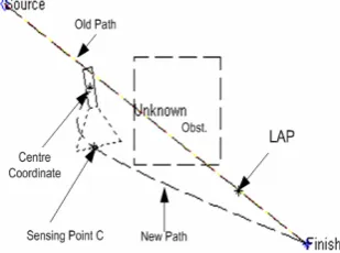
Fig. 9, illustrates the robot turning right according to step 2 as it encounters a random obstacle with the left side of the sensors and a new spline being generated as described above.
Fig. 9. Random Obstacle Avoidance
Step 4 The originally calculated optimal (i.e. before collision avoidance) path (fig. 9) is composed of many line segments. To find a suitable LAP we first have to find the point on a line segment on the optimal path which is closest to the robot’s current position. This will enable the robot to return onto the optimal path, once the obstacle is cleared. The following possibilities exist:
Possibility 1: In fig. 10, P indicates the coordinates of the current position of the robot and the line segment, P0 and P1 is the segment in consideration. The
following can be derived:
0 b
w=P −P = −ve (10)
ve P P
v= 1− 0 =+ (11)
ve
wv
C
1=
=
−
(12)Thus, if C1 is smaller than (or equal to) zero the robot
is on the left hand-side of the line segment P0 and P1.
Fig. 10. Robot on the left hand side of the segment
Possibility 2: The following are derived from fig. 11
ve P
P
w= b − 0 = + (13)
ve P
P
v = 1 − 0 = + (14)
ve
vv
C
2=
=
+
(15)ve
wv
C
1=
=
+
(16)Now if w≥ v then C1 ≥ C2 and the robot will be
[image:4.595.317.509.299.379.2]on the right hand-side of the line segment P0 and P1
Fig. 11. Robot on the right hand side of the segment
Possibility 3: If neither 1 nor 2 above are valid, then it must be the case that the following are valid:
ve P
P
w = b − 0 = + (17)
ve P
P
v = 1 − 0 = + (18)
v w vv wv C
C
b = = =
2
1 (19)
bv P
[image:4.595.317.511.416.598.2]Pb = 0 + (20)
Fig. 12. Robot above the segment
As it has already been mentioned, the original path is composed of many short line segments and we can find the point on the line segment that is closest to the current position of the robot by checking the distance between the coordinates of the robot and all the line segments on the original path using the aforementioned approach.
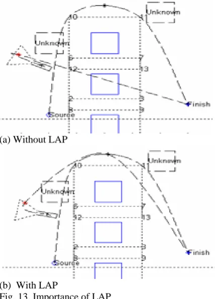
[image:4.595.63.218.446.561.2]round the known obstacles (solid lines). When an unknown obstacle (dotted lines) appear in the path a new path is calculated. Without a LAP the path may be too “sharp” for the robot to follow or one leading the robot into problems, fig. 13(a). With a LAP the path is smoother and easy to follow, fig. 13(b).
(a) Without LAP
[image:5.595.313.532.73.463.2](b) With LAP
Fig. 13. Importance of LAP
If the distance between the robot and the goal is shorter than that between the robot and the LAP then the LAP is ignored. If it is not ignored the robot will deviate from its path unnecessarily and may take a long time to recover.
Step 6 In the example shown (fig. 9), the sensing point C (fig. 6) is used as one of the control points for evaluating the new path. If the steering angle is negative (moving right), then the sensing point used as a control point for the R.O.A algorithm will be the sensing point C and if the current steering angle is positive then the sensing point B is used instead. The reason for choosing sensing points B or C rather than the robot middle point, is that the latter is more likely to result in a new path likely to lead the robot into collision with the obstacle. By choosing the sensing point C, the new path is further away from the obstacle. Similarly, if points A or D were chosen then the likelihood of a wider path (therefore likely to collide with other objects) increases.
Figures 14 and 15 show the importance of the LAP. In fig. 14(a) and 14(b), although the robot eventually reaches the goal, it orbits around the obstacle before it does so. This is due to the wrong values of LAP which can cause the robot to keep going round the object unnecessarily before it finally finds its way towards the goal. In contrast, the robot reaches the
goal optimally in fig. 15(a) and 15(b) resulting from a correct value of LAP.
(a)
(b)
Fig. 14. Using incorrect LAP values
(a)
(b)
Fig. 15. Using correct LAP values
Step 7 By using the centre coordinates of the robot, the sensing point, LAP and the goal as control points we can now create a new path using the Cardinal Spline. If more obstacles are detected on the defined path, repeat the previous steps until the robot reaches the goal.
4. IMPLEMENTATION OF THE ALGORITHM
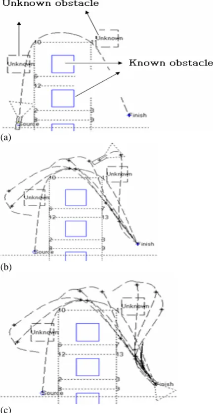
In fig. 16, dotted and solid lines indicate unknown and known obstacles respectively. The optimal path shown in fig. 16(a) is generated by consideration the presence of known obstacles only using a modified version of Dijkstra’s algorithm not discussed here.
[image:5.595.63.277.129.427.2]follow the predefined optimal path towards the goal. When unknown obstacles are met however, the procedure described in this paper takes control to modify the path and move the robot safely towards the goal whilst staying as close to the optimal path as it is physically possible.
(a)
(b)
[image:6.595.62.278.127.544.2](c)
Fig. 16. Simulation Results
5. CONCLUSIONS
In all simulation examples we have tried the R.O.A algorithm results in a fast and fairly smooth motion and within the competence of its sensing system will always find an optimal path and track it as much as it is possible. In producing these results, we have assumed that a) the robot cannot reverse and b) there is no disturbances and noise in the sensing system.
In generating the algorithm we have made use of a Look Ahead Point (LAP). It should be noted that the latter is dependent on the size of the obstacle encountered which, of course, for random or unknown obstacles will generally be unknown. Our solution relies on an educated guess based on information about the position of the robot, the coordinates of the point on the line segment
considered closest to the robot and the known goal or optimal path position. Choosing the wrong LAP value consistently results in the situation shown in fig. 14. Note that in this case the algorithm will not fail but it will lose efficiency. One possible solution is not to use a LAP until some mapping of the environment has been made. Although a jerkier motion may be generated, the algorithm still works. Choosing the correct values of safety margins and steering angle is also essential. Large safety margins provide the robot with more safety but it is possible that a path may not be found when one exists. It is best if moderate values are used which can then be increased or decreased based on acquired knowledge. In our case the safety margins used were directly related to the speed of the robot.
Increasing the magnitude of the steering angle also provides the robot with a sharper, thus quicker, turn when avoiding obstacles. However, the value has to be within reasonable bounds which depend on the physical limitations of the robot.
Improving the sensing system requires more computing power and therefore the capacity and memory of the robot has to be taken into account, as the algorithm is meant to work in real-time.
Finally, we have not presented any results regarding the convergence of this simple algorithm since the approach is heavily dependent on sensory inputs and the Look Ahead Point. The selection of the latter is empirical and thus a theoretical evaluation of convergence becomes almost meaningless in this case. However, an in-depth analysis is in preparation for a journal publication.
REFERENCES
Hausner, A. (2001) Parametric Curves,
http://www.dgp.toronto.edu/~ah/csc418/fall_2001 /notes/curves.html
IBM Corporation, GL3.2 Version 4.1 for AIX: Programming Concepts (POWER-based Systems Only),
http://publibn.boulder.ibm.com/doc_link/en_US/a _doc_lib/aixprggd/gl32prgd/gl32prgd02.htm#ToC Munoz, V. F. and Ollero (2003), A. Smooth trajectory
lanning method for mobile robots, Spain, ttp://webpersonal.uma.es/~VFMM/PDF/p05.pdf
p
h
a m
D h
Ringdahl, O. (2003). Path tracking and obstacle voidance algorithms for autonomous forest
achines, MSc Thesis in Umea University, epartment of Computing Science, ttp://www.cs.umu.se/~ringdahl/exjobb/
Twigg, C. (2003), Catmull-Rom splines,
http://graphics.cs.cmu.edu/nsp/course/15-462/Fall04/assts/catmullRom.pdf