The measurement of gains and losses from agricultural research

by

RAHMATOLLAH FARD SARHANGI, B.Sc. (Ag)

A dissertation submitted in partial fulfilment of the requirement for the degree of

Master of Agricultural Development Economics in the

AUSTRALIAN NATIONAL UNIVERSITY

D E C L A R A T I O N

Except where otherwise indicated, this dissertation is my own work.

R. Fard Sarhangi

This study was carried out while I was a student at the Australian National University, Canberra, on a Colombo Plan Scholarship offered by the Government of Australia. I am grateful to the Government of Australia for its generosity. Also, I extend my special gratitude to the Government of Iran and Mr Moeini Zand for granting me the necessary leave to undertake this study.

I must acknowledge the invaluable supervision that I received from Dr Ron C. Duncan, of the Industries Assistance Commission, Canberra. Despite the heavy pressures of work, he not only made himself available whenever I needed his help and guidance but also carefully read through all the drafts and made a great number of useful comments and suggestions. I owe him a profound debt of gratitude.

I must acknowledge my sincere gratitude to Dr Dan Etherington, the Convenor of the Master's Degree Course in Agricultural Development Economics, Research School of Pacific Studies, The Australian National University. By his advice and guidance he gave me great encouragement for this study.

To Dr Mark Saad, Fellow in the M.A.D.E. Program, of The Australian National University, I owe more than can be expressed here. His valuable encouragement in my work is greatly appreciated.

My thanks also go to Mr John Logan, Lecturer in Economics in the School of General Studies, The Australian National University, for his help and suggestions regarding some mathematical problems in

Chapter 4 of this study.

I also would like to thank those people who did the typing of the initial draft.

Lastly, deepest debt of gratitude goes to my wife Nasrin, who was a continual source of love and inspiration.

Canberra

C O N T E N T S

Page

Acknowledgements (ii)

Abstract (v)

List of Tables (vi)

List of Figures (vii)

CHAPTER

1 INTRODUCTION 1

2 MEASUREMENT OF TOTAL SOCIAL GAINS FROM RESEARCH 5

2.1 Introduction 5

2.2 Supply-Shift Method 6

2.2.1 Griliches' Method 6

2.2.2 Peterson's Method 19

2.2.3 Comparison of an Alternative Formula 23

2.3 Input-Demand Method 35

2.4 The Appropriateness of Using Supply Analysis

Versus Input-Demand Analysis 43

3 DISTRIBUTION OF RELATIVE GAINS (LOSSES) FROM

RESEARCH AMONG PRODUCERS AND CONSUMERS 51

3.1 Introduction 51

3.2 Akino and Haxami's Method 52

3.3 Ayer and Schuh's Method 58

3.4 Studies by the Industries' Assistance

Commission 66

3.5 Comparison of Ayes and Schuh and I.A.C. Methodology for Analysis of Distribution

of Net Social Gains to Research ^2

4 SPECIFICATION PROBLEMS 82

4.5 Comparisons with Scobie's Results

5 DISTRIBUTION OF THE GAINS (LOSSES) FROM RESEARCH AMONG FACTORS OF PRODUCTION

5.1 Introduction

5.2 Schmitz and Seckler's Method 5.3 Minimum Wage Implications 5.4 Re-Qnployment Possibilities

5.5 Compensation for Displaced Labour

6 CONCLUSION

91

94 94 94 102 107 109

116

A B S T R A C T

This thesis is a survey of research over the last two decades stemming from the now classical study by Griliches on

evaluating the gains from agricultural research. The thesis points to a number of areas in which there are problems which need to be resolved, and hopefully, in a few instances provides the basis on which future research may proceed.

The most important point of concern is the under-estimate of social gains (losses) provided by the supply-shift approach

developed by Griliches. Wisecarver has shown that estimates based on shifts in input-demand curves are an appropriate method of estimating such gains.

The several studies which have attempted to estimate the distribution of productivity gains between consumers and producers were shown by Scobie to have used formulations of consumers' and

LIST OF TABLES

Table Title Page

2.1 Demand Elasticity/Reduction of Costs Matrix 14

3.1 Estimates of Average Annual Benefit in Japan

from Rice Breeding Research (Million Yen

in 1934-36 Constant Prices) 57

3.2 Estimated Internal Rates of Return (Per Cent)

Under Various Assumptions Concerning Elasticity of Supply and Demand and the

Shift Factor K 65

3.3 Distribution of the Direct Benefits of Rural

Research 73

3.4 Maximum Effect of Two-Price Schemes on

Distribution of Direct Benefits of Rural

LIST OF FIGURES

Figure Title Page

2.1 Downward Shift in the Supply Curve Due to

Adoption of Cost-Reducing Innovation 7 2.2 Upward Shift in the Perfectly Elastic Supply

Curve Due to the "Disappearance" of Hybrid Corn 8 2.3 Leftward Shift in the Perfectly Inelastic Supply

Curve Due to the "Disappearance" of Hybrid Corn 10

2.4 Proportionate Shift of Supply 11

2.5 Changes in Industry Surplus with Perfectly

Inelastic Demand 15

2.6 Producers' and Consumers' Surplus Changes from

Supply Shift 17

2.7 Shift in the Supply Schedule Resulting from

the Use of New Inputs 20

2.8 Parallel and Non-Parallel Shift in Supply with

Unitary Arc Elastic Demand 25

2.9 Diagrammatical Representation of Equation to Measure "Ex-Ante" Gains from Research Which

will Result in a Shift of the Supply Curve 27 2.10 The Gains from an Increase in the Productivity

of an Input 36

2.11 Effects of a Tax Distortion in Input and Output

Markets 46

3.1 Model of Estimating Social Returns to Rice

Breeding Research 53

3.2 Social Returns Due to Supply Shift 60

3.3 Rightward Shift of the Supply Curve Due to an

Increase in Productivity 67

3.4 Social Gains Resulting from an Increase in

Figure Title

4.1 Social Return from a Parallel Supply Shift 5.1 Effect of the Tomato Harvester on Employment

of Farm Workers

5.2 Effects of the Tomato Harvester on Employment of Farm Workers with both Perfectly Elastic Supply and Inelastic Supply

Page

90

101

CHAPTER 1 INTRODUCTION

"Technological change" by definition consists of two major types:

(a) reduction of real costs per unit of output

(increasing productivity in resource use); and

(b) improvements in the quality and variety of final consumption goods.

John W. Kendrick (1964) considered the "gains and losses" from technological change on two different levels. Firstly, the absolute gains and losses which accrue, on net balance, in the economy as a whole and its sectors. Secondly, relative gains and losses that accrue as a result of changes in relative prices of the various factors of production and intermediate inputs. The first type of gain or loss may be easily quantified, but relative gains and losses are much more difficult to

quantify, since relative input prices change for reasons other than techno­ logical change and we have to attempt to separate out the relative price changes among the several causative factors.

Technological advance is reflected in net changes in total factor-productivity. Annual gains can be estimated by applying the average productivity of the previous year to the factors which are

it would be better to compute productivity increments over longer periods of time which can be done by the same technique". In a similar fashion the total productivity increase can be assigned to all the original industries. So much work has been done on the abso­ lute level of productivity gains, but what about the distribution of the benefits and losses which are realised in the process; especially the earnings lost by those unemployed people whose dis­ placement may be traced to technological change?

Part of the costs of persons thrown out of employment on account of technological progress is borne by the community in the form of unemployment benefits. The employer may bear part of the cost in terms of redundancy payments, and the employee bears part of the costs in terms of income foregone. To what extent and in what manner should these costs be taken into account when assessing the impact of technological change?

As well as having the effect of increasing or decreasing the earnings potential of some labour, technological change can also increase or decrease the income earning potential of existing capital and land.

All of the important problems involved in answering the various questions implicit in the above statements about distribution have been barely touched upon in research in this area. This thesis sets out to review the progress made so far in looking at the benefits and costs of research and the distribution of these. The thesis

points out a number of areas where further research is needed, and attempts to reconcile some of the differences which have arisen in the development of research techniques.

Organization of the Study

Measurement of total social gains from research is discussed in Chapter 2. Two issues are elaborated; one is sorting out the real supply shift due to a particular research program from other factors influencing supply. A second has to do with the type of supply shift. The Lindner-Jarrett discussion (1976) stresses the fact that research produced technology is not generally equally relevant to all producing

environments and that this fact can affect the measurement of the supply shift. Two techniques which have been used for measuring the gains from research are discussed - the supply-shift method and the input-demand method. In the light of the analysis by Wisecarver (1974) of the validity of the answers provided by the supply-shift method, the con­

the same circumstances. Chapter 5 deals with the allocation of

CHAPTER 2

MEASUREMENT OF TOTAL SOCIAL GAINS FROM RESEARCH

2.1 Introduction

In this chapter the development of the two different

techniques of analysing social gains (losses) generated from productivity-increasing research are reviewed. The two methods of estimation of

social gains (losses) presented in this chapter are:

(i) the Supply-Shift method; and (ii) the Input-Demand method.

The first method measures social gains in terms of the output response to lowering the costs of production. The Input-Demand method measures the social gains from research by estimating the increase

in the demand for that input whose productivity has been increased as a result of research.

2.2 Supply-Shift Method

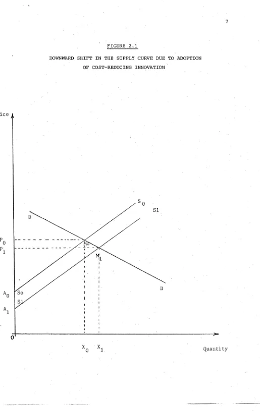
At the industry level, the effect of the adoption of a cost-reducing innovation can be represented diagrammatically by a downward shift of the supply curve. This means that more output can be produced at a given price, or the same output can be produced more cheaply. Economists now generally have agreed that the gross social benefits of the research which produces the innovation can be measured by the area between the two supply curves and below the demand curve.

In Fig. 1, S S represents industry supply curve in the absence of o o

the innovation, and is the supply curve when the innovation is adopted. The area to be measured is given by •

Although there is now general agreement about the area to be measured, the estimation methods used have varied greatly, and there has been a tendency to cover up the implications of the assumptions about the nature of the shift of the supply cruve.

2.2.1 Griliches1 Method

FIGURE 2.1

DOWNWARD SHIFT IN THE SUPPLY CURVE DUE TO ADOPTION OF COST-REDUCING INNOVATION

DUE TO THE "DISAPPEARANCE" OF HYBRID CORN

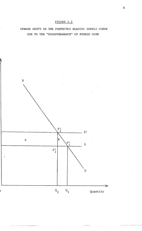
the "loss" to society, in this case is the total area under the demand curve and between the new and old supply curves, which is (A + B). Griliches considers the rectangle A as the increase in the total cost of producing the quantity in the new situation, and the triangle B as the loss in consumer's surplus caused by the rise in price. A linear approximation of the area (A + B) is given by the following formula:

Loss 1 = KP^Q^ (l-i^Kri) where,

K = % change in yield (marginal cost and average cost) = previous equilibrium price of corn produced

= previous equilibrium quantity of corn produced

T) = price elasticity of demand for corn

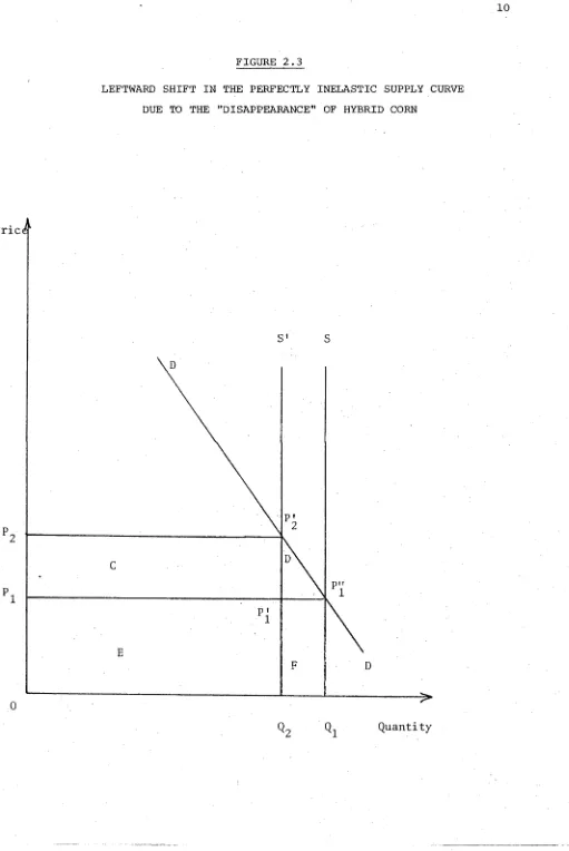
Secondly, he assumes that the elasticity of the supply curve is zero (Fig. 2.3). In this case, the loss should be measured by the area Ö2P2P1^1 ^or D + * T^e rectangel, F, measures the loss is corn production at P^ which is the old price. The triangle, D, is the deadweight loss in economic welfare. C + D is the loss in consumer surplus. The total loss is given by the formula:

Loss 2 = KP Q (1+^Kn).

FIGURE 2.3

LEFTWARD SHIFT IN THE PERFECTLY INELASTIC SUPPLY CURVE DUE TO THE "DISAPPEARANCE" OF HYBRID CORN

FIGURE 2.4

PROPORTIONATE SHIFT OF SUPPLY

P

Ao

p. 1

A 1

Ai

D Q = q

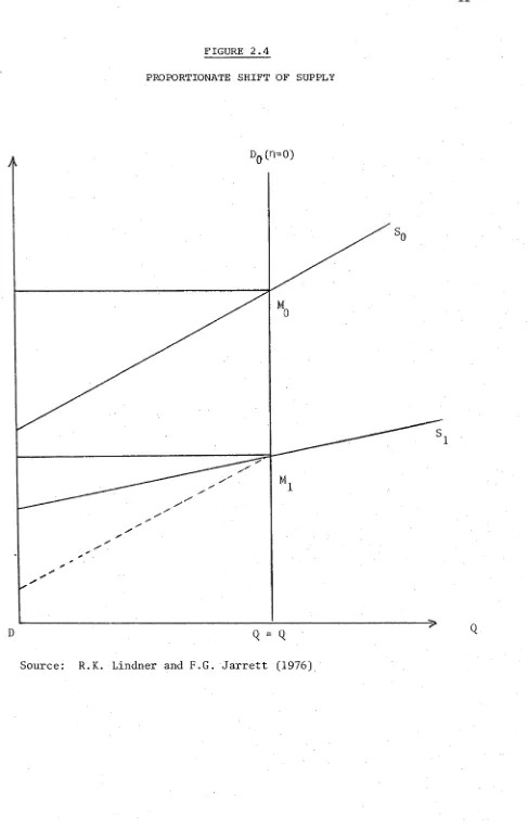
implies that the reduction in average cost of production is greater at the margin than at intra-marginal levels of output.

They point out that an innovation of hybrid corn type is likely to result in a proportionate shift rather than a parallel shift in the supply curve because it is almost certain that the long-run corn supply curve will be less than perfectly elastic, and positive change in yields of hybrid corn may be relatively constant in all areas. If this is the case, Griliches' estimates of actual benefits could have been biased upwards.

Lindner and Jarrett have also shown that for a parallel

shift of a partly elastic supply curve Griliches' formula under-estimates actual benefits when demand is not perfectly elastic, and that the error magnitude becomes larger as the demand curve elasticity increases. As a result, "Two biases operating in opposite directions will be intro­ duced by using Griliches' formula to estimate research benefits when both demand and supply are neither perfectly elastic, nor perfectly inelastic. It is therefore not possible a priori to reach a definite conclusion about whether Griliches has over-estimated the returns to hybrid corn research.".

be reduced to KP^Q^. This KP^Q^ actually measures the area P^M M^P^ in Fig. 2.4. Now, we should refer to W. Clayton Dodge (1972) for the Law of Parallelograms, which says "the area of any parallelogram is equal to that of a rectangle with the same base and altitude". Thus, taking this Theorem into account, the area P M M,P„ is equal to the

o o 1 1

area A M M..A *. According to Lindner and Jarrett, since the area o o 1 1

AqMqM^A^* would represent the level of research benefits for a parallel downward shift of the supply curve, the above formula will over-estimate these benefits (by the triangle A^M^A^* in Fig. 2.4) whenever the absolute fall in average costs of production is greater (at the margin) than the reduction of costs infra-marginally and as long as demand is perfectly inelastic.

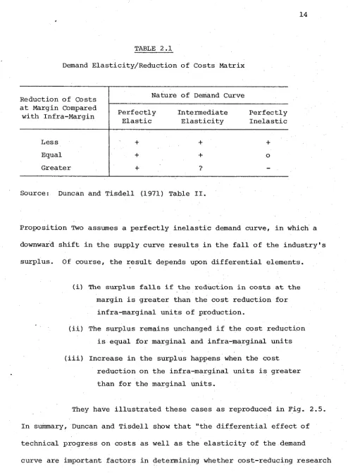
Duncan and Tisdell (1971) have shown that differences in the reduction of costs at the margin compared with infra-marginal

reductions for different demand elasticities are important in assessing the influence of cost-reducing technical progress on an industry's profit, or producer's surplus. As shown in Table 2.1, the columns of their

matrix represent the nature of the elasticity of demand and the rows show the differential effect of technical progress on marginal and infra­ marginal costs. The signs +, - and o denote the variation in the

industry's surplus. In the bottom row, the question mark denotes that the outcome will only be clear if exact specification of the demand curve and the shift in costs are available.

Duncan and Tisdell present three "propositions" which corres­ pond to the columns. For simplicity, let us examine only the second

TABLE 2.1

Demand Elasticity/Reduction of Costs Matrix

Reduction of Costs at Margin Compared with Infra-Margin

Nature of Demand Curve Perfectly

Elastic

Intermediate Elasticity

Perfectly Inelastic

Less + + +

Equal + + o

Greater + •?

-Source: Duncan and Tisdell (1971) Table II.

Proposition Two assumes a perfectly inelastic demand curve, in which a downward shift in the supply curve results in the fall of the industry's surplus. Of course, the result depends upon differential elements.

(i) The surplus falls if the reduction in costs at the margin is greater than the cost reduction for

infra-marginal units of production.

(ii) The surplus remains unchanged if the cost reduction is equal for marginal and infra-marginal units (iii) Increase in the surplus happens when the cost

reduction on the infra-marginal units is greater than for the marginal units.

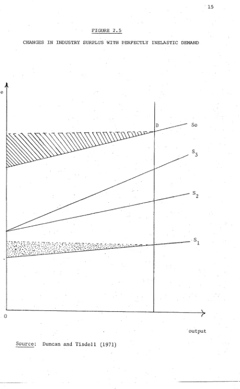
They have illustrated these cases as reproduced in Fig. 2.5. In summary, Duncan and Tisdell show that "the differential effect of technical progress on costs as well as the elasticity of the demand

FIGURE 2.5

CHANGES IN INDUSTRY SURPLUS WITH PERFECTLY INELASTIC DEMAND

price

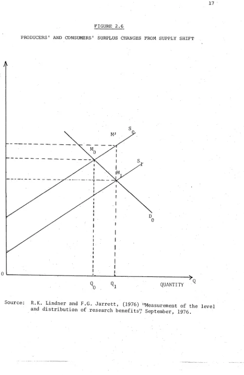
Lindner and Jarrett have depicted in Fig. 2.6 a different case, i.e., whe n demand and supply are neither perfectly inelastic

nor perfectly elastic. In this Figure, is parallel to Sq , and the

vertical distance between S and S, is measured by K P , , in which K

o 1 1

should be interpreted as the proportionate reduction in costs at o u t ­

put level only. Griliches' formula in this case is KP^Q^ (l-^Kg)

w h i c h under-estimates the correct area A M M,A, as follows:

1. KP1Q1 (1-^Kri) = KP1Q1 - feKTl) KP1Q1

the term KP, Q, measures P'M'M, P,

1 1 1 1

2. P'M'M, P, = A M'M,A, (by the law of parallelograms)

1 1 o i l

since g = the absolute value of the price-elasticity of demand for corn.

3. Then g AQ fi

AP Qx

Qr Q0

Po “ Pl

4. Substituting for g at P^, in the second term,

5.

KPpQi (^Kp) gives

KP1Q1 (^Kg) = KP1Q1 h k

0 - 0 P

yl yo # _L P " P -i ' Q n

O 1 1

KPi ei % k

cr Qo 1

P -P

o 1

%KPi [Ql-Qo ]

KP. P -P.

o 1

since the area of the triangle M'MoM, = %KP, (Q ,-Q ) and,

FIGURE 2.6

PRODUCERS' AND CONSUMERS' SURPLUS CHANGES FROM SUPPLY SHIFT

P R I C E

QUANTITY

6. KP P'-P,

1 1

Therefore,

(P'-P ) + (P -P,)

o o 1

7. KP., Q, (%KT1) = area of triangle M'M M n

1 1 o 1 1 +

P'-P P -P_

o 1 finally, the area which is to be measured correctly is equal to A M M. A, or

o o 1 1

8. A M M A

o o 1 1 A M'M A - M'M Mno i l o 1

This area is greater than the one measured by KP^Q^ (l-^Kq), by

the amount area of

fr

H*

T) 1 _TJ

0 _{____}

1

M'M M P ~Pn

o 1 O 1

I extent the equation 8, so:

9. A M'M A - M'M M, > KP O, (1-^KT|) o 1 1 o 1 1 1

or > KP Q - KP Q (^Kq)

or > Q [(P'-P ) + (Pq-P1 )] - KP Q (^Kq)

or > Q, [(P'-P ) + (P -P-, ) ] - M'M M

1 o o 1 o 1

1 + P'-P P -P_

o 1

The term M'M M, will be cancelled out on both sides, thereby o 1

I can write:

P'-P 10. A M'M A > Qn [(P'-P ) + (P -P ) ] - M'M M n

[---o 1 1 1 o o l o l P -Pn

o 1

11. A M'M ,A, > O P '

o 1 1 1 Q,p 1 o + Qip1 o 21P1 M'M Mo 1

P'-P or > Q, P' - Q,P, - M'M M, [--- — ]

V1 V1 1 o 1 P -P_ o 1

since A M'M., A should be equal to Q, P'-Q.P, (to hold the inequality)

and Q^P'-Q^P^ is equal to the area of rectangles 0 Q^M'P' and 0 Q^M^Pi respectively in Fig. 2.6, thereby:

A M'M A = O Q M ' P ' - O Q M P , = P'M'P M

o i l *1 1 1 1 1 1

P'-P

so, [the area of M'M^M^] [p - _ y ] is virtually the difference o 1

between the area measured by KP, Q, (l-^Kri) and the area A M M A .

1 1 o o 1 1 •

From the above, Lindner and Jarrett concluded that this under-estimation of research benefits by the formula (when demand is relatively elastic) generally will be balanced by the nature of the

formula to over-estimate benefits when reductions in cost for infra­ marginal production are less than those at the margin, "and the net bias introduced by using this formula is indeterminate". They developed an alternative general formula by which research benefits can be measured carefully and exactly which will be discussed later.

2.2.2 Peterson's Method

FIGURE 2.7

SHIFT IN THE SUPPLY SCHEDULE RESULTING FROM THE USE OF NEW INPUTS

PRICE

QUANTITY

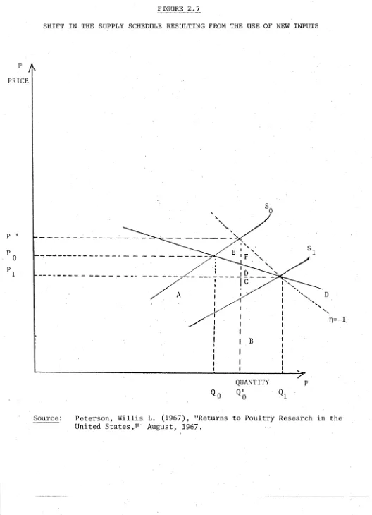
The first error is about the area between the two supply curves and below the demand curve. He refers to it as consumer surplus, whereas it is in general the sum of producer surplus and consumer

surplus. However, when supply is perfectly elastic, or when demand is perfectly inelastic AND there is a parallel shift in the supply curve, then increased social benefit will consist completely of consumer surplus.

The second error relates to the treatment of the variable K, defined as the percentage decrease in the supply function of poultry products that occurs if the new inputs used by poultry farmers to obtain higher efficiency disappear. However, in his actual treatment of K it is represented as the change in the equilibrium quantity of output if the innovation disappears; and, it is expressed as a proportion of the equilibrium level of output produced with the innovation, for example,

öö

K = — --- in Fig. 2.7. Peterson, in fact, is contradicting himself

by this definition of K which implies a horizontal, rather than a vertical shift of the supply curve. In addition, it understates the extent of the shift since it includes the effect of the equilibrating process which involves supply and demand together. "This approach

makes it more difficult to interpret the effect of agricultural research per se on the supply function, and would require the further education of scientists into the mysteries of supply and demand elasticities."

(Lindner and Jarrett, 1976).

they present a more precise diagram (Fig. 2.6), which shows the special case of a parallel shift in the supply curve and a demand curve which is unitary and elastic. By using this figure, they show that Peterson's assertion about the equality of the above two areas is wrong and they cannot, in general, be even approximately equal.

The areas A + C + D + E + F and B + C + D + F (from Peterson's diagram in Fig. 2.7) correspond to areas A M M,A, and

o o 1 1

Q^M^M^Q^ (in Fig. 2.6) respectively. When demand is unitary they are elastic: Q M M„ Q„ = P M M P . By the Law of Parallelograms, area

o o 1 1 o o 1 .

A M'M A. = area P'M'M, P, . So area A M M a. = area P'M'M, P, - area

o i l 1 1 o o l l 1 1

M M'M or A M A A > P M M , P, , by the area P'M'M P .

o 1 o o l l o o l l o o

Greg Martin et a l . (1977) believe that Peterson's formula is backward looking - completely expost, which requires the maximum possible amount of information and almost impossible to apply "ex ante".

Peterson's formula for calculation of the absolute size of the benefits is as follows:

B K Q1P1 + h KV l - ^2 , Q K2

n *o

(px ) (en) ( n - D pi p _o (n+e) (n)

where,

K is defined as the percentage shift to the left of the supply function, if the innovation had not been available to farmers. £ and n are the supply and demand elasticities.

Pl^l are e(lu ilit,rium price and quantity of poultry products after innovation.

Martin et a l . believe that the above formula is incorrect. However, they present a simpler and more elegant ex ante formula:

B KP Q

o o [1 +

k (i-k) n

2en

KG

]

where K is defined (vertically) as the proportionate reduction in unit costs as a result of the innovation. Also K is relatively simpler to obtain empirically.

2.2.3 Comparison of an Alternative Formula

As was pointed out earlier, both Griliches (1958) and Peterson (1967) assumed that an agricultural innovation would shift the supply function by the same percentage amount at all levels of output, and went forward to measure the benefits from the innovation by raising the question: "What would have been the losses if this innova­ tion were to disappear?". However, (instead of this indirect approach) Lindner and Jarrett (1976) suggest that it will be more helpful in evaluating the impact of research on agricultural production if we take the direct approach of measuring the gains from research relative to the pre-innovation market equilibrium. A research manager, in making decisions about the amount of resources required or desired to be allocated to agricultural research, knows the situation of the current supply and has to make estimates of the impact of the research on future supply conditions. That is to say, he needs to estimate

For simplicity, Lindner and Jarrett assume, as an approxi­ mation, linear supply and demand functions. Now, with reference to Fig. 2.8, S and D denote the initial supply and demand functions

o o

prior to innovation. According to them, if we postulate a proportionate shift in Sq , which implies that the reduction in average costs is

greater at the margin than at infra-marginal levels of output, then will reflect the new, post-innovation, supply function. They suggest

that "treating the movement of the supply function as a vertical, rather than a horizontal, shift emphasizes the cost-reducing nature of innova­ tions, and is the way in which research scientists can more easily understand the effect of their research on the supply of agricultural output".

In Fig. 2.8, the area A., M, M A which represents the gain in 1 1 o o

consequent to the innovation, can generally be measured by the rule of cross-multiplication. This rule is developed by J.F. Durrant and H.R. Kingston (1946) and relies on the co-ordinates of the points A ^ , M, , M , A which are expressed in an anti-clockwise direction. The

l o o

co-ordinates are: 0, A, , Q, , P, , Q , P and 0, A respectively. Now

1 X1 1 *o o o

the area of this rectilinear figure (A„ M, M A ) which can be separated 1 1 o o

into the areas of a series of triangles may be obtained by:

[0 x Pn + P x Q, + Q x A + 0 x A n - 0 x A - O x P - P, x Q

1 o *1 *o o 1 o o 1 *o

-

Q

which is equal to

h [P Q - P-.Q + Q A - Q A ]

FIGURE 2.8

PARALLEL AND NON-PARALLEL SHIFT IN SUPPLY WITH UNITARY ARC ELASTIC DEMAND

P

A

QUANTITY

The above two expressions presented by Lindner and Jarrett can be derived as follows.

First, I consider the quadrilateral Z^ Z^ (Fig. 2.9) where, by construction, we have:

BCDE as a rectangle

B Z_ G 7, A as another rectangle 3 4

Therefore,

A

A

3 4 3 4

Similarly,

A c z2z3 -

A

A D Z ^

A

A

z„ =

1 4

A Z l K Z

4

Adding both sides of all equations and using Fig. 2.9 we have

BCDE - Z1 Z2Z3Z4 = Z Z Z Z + IHGK

or ZZ.Z^Z.Z, = BCDE - IHGK 1 2 3 4

since area BCDE = (Y3 - Y^) (X2 - X4 )

= BE x DE and area IHGK =

_{(Y2 - V}

(X3 -

V

Therefore,

2Z1Z2Z3Z4 = BCDE - IHGK

FIGURE 2.9

Y X„ + Y, X - Y X Y X -3 2 1 4 1 2 3 4 [Y„X_ + Y . X.. - Y . X_

_{- Vi1}

2 3 4 1 4 3

Y X„ + Y n X, + Y . X_ + Y_X._ 3 2 1 4 4 3 2 1 Y X„ Y_X_ - Y X

3 4 2 3 4 1

Therefore,

Z Z Z Z *2 Y X + Y X + Y.X_ + Y„X--3 2 1 4 4 3 2 1

Y2X3 - Y4X1 - Y3X4 - Y1X2 (3)

In Fig. 2.8, we have the rectilinear A. M_M A , but for simplicity, 1 1 o o

M = (Q , P )

o o o

1 - (

V V

let us call it Z^Z^Z^Z^,

Then,

X = 0 and -> Z = (X , Y1 )

Similarly,

3

oP

II _and

Y3 = Po ^ z3 (X3 ,

V

4 =

0

o1

*

<V V

If we substitute the above in (3), we will have the same expression as in (2). Hence,

Z Z Z Z = % p

o X Q , + A1 x 0 + A x o Q + P x 0 o 1

pi X 2o - Ao x 0 - P o X 0 - Ax x Q1

= k (P x Q + A x Q - P x Q - A x Q ... (2')

o 1 o o 1 o 1 1

From (3) , we can write (in a vector form)

Z Z Z Z = h [X X X X ]

Equation (4) is equal to (3).

Now, if we substitute for X^, in equation (4) we will have

Z Z Z Z ^ [0 Qx Qo 0]

P, - A P - A, A - P. A, - P

%[Si(p0 - V + 2o <Ao - V 1 (2")

As was mentioned earlier, Griliches' measure of research benefit assumes a perfectly elastic supply curve. Lindner and Jarrett

The expression for the surplus in this special case is

%[P Q, - P-, Q + P 0, - P,Q, ] . The expression used by Griliches is o 1 1 o o 1 1 1

Loss 1 = KP^Q^ [1 - % K p ] . K is the proportionate shift in the supply

Po - P-l

function measured in a vertical direction and K = --- in Fiq. 2.4 pi

If we evaluate the absolute value of the elasticity of demand p (at P , ) / then:

If we substitute for K and p in the expression for Loss 1 then:

P - P P

_o___ ^1_ A Q b ll_ P-L AP ' Q1

and this reduces to: Loss 1

P -

o

P 0 1V1

Loss 1 k[P Q - P Q

2L

oyl

1*0

V i 1

From above, Lindner and Jarrett claim that equation (5) is the same as the result derived from the general expression in equation (2). Also, in the more general case when supply is less than perfectly elastic,

the formulae in equations (2) and (3) are obviously not equal. The

important point in equation (3) is that it measures the level of consumer benefits arising from adoption of the innovations, whereas, equation (2) measures total social producer benefit plus consumer benefit.

T h e r e f o r e ,

(6)

Within the assumptions made, equations (2), (5) and (6) are

Lindner and Jarrett's general results. Their applications require a

knowledge of the original equilibrium price and quantity P , Q^; the

new equilibrium price and quantity P_ , Q ; and values for A and A.,.

1 1 o 1

They point out that where research results have already been incorporated into production processes and an "ex post" measure of research benefits

is to be calculated, data on P^ and , i.e., current equilibrium price

and quantity, can be obtained. Nevertheless, the variables P , Q , A

o o o

and A^ have to be estimated indirectly. We may get extra difficulties

in applying the formulae "ex ante", as variables cannot be observed

directly. The reason is that P , Q are sensitive to other unknown

o o

influences in addition to the adoption or non-adoption of the innovation. However, given a relatively stable condition of demand and supply, we

can obtain reasonable estimates of P and Q from current levels of

o o

industry price and output. In order to estimate P^ and , the following

formulae can be used:

(7)

(8)

In the above two formulae (adapted by Lindner and Jarrett

reduction in average costs of production, measured at , from adopting the new technology; £ and rj are the price elasticity of supply and demand respectively. We can make cost-reduction estimates by using the methods pioneered by Griliches (1958) and Petersen (1967) for "ex post" calculations, but "guess-timates" would have to be made in any

"ex ante" evaluation of research proposals. The values of and in the nearness of P , Q and P, , Q_ can be estimated by widely-known

o o 1 1

econometric techniques.

The problems associated with estimation of in the case of "ex post" studies, or A for "ex ante" studies, are not so easy to

o

control. In general, Lindner and Jarrett do not believe that econo-metrically estimated supply curves will provide reliable estimates of An (or A ) because the available observations on P and Q used to

calcu-1 o

late supply parameters are typically far removed from the point where the supply curve intercepts the vertical axis. Actual estimates of supply curves often involve negative intercept terms. Such an abnormal case need not matter if the estimated supply curve is only to be used to project prices and/or quantities in the nearness of the original data set, but in their case, it is obviously illogical as it implies that producers are prepared to supply positive quantities at zero price in the long-run. Instead, they believe that A^ (or A^) can best be estimated by asking industry experts the following question:

f a c t t h a t t h e e s t i m a t e d l e v e l o f r e s e a r c h b e n e f i t i s r e l a t i v e l y

i n s e n s i t i v e t o t h e v a l u e o f A, ( o r A ) u s e d i n t h e f o r m u l a .

1 o

E s t i m a t e d b e n e f i t s o f r e s e a r c h a r e , n e v e r t h e l e s s , m uch

m o re s e n s i t i v e t o t h e n a t u r e o f t h e s h i f t i n t h e s u p p l y c u r v e i n d u c e d

b y a d o p t i o n o f t h e i n n o v a t i o n w h i c h , g i v e n A . , d e t e r m i n e s A , o r t h e

1 o

o t h e r way r o u n d . G r i l i c h e s ' a r g u m e n t s (1 9 5 8 ) f o r a p r o p o r t i o n a t e

s h i f t i n t h e c a s e o f h y b r i d c o r n , seem c o n v i n c i n g , b u t t h e y a r e o n l y

a p p l i c a b l e t o l o w - c o s t i n n o v a t i o n s w h i c h i n c r e a s e y i e l d s b y a n e q u a l

p r o p o r t i o n a t e a m o u n t f o r a l l p r o d u c e r s .

The a b o v e d i s c u s s i o n i n d i c a t e s t h a t t h e t o t a l l e v e l o f

a n n u a l s o c i a l b e n e f i t s f r o m a d o p t i o n o f a n i n n o v a t i o n i s a f f e c t e d b y

t h e n a t u r e o f t h e s h i f t o f t h e s u p p l y c u r v e . C o n s e q u e n t l y , t o e s t i m a t e

a g g r e g a t e b e n e f i t s f r o m r e s e a r c h , i t i s n e c e s s a r y t o e s t i m a t e t h e e f f e c t

o f a d o p t i o n o f t h e i n n o v a t i o n o n t h e a v e r a g e c o s t o f i n f r a - m a r g i n a l

p r o d u c t i o n t o g e t h e r w i t h i t s e f f e c t o n e q u i l i b r i u m p r i c e a n d q u a n t i t y

o f i n d u s t r y o u t p u t . The m o s t c o n s p i c u o u s p a r t o f t h i s d i s c u s s i o n i s

t h e n e e d t o g i v e e x p l i c i t r e c o g n i t i o n t o t h e r e l a t i o n s h i p b e t w e e n A o

a n d A ^ , t h a t i s , t o t h e n a t u r e o f t h e s h i f t i n s u p p l y f u n c t i o n . I f

we c o n t r a s t L i n d n e r a n d J a r r e t t ' s r e s u l t s w i t h t h e a t t e m p t s o f G r i l i c h e s

( 1 9 5 8 ) , P e t e r s o n (1 9 6 7 ) a n d A k i n o a n d H a y am i (1 9 7 5 ) i n t h e i r s t u d i e s

a t m e a s u r i n g r e s e a r c h b e n e f i t s , we w i l l n o t i c e t h a t e a c h o f t h e s e

s t u d i e s h a s v i r t u a l l y m ade i m p l i c i t a s s u m p t i o n s a b o u t A^ a n d A ^ . F o r

e x a m p l e , G r i l i c h e s , b y a s s u m i n g p e r f e c t l y e l a s t i c s u p p l y c u r v e , u s e s

P a n d Pn a s t h e e s t i m a t e o f A a n d A, r e s p e c t i v e l y ; w h e r e a s A k i n o

o 1 o 1

a n d Hayami a s s u m e t h a t A^ a n d A^ a r e b o t h c o i n c i d e n t w i t h t h e o r i g i n .

S u c h a s s u m p t i o n s do n o t se e m v e r y p l a u s i b l e . M o r e o v e r , L i n d n e r a n d

are subsumed in the estimating procedures used to calculate the supply elasticity, and where A^ is pre-calculated by Aq and the assumption of a proportional shift in the supply function, as equally "unsatisfactory". Particularly, when we do not see any good reason (in general) why the shift in the supply curve should be proportional rather than parallel, pivotal about A ^ , or convergent.

In conclusion, as it seems unreasonable from empirical evidence to support Griliches1 assumption of a perfectly elastic supply curve, then it follows that his formula will over-estimate the measure of research benefits. Similarly, even though Peterson's formula takes

into account the effects of supply and demand elasticities, over­ estimation of benefits will still result.

The usefulness of the methods to the problem of allocation of resources in research is important. Both Griliches and Peterson's

approaches are restricted to evaluation of research results after the research has been done and made available to producers. However, equation (2) from Lindner and Jarrett allows prediction of benefits prior to undertaking the research and thus decisions can be made on whether or not to undertake the research.

2.3 Input-Demand Method

R.C. Duncan (1972) attempted to identify pasture research findings which have been important for the development of improved pastures in some agricultural regions in Australia and to estimate the

IRR on the investment in pasture research in those regions. His tech­ nique is based on the estimation of input-demand functions for the stock of improved pastures.

He estimated the contribution made by individual research findings rather than estimating the benefits flowing from research by the output supply-shift used by Griliches since this method would not have been suitable in those circumstances. This is so because the adoption of new pasture technology by farmers is not directly observ­ able in yield responses such as an increase in wool or beef. The

input-demand method becomes a means of estimating the benefits generated by an increase in the productivity of an input, which in this case has been improved pastures.

To illustrate, take Fig. 2.10 in which the input-demand curve is assumed to have a negative slope; ID^ and ID^ are input-demand curves prior to an increase in productivity and after an increase in productivity, respectively. The hatched area (given certain assumptions) represents the gross welfare gains from the increase in productivity. It is the value of this area which he estimates.

A

input price

A

j

0

to ID^/ which implies a non-parallel shift of the curve in its non­ linear form.

The movement from Q to usually involves a number of years taking account of the lagged adoption of the new technology.

In this time the price of product and the price of input could have been changed. For calculating purposes he strongly assumes that the shift from ID^ to ID^ relates to some ID curve based on an average product price for the period of the shift from to Q . Also, it has to be assumed that the input price is some average of the cost of improving pastures during the period.

A single-equation regression model is formulated which is used to estimate (i) input own-price elasticity of demand, and identi­ fies (ii) important research findings. From (ii) Duncan estimates

the shift from Q, to . From (ii) and (i), he derives (by integration)

1 2

a formula which gives an estimate of the gross value of the hatched area (see Fig. 2.10). In the model,

(a) the area of improved pastures on farms in

selected areas is treated as a durable input, and

(b) the demand for the stock of improved pasture is a function of its real price and the state of pasture technology,

Three dynamic aspects of the shift from ID^ to ID^ should be cited: firstly, the shift from to does not occur instantan­ eously. It appears, for that reason, that the long-run elasticity of input demand is the relevant one. Secondly, the improvement in

technology may be lost over time due, for example, to pests, insects and diseases. Thirdly, the input demand curve can also shift with changes in product prices, and this will change the size of the hatched area for a given improvement in technology. Therefore, estimation of the discounted value of future benefits involves predictions about the price of products.

Duncan's model is a dynamic interpretation of the neo­ classical theory of the demand for an input. According to the static theory of the competitive firm, every decision maker wishes to maximize his profits within a framework of input-output relationships and price ratios, instant adjustment and unlimited capital. Also, the individual's decisions for production under perfect competition have no effect on prices. Stigler (1952) points out that within such a static framework changes in demand for an input will depend on:

(i) changes in the product price;

(ii) changes in the input cost and in other inputs cost, and

(iii) changes in the productivity of the input.

Jorgenson (1963) shows that under certain assumptions the demand for the services of a durable input (such as improved pastures in this study) depends on its real price and relative price. We cannot usually measure the services of durable inputs, but, if we assume that the flow of services is a constant proportion of the stock, then we can hypothesize that the demand for the stock of a

durable input is also a function of its real prices and relative prices.

Therefore, we have:

K = f (P /P _{t It Pt It Jt t t}'P Ty P T,'R.'UJ

where implies the level of improved pastures at time t

P ^ / P is the input's real price at time t

P /P is the relative price of the input It U t

is a shift variable which denotes imporvements in the state of pasture technology

U represents an error term which is assumed to be random and uncorrelated with the independent variables.

Duncan drops the relative price variable from the equation due to the problem of the high level of collinearity with the variable of real price.

Prices, particularly product prices, are not certain in the planning period; so it is assumed that producers expect the immediate past prices to hold in the future.

the results of research take time to become widely-spread, a lag in adoption due to uncertainty is expected which decreases with the

increase in percentage of producers adopting the new farming practice. Research results are included (as separate dummy variables) in the input-demand equations. A value of 1 is assigned to all years following the year in which publication of the research result is fulfilled, and a value of 0 for years before publication of research. Polynomial lags are generated on each of these variables to estimate the adoption rate.

Duncan also fits a polynomial lag structure to the real price variable. So, the equation to be estimated is equation (2) in which W(i) is considered as lag weights:

n-1 n-1

(2) In Kt = bo +

E w x

E w

2

(i)Rt +U t

i=o i=o

The input-demand function is estimated with the variables expressed as logarithms. Therefore, the coefficients estimated on the price variables can be accounted as "geometric" average elastici­ ties of demand.

" Q , /b - Q o /h

(3) b(Pe - Pe Z/°) - P(Q2~Q )

where,

b is the long-run price elasticity of demand

P is the average cost of improving pastures during the time taken to move from Q, to 0

*1 2

Duncan assumes that the shift from ID^ to ID^ is related to some input-demand curve based on an average price of product for the period which involves the movement from Q, to f) .

1 2

The major results from application of the input-demand model to three regions (Northern Tablelands, N.S.W. and Southern Tablelands, N.S.W. - both wool growing areas; and the wheat/sheep zone in Western Australia) are:

(1) Internal rates of return have been estimated (on important research findings) to have been very high.

(2) The adoption lags, in this study, are very short. Duncan believes that the image of the farmer as an unresponsive producer to technological change does need to be questioned.

(3) Lags in adjustment of imporved pastures to price change are very short too.

There can be two approaches to measuring adoption and adoption lags of new and improved inputs. The usual practice socio­ logically is the measurement of numbers of farmers adopting overtime. This study measures the adoption of a new practice by a shift in the demand curve for the input, i.e. improved pastures. Thus it is necessary to distinguish changes along the demand curve due to price changes from changes in demand which are due to a shift in demand curve resulting from research which has increased the marginal pro­ ductivity of the input.

Duncan's results on adoption lags can be compared with those obtained by Evenson (1967). Evenson estimated the aggregate research lag for U.S. agriculture, which he defined as the lag between the expenditure on research and the impact on production. This is a different formulation of the lag than that used by Duncan which was essentially the lag from publication of the results to adoption by farmers. Evenson's estimate of the average research lag for U.S. agriculture was 6 to years. For individual research findings Duncan found widely differing lags - from as short as 2 years up to 9 years.

c o m p a t i b l e . The q u e s t i o n w a s u l t i m a t e l y r a i s e d , a s we s h a l l s e e i n

t h e n e x t s e c t i o n , t h o u g h n o t d i r e c t l y i n r e s p e c t o f m e a s u r i n g t h e

g a i n s f r o m r e s e a r c h .

2 . 4 The A p p r o p r i a t e n e s s o f U s i n g S u p p l y A n a l y s i s V e r s u s I n p u t - D e m a n d

A n a l y s i s

The u s e o f t h e p r o d u c t s u p p l y c u r v e v e r s u s t h e i n p u t -

dem an d c u r v e t o m e a s u r e w e l f a r e g a i n s f r o m r e s e a r c h c a n b e c l a r i f i e d

b y r e f e r r i n g t o t h e d e b a t e b e t w e e n S c h m a l e n s e e ( 1 9 7 1 ) a n d W i s e c a r v e r

(1974) o n t h e c o m p o n e n t s o f w e l f a r e g a i n s .

One o f t h e e f f e c t s r e s u l t i n g f r o m a s h i f t i n t h e s u p p l y

c u r v e i s t h e s c a l e e f f e c t i n w h i c h , d u e t o a n i n p u t p r i c e c h a n g e ,

t h e r e i s a c o r r e s p o n d i n g c h a n g e i n o u t p u t p r i c e , p r o d u c i n g a s h i f t

i n c o n s u m e r c h o i c e a n d c h a n g i n g c o n s u m e r s u r p l u s .

The o t h e r c h a n g e t h a t w i l l o c c u r w hen i n p u t p r i c e i s

a l t e r e d i s i n t h e a r e a o f i n p u t c o m b i n a t i o n s u s e d i n p r o d u c t i o n .

A p r i c e c h a n g e w i l l r e s u l t i n i n p u t s u b s t i t u t i o n . I t w i l l

b e shown t h a t t h i s s u b s t i t u t i o n e f f e c t i s o n l y a c c o u n t e d f o r i n t h e

m e a s u r e m e n t o f w e l f a r e g a i n s u s i n g t h e i n p u t - d e m a n d c u r v e .

S c h m a l e n s e e c o n t e n d s t h a t t h e s u b s t i t u t i o n e f f e c t i s n o t

a c o m p o n e n t o f w e l f a r e g a i n ( l o s s ) a n d t h e r e f o r e a d v o c a t e s m e a s u r e m e n t

o f w e l f a r e u s i n g t h e s h i f t i n t h e p r o d u c t s u p p l y c u r v e . H o w e v er t h e

W i s e c a r v e r p a p e r a r g u e s t h a t e r r o r s h a v e a r i s e n i n m e a s u r i n g w e l f a r e

c o s t s ( g a i n s ) . The tw o e r r o r s d e s c r i b e d a r e (1) d o u b l e c o u n t i n g o f

a true social cost. These errors are avoided by the measurement of welfare costs (gains) in the input market only. Wisecarver's analysis

shows that all components of social cost (benefit) will be contained in such a measurement.

(1) Source of the Double-Counting Error

There are two approaches to measuring social costs. First, the two sector (production and consumption) approach uses a shift

(distortion) in the transformation function causing a movement to a lower social indifference curve and hence a loss of welfare. It clearly shows losses are due to inefficiency in production plus dis­ tortion of consumer choice. Inefficiency in production results from increased cost of a given output when one of the inputs increases in price, due to a substitution away from that input to a non-optimal combination. Distortion in consumer choice reflects loss of utility as the price of the product increases.

Second, the economic surplus method looks at welfare costs (gains) in terms of changes in areas corresponding to producers' and consumers' surplus; in this case in the input market where the price change (distortion) has occurred.

This is clearly shown to be wrong by an analysis of the component areas of welfare loss (gain) between the supply and derived demand curves in the input market.

To illustrate the case simply, we assume the case of fixed proportions of inputs capital (K) and labour (L) to produce a unit of output (X). Thus, S is the sum of S and S , i.e. X = min (L,K).

X L K

The other relationship between the input and output market is that D is a derived demand from D ; that is, D = D - S .

L X L X K

Hence, in Fig. 2.11 we have initially the curves D , S ,

X X

D , S and S with equilibrium at E and E" for the output and input

L L K

markets respectively.

The tax on labour, t = F ' H ’ moves production to the point where amounts of labour L ’ and capital K' are used to produce X' of output.

The loss of welfare is shown by EFH and E'F'H' in the out­ put and input markets respectively. In this case of fixed proportions

these areas are equal. Let P, W and R be the prices of X, L and K respectively.

d d d s s

Now = W + Rg = W1 + T + T1

and P1 = W1 + R1

, d s

so that = T

FIGURE 2.11

EFFECTS OF A TAX DISTORTION IN INPUT AND OUTPUT MARKETS

_ \ F ~ x ~

Quantities

To analyse the components we alter the assumptions on the shape of D and S and then build up the components by changing them

X L

back to their original position.

Let D move to D ^ and hence D becomes D Let S move

X X * L L* L

to S so that S becomes S Now loss of welfare is DGM or

L** X X**

E'G'M' which both equal E"JM" or loss of rent on capital, the untaxed factor. There is no loss of consumer surplus or loss of rent to labour. Relaxing the perfectly elastic labour supply, S moves to

L* *

S and therefore S ^ to S . The increase in welfare cost E ’M'H' or

L X** X

EMH is a welfare cost to labour, i.e. loss of rent on labour.

Also, as Wisecarver depicts:

then,

EGH = E ’G ’H'

and therefore:

E 'M 'H * = EMH

Now we allow to return to and therefore to D^. Now there is a loss of consumer surplus of EFG. But as EFH = E'F’H ’ and EGH = E ’G'H’, then EFG = E'F'G’. That is, the input market has captured the loss of consumer surplus due to the derived nature of the demand curve.

or area under an input's derived demand curve is a "reflected" utility resulting from the service (product) the input finally provides. Thus changes in the "surplus" area under a derived input-demand curve

includes the consumer or scale effect. Hence, double counting will result if the changes in product market "surplus area" are added to those in the input market.

(2) The Substitution Effect, Social Loss and the Advantages of the Input Market Approach

The graphical analysis above has shown that the input market and output market measures are identical where output is pro­ duced from fixed proportions of inputs, i.e. the price change has not had a substitution effect. In the variable proportions case (inputs are able to substitute for each other along an isoquant) the two markets, input and product, give different results.

Wisecarver assumes a production function homogeneous of degree one to derive an expression for the elasticity of demand for labour in terms of the elasticity of demand for the output and the elasticity of substitution (labour with capital).

Substituting this expression into the formula for the area of the welfare cost triangle resulting from the tax on labour, he obtains the result for welfare cost being the sum of the scale effect

(i.e. in the product market) and finds that here welfare cost equals only the scale effect.

The output market does not measure the substitution effect. This leads to the question: Is the substitution effect a true

welfare cost? Wisecarver establishes that it is a true welfare cost in three ways:

(1) from the two-sector approach to welfare loss we have a part of welfare loss due to inefficiency in production. This is the substitution effect.

(2) from an isoquant diagram we derive the increased costs of producing the same output (i.e. the social costs) which when expanded by the Taylor Series gives us an expression that is equal to the substitution effect.

(3) by comparing tax revenue (to Government) from (a) tax, t%, on labour, and (b) a tax t %, on

XL the product X where t is defined as the

XL

indirect tax on X because of the tax t on labour.

The tax (b) is greater than (a) by an amount equal to the substitution effect. That is, the output market reduces the estimation of welfare loss by over-estimating the tax revenue.

Discussion

In the case of fixed input proportions, the output supply function and input demand analysis will give identical welfare gain

(loss) measures. The input demand analysis does include the loss of consumer welfare due to the derived nature of the input-demand curve.

In the case of variable input proportions, output supply analysis omits the loss (gain) in welfare due to substitution of inputs in production. The substitution effect, corresponding to the inefficiency in production effect from the two-sector approach, is clearly a welfare cost.