Sediment budget for cane land on the Lower Herbert River floodplain, North Queensland, Australia

Sediment budget for cane land on the

Lower Herbert River floodplain,

North Queensland, Australia

Fleur Visser

A thesis submitted for the degree of Doctor of Philosophy of

The Australian National University

Acknowledgments

Even after several years in the tropics, it kept surprising me that it was warmer

outside than inside, despite thick grey rain clouds, from my Dutch point of view,

suggesting otherwise. I extremely appreciate having had the opportunity to do my

research for the experience it has given me to be in such a different environment.

First of all, I would like to thank Dr. Christian Roth for his supervision and for

making it all possible and securing the funding for this project. Also, without the

help of my principal supervisor Professor Bob Wasson I would certainly still be

stuck in the clay up in Ingham and this thesis would not have been written. The help

of my third supervisor, Dr. Ian Prosser and that of Dr. David Post is honoured by

having a drain and a creek named after them in this thesis.

Also it is important to thank the funders of this project: the Sugarcane Research

and Development Corporation (SRDC), Bureau of Sugar Experimental Stations

(BSES), and the Commonwealth Scientific Industrial Research Organization

(CSIRO), and the Centre for Resource and Environmental studies (CRES) at the

Australian National University (ANU), for their financial support.

This thesis could not have been completed without the support of many other

people. Very important was John Regenzani from the BSES; the permission given by

Tony and Mark Palmas to perform so much work on their properties (I believe

pulling our Land Rover out of the drain has given Tony much enjoyment in return).

Many thanks for that same reason also must go to Steve Fortini in the Upper Stone

and to Henry Benton, John Biasi and Fred Leonardi who let me 'plant' erosion pins

on their headlands and forgave me for driving around their properties in extremely

wet conditions.

Invaluable was the support I got from CSIRO technicians and the BSES, most of

all from Aaron Rawdon for helping out in the field during ever too frequent flood

conditions which provided us with those important opportunities for swimming

practise; David Fanning for getting me more erosion pins and profile supports at

short notice, and also Peter Fitch, Terry Fitzgerald, David Mitchell, Roger Penny and

Glen Park for their help in the field and for making sure everything worked as

Thanks to Malcolm Hodgen, who managed to deal with my requests over the

telephone and still remain patient whilst creating great maps. Also to Anne

Henderson for earlier maps used in the field. Thanks to Mike Hutchinson and other

people who provided advise on data analysis. Not to be forgotten are Delia Muller

and Glenda Stanton at CSIRO, Townsville, for logistical support and booking planes

and Margo Davies at CRES for assuring contact with Bob and for printing out this

thesis (without her this thesis would certainly not have appeared!). Thanks to Shelly

Far and Leah for lab help.

How can someone work on such a project without the support of many friends?

Most of all thanks to Erin Porter, Marlies van Zetten, Penny Hancock, and Susan van

Kooij, but also to Mike, Ian, Christina, and all the other people at Davies Lab in

Townsville, which is a great place to work. Talking of which, so is CRES: Adrian

and Michelle, loan, Rosie and Wendy. Furthermore Ken and David, Rohan, and the

people at ReeffiQ - Thanks!

Finally, many thanks to my parents for letting me go without complaining and

showing support all the way through, Lieutske, whilst she was doing her own thing

in England, Kenny the Killer Whale for REALLY being there, and Triple-J for

providing the great soundtrack. Oh... and Matt provided his own special telephone

soundtrack (and the name Ripple Comer Catchment', as replacement in this thesis

Abstract

Land use in the river catchments of tropical North Queensland appears to have increased the export of sediment and nutrients to the coast. Although evidence of harmful effect of sediment on coastal and riverine ecosystems is limited, there is a growing concern about its possible negative impacts. Sugarcane cultivation on the floodplains of the tropical North Queensland river catchments is thought to be an important source of excess sediment in the river drainage systems.

Minimum-tillage, trash blanket harvesting has been shown to reduce erosion from sloping sugarcane fields, but in the strongly modified floodplain landscape other elements (e.g. drains, water furrows and headlands) could still be important sediment sources. The main objectives of this thesis are to quantify the amount of sediment coming from low-lying cane land and identify the important sediment sources in the landscape. The results of this thesis enable sugarcane farmers to take targeted measures for further reduction of the export of sediment and nutrients.

Sediment budgets provide a useful approach to identify and quantify potential sediment sources. For this study a sediment budget is calculated for a part of the Ripple Creek catchment, which is a sub-catchment of the Lower Herbert River. The input of sediment from all potential sources in cane land and the storage of sediment within the catchment have been quantified and compared with the output of sediment from the catchment. Input from, and storage on headlands, main drains, minor drains and water furrows, was estimated from erosion pin and surface profile measurements. Input from forested upland, input from fields and the output at the outlet of the catchment was estimated with discharge data from gauged streams and flumes. Data for the sediment budget were collected during two 'wet'-seasons: 1999-2000 and 2000-2001.

The results of the sediment budget indicate that this tropical floodplain area is a net source of sediment. Plant cane fields, which do not have a protective trash cover, were the largest net source of sediment during the 1999-2000 season. Sediment input from water furrows was higher, but there was also considerable storage of sediment in this landscape element. Headlands tend to act as sinks. The source or sink function of drains is less clear, but seems to depend on their shape and vegetation cover.

An _{important problem in this study is the high uncertainty m the estimates of the}

processes. Uncertainty has to be taken into consideration when interpreting the budget results.

The observation of a floodplain as sediment source contradicts the general understanding that floodplains are areas of sediment storage within river catchments. A second objective of this thesis was therefore to provide an answer to the question: how can floodplains in the tropical North Queensland catchments can be a source of sediment?

In geomorphic literature various factors have been pointed out, that could control floodplain erosion processes. However, their importance is not 'uniquely identified'. Among the most apparent factors are the stream power of the floodwater and the resistance of the floodplain surface both through its sedimentary composition and the vegetation cover.

If the cultivated floodplains of the North Queensland catchments are considered in the light of these factors, there is a justified reason to expect them to be a sediment source. Cultivation has lowered the resistance of their surface; increased drainage has increased the drainage velocity and flood control structures have altered flooding patterns.

For the Ripple Creek floodplain four qualitative scenarios have been developed that describe erosion and deposition under different flow conditions. Two of these scenarios were experienced during the budget study, involving runoff from local hillslopes and heavy rainfall, which caused floodplain erosion. In the longer term larger flood events, involving floodwater from the Herbert River, may lead to different erosion and deposition processes.

The present study has shown that the tropical floodplain of the Herbert River catchment can be a source of sediment under particular flow conditions. It has also shown which elements in the sugarcane landscape are the most important sediment sources under these conditions. This understanding will enable sugarcane farmers to further reduce sediment export from cane land and prevent the negative impact this may have on the North Queensland coastal ecosystems

Contents

Acknowledgments Abstract

Contents List of Tables List of Figures

PART I

...

..

.

..

Introduction 2

1.1 Humid tropics and sugarcane cultivation 2

1.2 Increase in soil erosion since European settlement: the off-site effects 4 1.3 Effects of sediments and nutrients on the Great Barrier Reef World

Heritage Area and riverine ecosystems

1.3 .1 Increased sediment and nutrient inputs 1.3.2 Effects of sediment on coral reef systems

Effects of sediment related chemicals

1.3 .3 Effects of sediment on other marine ecosystems 1.3 .4 Effects of sediments on freshwater ecosystems 1.3 .5 Conclusion

1.4 Soil erosion in low-lying sugarcane land

1.4.1 Sources of sediment: the first thesis objective

1.4.2 Soil erosion on floodplains: a second thesis objective 1.5 Thesis outline

Chapter 2

The Herbert River Catchment: a site description 2.1 Introduction

2.2 General catchment description 2.3 Geology

2.4 Geomorphology

The Herbert River delta

2.5 Climate

2.6 Hydrology of the Herbert River

Discharge patterns in the Herbert River Catchment Sediment and nutrient runoff

2.7 The Ripple Creek Sub-catchment

PART II

Composition of a sediment budget for low-lying sugarcane land

Outline

Chapter 3

The sediment budget approach

3 .1 Erosion and storage

3.2 The sediment budget approach

3 .2.1 Analysing catchment systems 3 .2.2 Sediment budget applications 3.2.3 Sediment budget presentation 3.3 Sediment budget limitations

3.3.1 Variation in time and space 3 .3 .2 Budget balance and uncertainty 3.3.3 Summary

3 .4 Considerations for a sediment budget in low-lying cane land

Balancing the budget equation Spatial variation

Temporal variation Budget uncertainty

Chapter 4

Development of the sediment budget and methods for quantification of the

31 31 32 32 33 33 33 34 34 34 35 37 37 38

39

39

budget components ₄₁

4.1 Introduction ₄₁

4.2 Budget Area ₄₁

4.3 Budget output and upland input components 42

4.4 Quantification of the sediment sources and sinks 44

4.4.1 Introduction ₄₄

4.4.2 Caesium-137 tracer ₄₅

4.4.3 Other indirect erosion measurement methods 46

4.4.4 Modelling _{4 7}

4.4.5 Plot studies ₄₈

4.5 Budget composition ₄₈

4.6 Particle size problems ₄₉

Chapter 5

Output from the Ripple Corner Catchment 51

5.1 Introduction ₅₁

5.2 Water discharge estimation ₅₁

5.3 Sediment concentration estimation 52

5.3.1 SSC- turbidity relationship for the Ripple Comer Catchment 53

5.4 Location and equipment ₅₄

5.5 Raw data availability ₅₅

5.5.1 Ripple Drain 99-00 ₅₆

5.5.2 Ripple Drain 00-01 ₅₇

5.5.3 Prosser Drain 99-00 ₅₈

5.5.4 Prosser Drain 00-01 ₅₈

5.6 Water depth and drain cross-sectional areas 58

5 .6.1 Depth adjustments Ripple Drain 99-00 59

5 .6.2 Depth adjustments Ripple Drain 00-01 ₆₀

5.6.3 _{Depth adjustments Prosser Drain 99-00 and 00-01 60}

5.7 Water flow velocity ₆₂

5.7.1 Velocity calibration ₆₃

5.7.2 Velocity distribution ₆₃

5.7.3 Flood events ₆₆

5.8 Suspended sediment concentrations ₆₇

5.8.1 Ripple Drain 99-00 ₆₈

5.8.2 Ripple Drain 00-01 ₆₉

5.8.3 Prosser Drain 99-00 ₇₀

5.8.4 Prosser Drain 00-01 ₇₁

5 .9 Further data improvement ₇₂

5 .9 .1 _{Depth-discharge rating curve Ripple Drain 99-00 73}

5.9.2 Depth-discharge rating curve Ripple Drain 00-01 ₇₄

5.9.3 _{Depth-discharge rating curve Prosser Drain 99-00 75}

5.9.4 _{Depth-discharge rating curve Prosser Drain 00-01 76}

5.9.5 _{Comparison of Ripple and Prosser Drain data 77}

5 .9 .6 Missing turbidity data ₈₀

5 .10 Load calculations ₈₁

5.10.1 Ripple Drain load calculations ₈₁

5.10.2 Prosser Drain load calculations ₈₃

5.10.3 Summary of the load calculations and implications for the sediment

budget ₈₅

Chapter 6 Upland input

6.1 Introduction

6.2 Gauging location and equipment 6.3 Raw data Post Creek

6.3.1 1999-2000 data

6.3.2 Gap filling 1999-2000 data 6.3.3 2000-2001 data

6.3.4 Raw data appearance 6 .4 Depth data adjustment

6.5 Discharge estimation

6 .5 .1 Depth - Discharge rating curve 6.5 .2 Missing discharge data substitution 6.6 Sediment concentration estimation

6.6.1 SSC estimation

6.6.2 Turbidity meter calibration 6.6.3 Missing turbidity data

6.7 Load calculations

Chapter 7 Fields

7 .1 Introduction 7.2 Ratoon data

7.2.1 Set up 7.2.2 Raw data

7.2.3 Flume hydrographs and backwatering ₁₀₅

7.2.4 Rating curves ' 106

7.2.5 Sediment export ₁₀₈

7.2.6 Ratoon fields load calculation ₁₀₉

7.3 Plant cane data ₁₁₁

7.3.1 Introduction ₁₁₁

7.3.2 Set up ₁₁₂

7.3.3 Raw data 113

7.3.4 Reverse flow ₁₁₃

7.3.5 Comparing hydrographs ₁₁₄

7.3.6 Rating curves ₁₁₅

7.3.7 Sediment export ₁₁₆

7.3.8 Plant flume load estimation for the 00-01 season 118 7.3.9 Plant flume load estimation for the 99-00 season 119 7.4 _{Comparison and discussion of plant cane and ratoon sediment loads 120}

Chapter 8

Headlands ₁₂₃

8.1 Introduction ₁₂₃

8.2 Headland erosion and deposition processes 123

8.3 The erosion pin method ₁₂₅

8.4 Pinplot distribution: capturing variation 126

8.4.1 Transect sampling ₁₂₆

8.4.2 Pinplot distribution per season 127

8.5 Pinplot set up and measurements 128

8.6 Results ₁₂₈

8.6.1 Variation of erosion and deposition rate 129

8.7 Alternative load estimates ₁₃₆

8.7.1 Averages and medians 136

8.7.2 Estimate based on vegetation cover 138

8.7.3 Overview and discussion of estimates 140

8.8 Additional observations ₁₄₁

8.8.1 Observations of sediment deposits 141

8.8.2 Variation within pinplots ₁₄₂

8.9 _{Other factors influencing erosion and deposition rates 145}

Other factors affecting surface level change 145

Swelling and shrinking processes 145

8.10 Conclusion: budget values ₁₄₆

Chapter 9

Drains and Water furrows ₁₄₇

9.1 Introduction ₁₄₇

9.2 Integrated Drainage Survey 148

9.3 Water furrows ₁₄₉

9.4 Surf ace profile meter method ₁₅₀

9.4.1 Profile meter design ₁₅₀

9.4.2 Method disadvantages ₁₅₁

9.5 Profile distribution: capturing variation ₁₅₂

9.5.1 _{Erosion and deposition processes in drains and water furrows 152}

9.5.2 Transect sampling ₁₅₃

9 .5 .3 Profile distribution per season 9 .5 .4 Particle size adjustments

9.6 Results

9.6.1 Profile data availability

9 .6.2 _{Variation of erosion and deposition rates for drain types} 9.6.3 _{Variation of erosion and deposition rates fqr soil type}

Drains

Water furrows

9.6.4 _{Variation of erosion and deposition rates for crop types} 9. 7 Input for the budget calculation

9.7.1 Drains

9.7.2 Water furrows 9 .8 Additional observations

9 .9 _{Other factors influencing erosion and deposition rates} 9.10 Conclusion

Chapter 10 153 154 155 155 156 160 160 160 161 162 162 167 169 170 171

Budget Calculation ₁₇₂

10.1 Introduction ₁₇₂

10.2 Particle size ₁₇₂

10.2.1 Sediment size adjustment methods 173

Size adjustment headlands _{17 4}

Particle size adjustment for drains and water furrows 175

10.3 Soil bulk density ₁₇₇

10.4 Surface area ₁₇₈

10.5 Budget calculations and budget differences ₁₈₀

10.6 Discussion ₁₈₃

10.6.1 Best budget estimates ₁₈₃

10. 6. 2 Discussion of individual landscape elements 184

10.6.3 Landscape elements not represented in the sediment budget 186

Fallow and melon fields 187

Roads, tracks, built environment, and other sources 187

Chapter 11

Uncertainty analysis

11.1 Introduction

Uncertainty analysis methods

11. 2 Monte Carlo simulation of the budget uncertainty

Simulation procedures

Uncertainty distribution functions

11. 3 Headlands

11.3.1 Overview

11.3.2 Measurement error 11.3.3 Interpolation methods 11.3.4 Time and Space

11.3.5 Total uncertainty in the budget input from headlands 11.4 Outlet drain gauging data

11.4.1 overview

11.4.2 Flow depth and cross-section 11.4.3 Flow velocity

11.4.4 Suspended solid.concentration 11.4.5 Time and space ,

11.4.6 Missing data

11.4. 7 Total uncertainty in the budget input from gauging data 11.5 Comments on the uncertainty estimates for the remaining budget

components

11. 6 The total uncertainty

11.6.1 Worst case estimate

11.6.2 Cumulative frequency distribution curves 11.6.3 Error correlation

11. 7 Conclusion

PART

III

Floodplain erosion and the case of the Lower Herbert River

Outline

Chapter 12

202 202 202 203

204 204 204 205 207 208

209

209

Floodplain processes 210

12.1 Floodplain definition 210

12.2 Floodplain formation 211

12.2.1 Formation processes 211

12.2.2 Floodplain accretion rates 212

12.3 Floodplain development 213

12.3.1 Development processes 213

12.3.2 Floodplain degradation 214

12.4 The role of various floodwater sources 215

12.4.1 Sources of floodwater 216

12.4.2 Floodwater sources and floodplain formation 217

12.4.3 Floodwater composition and floodplain degradation 218

12.5 Summary and implications 218

Chapter 13

Scenarios of erosion and deposition on a floodplain in the Lower Herbert

River Catchment 220

13.1 The case of the Lower Herbert: a cultivated floodplain 220

13.2 Floodplain modification for land use 221

13 .3 Potential impact 222

Erosion resistance 222

Drainage efficiency 222

Flood regulation 222

13.4 Scenarios of flooding, erosion and deposition in the Ripple Creek

Catchment 222

Scenario 1: local inundation 223

Scenario 2: reverse flow from the Herbert River 223

Scenario 3: blocking of floodwater by floodgates 223

Scenario 4: the Herbert River overtops its banks 224

Observed flow conditions 224

13.5 Additional observations 226

13.6 Discussion: representativeness of the sediment budget results 230

Spatial variation 231

PARTIV

Concluding Chapter 232

Chapter 14

Conclusions and recommendations 233

14.1 Sediment export from low-lying sugarcane land on a tropical floodplain 233

14.2 Sediment sources and sinks ₂₃₃

14.3 Accuracy of the budget 235

14.4 Floodplain erosion on a tropical floodplain 236

14.5 Future research _{237 ·}

14.5.1 Soil conservation practices 237

14.5.2 Bedload quantity and origin 237

14.5.3 Floodplain development 238

14.5.4 Upland versus lowland input 238

14.5.5 A budget based on direct measurement methods 238

14.6 In conclusion 239

References ₂₄₀

APPENDICES

Appendix A Appendix B

Appendix C

Appendix D

Appendix E

Appendix F

Appendix G

Appendix H

Appendix I

Appendix J

Water sample locations in the Ripple Comer Catchment. 259 Locations of erosion pin plots and drain surface profiles in the Ripple Comer Catchment during both budget seasons. 260 Data availability for the gauging sites during the 99-00 and

00-01 wet season. ₂₆₂

Water sample analysis procedure for suspended solid concentration (SSC) and turbidity (including sub-sampling for

future chemical analysis). ₂₆₃

Data of flow velocity measurements in Post Creek 'wet

cross-section' at gauging site. ₂₆₃

Depth, Velocity and SSC ( calculated from turbidity) recordings for each gauging station, in both budget seasons. 264 Average net surface level change (mm) and surface vegetation cover(%) on pinplots in the Ripple Comer Catchment over two periods (December to March and March to May) in both budget

seasons. ₂₇₅

Average net surface level change (mm) , erosion, and deposition rate (mm) for drain and water furrow surface profiles in the Ripple Comer Catchment, over two periods (December to March and March to May) in both budget seasons. 275 Examples of graphs from both budget seasons, showing changes in the surface profile (distance relative to profiler datum, in mm) of drains and water furrows in the Ripple Comer Catchment. 282 Histograms for surface profile data (adjusted) from the 99-00

List of Tables

Table 2.1: Discharge and sediment loads of the Herbert River compared with the

Rhine (Europe) and the Murray Darling (Australia). 22

Table 5.1: Data availability Ripple Drain 1999-2000. 56

Table 5.2: Availability Greenspan turbidity data Ripple Drain 99-00. 57 Table 5 .3: Availability of Starflow velocity and depth, and Greenspan turbidity

data 2000-2001. 5 8

Table 5.4: Availability Starflow depth and velocity data and Greenspan turbidity

data Prosser Drain 99-00. 58

Table 5 .5: Availability Starflow velocity and depth and Greenspan turbidity data

2000-2001. 58

Table 5.6: 00-01 Ripple Drain manual depth measurements and corresponding

Starflow records. 60

Table 5. 7: 00-01 Prosser Drain manual depth measurements and corresponding

Starflow records. 61

Table 5.8: 00-01 manual velocity measurements and corresponding Starflow

records for Ripple Drain and Prosser Drain. 63

Table 5.9: Manual velocity/Starflow velocity ratios for Ripple Drain. 65 Table 5.10: Manual velocity/Starflow velocity ratios for Prosser Drain 66 Table 5.11: 99-00 Prosser Drain water quality data and corresponding Greenspan

turbidity records. 71

Table 5.12: 00-01 Prosser Drain water quality data and corresponding Greenspan

records. 72

Table 5.13: Load calculations for the 99-00 Ripple Drain data. Best estimate is

shaded. 82

Table 5.14: Load calculations for the 00-01 Ripple Drain data. Best estimate is

shaded. 82

Table 5.15: Load calculations for the 99-00 Prosser Drain data. Best estimate is

shaded. 84

Table 5.16: load calculations for the 00-01 Prosser Drain data. Best estimate is

shaded. 84

Table 5 .17: Summary of best estimates of sediment load, discharge values and

runoff coefficients. 85

Table 6.1: Data availability Post Creek 1999-2000. 89

Table 6.2: Post Creek manual depth measurements and corresponding Dataflow

records. 91

Table 6.3: Discharge estimates for Post Creek based on manual velocity profiles. 92 Table 6.4: Post Creek water quality data and corresponding Greenspan records. 96 Table 6.5: Post Creek load calculations for the 1999-2000 budget season. Best

estimate shaded. 100

Table 6.6: Post Creek load calculation for the 2000-2001 budget season. 101 Table 6.7: Summary of best estimates of sediment load, discharge values and

runoff coefficients. 101

Table 7 .1: Availability of depth and velocity data from the south flume gauging

site for the 99-00 and 00-01 season. 105

Table 7.2: Results of the sediment load estimation from the south flume 110 Table 7.3: Data availability for the plant flume 00-01 season. 113 Table 7.4: Turbidity and SSC in runoff from plant cane and ratoon rows. 119

Table 7 .5: Plant cane field load estimate based on grab sample SSC and runoff

coefficients. ,, 120

Table 7.6: Summary of sediment loads estimated from plant cane and ratoon

gauging sites. 121

Table 8.1: Distribution of pinplots across headland sites with different surface

conditions. 127

Table 8.2: Results of Kruskal-Wallis tests for differences in surface level change

due to differences in headland surface conditions. 133

Table 8.3: Different estimates of erosion and deposition rates and net surface level change on headlands in the Ripple Comer Catchment. Best estimate

shaded. 140

Table 8.4: Pin height estimates for pins with rusty, stuck washers. 146 Table 9 .1: Distribution of profiles across drains and water furrows with different

characteristics (numbers used for data analysis). 154

Table 9.2: Results of Kruskal-Wallis tests for differences in surface level change in drain profiles due to differences in soil and drain type. Significance of original and adjusted data for each budget season are shown. 157 Table 9.3: Results of Kruskal-Wallis tests for differences in surface level change

in water furrow profiles due to differences in soil type and crop conditions. Significance of original and adjusted data for each budget season are

shown. 162

Table 9 .4: Estimates of erosion and deposition rates and net surface level change

for different drain types in the Ripple Comer Catchment. 166

Table 9.5: Different estimates of erosion and deposition rates and net surface level change in water furrows in the Ripple Comer Catchment. 168 Table 10.1: Different estimates of erosion and deposition rates and net surface

level change on headlands in the Ripple Comer Catchment. Values adjusted

for bedload fraction. Best estimate is shaded. 175

Table 10.2: Particle size distribution for soils in the Ripple Comer Catchment

(Wood, 1984). 176

Table 10.3: Median particle size of soil surface samples ( <10 cm) taken from the

Ripple Comer Catchment. 177

Table 10.4: Bulk densities (g cm-3) of the Hamleigh soil in the Ripple Creek

catchment (Wilson and Baker, 1990). 178

Table 10.5: Percentage area of cultivated lowland (= total catchment - forested

upland) covered by each landscape element. 179

Table 10.6: Sediment budgets for 99-00 and 00-01 budget seasons for particles

<20 µm based on 'best estimate' results. 181

Table 10.7: Sediment budgets for 99-00 and 00-01 budget seasons for particles

<20 µm based on averages. 182

Table 10.8: Summary of all budget calculations (as shown in Figure 10.4). Best

budget estimate shaded. 182

Table 11.1: The average, minimum and maximum value of the (absolute) difference between two subsequent measurements of all pins in an erosion

pin plot. 193

Table 11.2: Reduction of variance for the distribution of plot surface level change averages compared to average surface level change for all individual

Table 11.3: Worst case estimates of headland sediment load in tonnes and as percentage difference of best estimate based on all input uncertainty (Total)

and on individual input uncertainties. 199

Table 11.4: Worst case estimates of catchment output in tonnes and as percentage difference of best estimate based on all input uncertainty (Total)

and on individual input uncertainties. _ 203

Table 13.1: SSC (mg

r

Comer Catchment and Ripple Drain, and discharge at time of sampling. 226

List of Figures

Figure 1.1: Map of North Queensland with sugarcane cultivation areas; seven of the major coastal catchments, including the Herbert River Catchment; and

the Great Barrier Reef. 3

Figure 1.2: Aerial photo of Ripple Creek Catchment, a tributary of the Herbert River. Photo of forested upland section was not available. The (mostly artificial) drainage network in the catchment lowlands is highlighted in

blue. 4

Figure 1.3: Schematic close-up of sugarcane land illustrating typical landscape elements: ratoon fields, plant cane fields, drains, headlands and water

furrows. 12

Figure 2.1: Herbert River Catchment and Ripple Creek Sub-catchment with sugarcane cultivation areas and approximate Upper and Lower Herbert

River divisions and Herbert River Gorge. 15

Figure 2.2: Geomorphology of the Lower Herbert River Catchment (after Wilson

and Baker, 1990 in Johnson and Murray, 1997). 18

Figure 2.3: Daily (top) and annual (bottom) discharge from the Herbert River between August 1915 and September 1995. Data source: Queensland Department of Natural Resources and Mines (Furnas and Mitchell, 2001). 22 Figure 2.4: Map of Herbert River Catchment with an indication of the extent of

the flood caused by heavy cyclonic rainfall in the Upper Herbert River Catchment (Cameron McNamara, 1980; Johnson and Murray, 1997). 23

Figure 2.5: Topographic map of the Ripple Creek Catchment. 27

Figure 2.6: Land-use in the Ripple Creek Catchment (after Johnson and Murray,

1997). 27

Figure 2.7: Soils in the Ripple Creek Catchment (after Wood, 1984). 29 Figure 2.8: Daily rainfall (mm) recorded by the weather station at Palmas' site in

the Ripple Creek Catchment. The figures show data for two wet seasons:

November 1999- May 2000 and December 2000-May 2001. 30

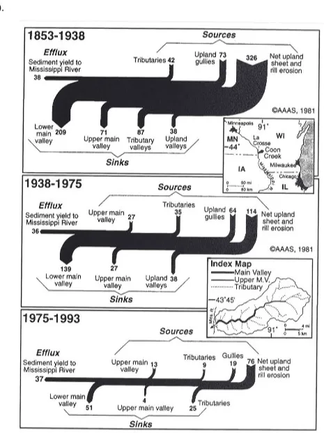
Figure 3.1: Sediment budgets for Coon Creek, a 360 km2 catchment in Wisconsin, USA, over the period 1853-1993. 'Numbers are annual averages in 103 Mg year-1. All values are direct measurements except "Net upland sheeet and rill erosion," which is the sum of all sinks and the efflux minus the measured sources. The lower main valley and tibutaries are sediment sinks, whereas the upper main valley is a sediment source' (Trimble, 1999,

modified from Trimble, 1981). 35

Figure 3.2: Sediment budget outline for low-lying sugarcane land. 39 Figure 4.1 (next page): Aerial photo of the study area for the sediment budget

study. The boundary of the cultivated lowland is indicated in red. 42 Figure 5 .1: Scatter diagram of turbidity versus SSC for all drain water samples

taken in the Ripple Comer Catchment. Both budget seasons plotted separately. Also shown are linear regression curves for each data set. 54 Figure 5.2: Profiles of cross-sections through Ripple Drain (a) and Prosser Drain

(b) at gauging sites. 55

Figure 5.3: Scatter diagram of Ripple Drain Dataflow depth data versus Starflow

depth data and a linear regression curve for 99-00 season. 57

Regression curves for Starflow depth data (99-00 data thick, 0 0-0ldata

thin). 60

Figure 5 .5: Ratios between manual velocity measurements as observed along the Ripple Drain surface profile and Starflow velocity as measured in the

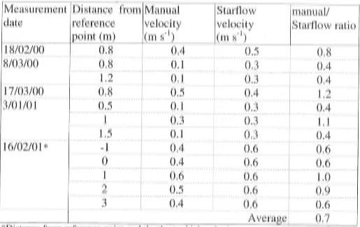
deepest part of the drain. 64

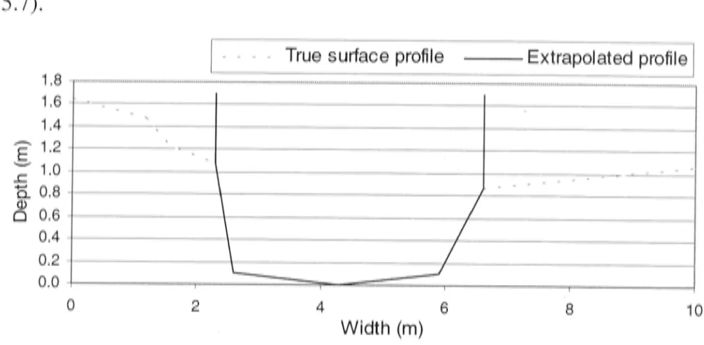
Figure 5 .6: Ratios between manual velocity measureme:Q.ts as observed along the Prosser Drain surface profile and Starflow velocity as measured in the deepest part of the drain. Inaccurate 16/02/01 estimates plotted separately. 65 Figure 5.7: Profile of cross-sections through Ripple Drain with vertically

extrapolated banks, used for discharge calculation during flood conditions. 67 Figure 5.8: Scatter diagram of Greenspan turbidity records versus grab sample

Turbiquant turbidity and SSC, with regression curve for Turbiquant turbidity. All samples taken from Ripple Drain gauging site during the

99-00 season. 68

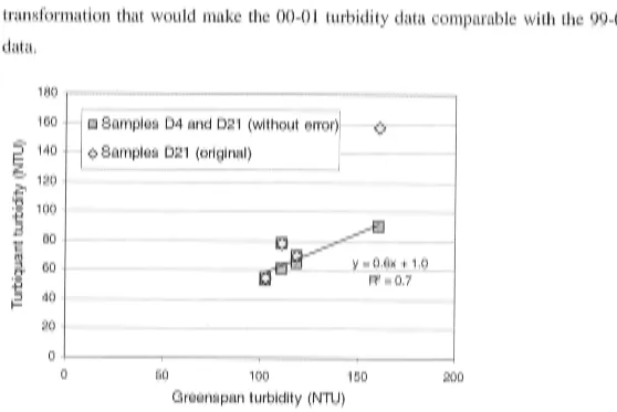
Figure 5.9: Scatter diagram of Greenspan versus Turbiquant turbidity data, for grab samples taken at Ripple Drain gauging site (D21) (with and without) and at Palmas' site (D4) in the 00-01 season. Regression curve for D4 and

D12 samples (without erroneous sample) included. 69

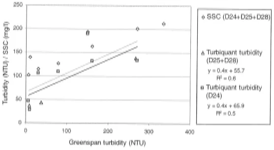
Figure 5 .10: Scatter diagram of Greenspan turbidity versus Turbiquant turbidity and SSC for grab samples taken at Prosser Drain gauging site (D24) and downstream locations in Prosser Drain (D25+D28) in the 99-00 season. Regression curves for Turbiquant data from locations D24 (thick) and

D25+D28 (thin) included. 70

Figure 5 .11: Scatter diagram of Greenspan turbidity versus Turbiquant turbidity and SSC for grab samples taken at the Prosser Drain gauging site in the 00-01 season. Regression curve for turbidity data included. 72 Figure 5.12: Scatter diagram of Ripple Drain depth versus Ripple Drain

discharge for both budget seasons. 00-01 data plotted both with and without

suspect data records. 74

Figure 5.13: Scatter diagram of Ripple Drain depth versus Ripple Drain velocity

for the 99-00 budget season. 7 4

Figure 5.14: Scatter diagram of Prosser Drain depth versus Prosser Drain

discharge for both budget seasons, unadjusted data. 76

Figure 5 .15: Scatter diagram of Prosser Drain depth versus Prosser Drain discharge for both budget seasons. Data adjusted for errors. 76 Figure 5.16: Scatter diagram of Ripple Drain depth versus Prosser Drain depth

for both budget seasons, unadjusted data. 78

Figure 5.17: Scatter diagram of Ripple Drain velocity versus Prosser Drain

velocity for both budget seasons. 78

Figure 5.18: Scatter diagram of Ripple Drain depth versus Prosser Drain depth for both budget seasons and a regression curve for the 99-00 data. Data

adjusted for errors. 79

Figure 5 .19: Scatter diagram of 99-00 Ripple Drain depth versus SSC. 81 Figure 6.1: Profile of cross-section through Post Creek at gauging site

(December 2000). 8 8

Figure 6.2: Relationship between Prosser Drain depth and Post Creek depth data for both budget seasons, and different Post Creek depth adjustments. 92 Figure 6.3: Post Creek depth- discharge rating curve (n=4, P=0.08). 93 Figure 6.4: Scatter diagram Rainfall versus Post Creek Discharge for both budget

seasons (n=196, P<0.01). 94

Figure 6.5: Scatter diagram of Turbidity versus SSC for Post Creek water samples and all Ripple Comer Catchment water samples (n=l0 and n=261). 95 Figure 6.6: Scatter diagram for Post Creek turbidity versus SSC for both budget

seasons (n=l0 and n=3, P=0.09). 95

Figure 6. 7: Calibration of Post Creek Greenspan turbidity probe with Turbiquant grab sample turbidity estimates and SSC estimate~ for both budget seasons

(n=6 and n=3, P<0.01). ₉₆

Figure 6.8: Regression curves Rainfall and Post Creek SSC for both budget

seasons (n=488, P<0.01). ₉₇

Figure 6.9: Scatter diagram of Post Creek Depth versus SSC for both budget

seasons. ₉₈

Figure 7.1: Set up of Parshall flume at the ratoon field site (side view). 104 Figure 7.2: Gauging data, south flume (2 - 5 April 1999). 106 Figure 7.3: Gauging data, south flume (15 - 19 March 2000). 106 Figure 7.4: Depth - discharge rating curve based on 99-00 south flume data.

(n=189, P<0.01) ₁₀₇

Figure 7 .5: Relationship between Ripple Drain water levels and south flume water depth (separate regression equations for RD depths <1.0 m (n=429,

P<0.01) and >1.0 m (n=58, P<0.01)) 108

Figure 7.6: Suspended sediment concentration - water depth relationship for the south flume. Samples for each season and the first event of each season

shown separately (n=78). ₁₀₉

Figure 7.7: Set up of cutthroat flumes at the plant cane site. 112 Figure 7.8: Plant flume gauging data (13 - 21 February 2001). 114 Figure 7.9: South flume and Plant flume depth and SSC data (13-21 February

2001). ₁₁₅

Figure 7.10: Scatter diagram of Ripple Drain (RD) versus plant flume (PF) water

depth data (n=229, P<0.01). ₁₁₆

Figure 7 .11: Depth - discharge rating curve based on 00-01 plant flume (PF)

data (n=247, P<0.01). ₁₁₆

Figure 7 .12: Suspended sediment concentration - water depth relationship for the south flume and plant flume. Samples for each season shown separately. 118 Figure 7 .13 Suspended sediment concentration - water depth relationship for

plant flume water depths >20 µm (n=75). 118

Figure 8 .1: Box plots for the variation in erosion rate, deposition rate and net surface level change on headlands during the 99-00 season, grouped by soil

type. ₁₃₀

Figure 8.2: Boxplots for the variation in erosion rate, deposition rate and net surface level change on headlands during the 99-00 season, grouped by crop

type. ₁₃₁

Figure 8 .3: Box plots for the variation in erosion rate, deposition rate and net surface level change on headlands during the 99-00 season, grouped by

drain type. ₁₃₂

Figure 8.4: Boxplots for the variation in erosion rate, deposition rate and net surface level change on headlands during the 00-01 season, grouped by soil

type. ₁₃₄

Figure 8.5: Boxplots for the variation in erosion rate, deposition rate and net surface level change on headlands during the 00-01 season, grouped by

Figure 8.6: Histograms of erosion rate (a), deposition rate (b ), and net surface level change ( c) of all 99-00 pinplots from the Ripple Comer Catchment. 137 Figure 8.7: Histograms of the erosion rate (a) and deposition rate (b) of the

logtransformed 99-00 pinplot data. 138

Figure 8.8: Scatter diagram of vegetation cover percentage and net surface level change (mm), with separate regressions for the 99-Q0 and 00-01 data (n=13,

P=0.09, and n=6, P<0.01). ₁₃₉

Figure 8.9: Headland along a plant cane (foreground right) and fallow (background) field. The headland section along plant cane is covered with sediment derived from the field after a heavy rainstorm in November 1999. The sediment buried the vegetation (see also inset; measuring-tape indicates

50 cm). ₁₄₃

Figure 8.10: Spatial distribution of net surface level change on pinplots J and M

between measurement sessions during the 99-00 season. 144

Figure 9 .1: Signs of soil erosion in different drain types in the Ripple Creek Catchment; results from the Integrated Drainage Survey (Roth et al., 2000). 149 Figure 9 .2: Schematic representation of the surface profile meter. 151 Figure 9 .3: Example of a surface profile through a water furrow in a ratoon field

on grey sand (profile 1). 156

Figure 9 .4: Box plots for the variation in erosion rate, deposition rate and net surface level change (original data) in different drain types (and water

furrows) during the 99-00 season. 158

Figure 9 .5: Boxplots for the variation in erosion rate, deposition rate and net surface level change (original data) in different drain types (and water

furrows) during the 00...:0l season. 159

Figure 9.6: Net surface level change in the original 99-00 drain profile data,

grouped by soil type (silty clay, clay and grey sand). 160

Figure 9. 7: Net surface level change in the original 00-01 drain profile data,

grouped by soil type (silty clay, clay and grey sand). 161

Figure 9. 8: Box plots for the variation in erosion rate, deposition rate and net surface level change (original data) in water furrows, grouped by soil type

(99-00 season). ₁₆₃

Figure 9.9: Boxplots for the variation in erosion rate, deposition rate and net surface level change (original data) in water furrows, grouped by soil type

(00-01 season). ₁₆₄

Figure 9.10: Boxplots for the variation in erosion rate, deposition rate and net surface level change (original data) in water furrows, grouped by crop type

(00-01 season). ₁₆₅

Figure 10.1: Particle size distribution of soil surface samples ( <10 cm) taken from headlands along Ripple Drain (HRD), _{major drains (HMaj) and minor}

drains (HMin). ₁₇₄

Figure 10.2: Sediment size distribution of soil surface samples ( <10 cm) from

fields (FG = grey sand, FS = silty clay, FC = clay) 176

Figure 10.3: Particle size distribution of soil surface samples ( <10 cm) taken from the beds of Ripple Drain (DRD) and major drains (DMaj). Sandy top layer ( <5 cm) at site DMaj6 is analysed separately. 177 Figure 10.4: Comparison of (Input - Storage) with catchment Output, showing

budget difference, for each budget calculation method. 183

Figure 10.5: Input of sediment from individual landscape elements for each

year's budget. ₁₈₅

Figure 10.6: Storage of sediment in individual landscape elements for each year's

budget. ₁₈₆

Figure 10.7: Net input of sediment from individual landscape elements. Positive values indicated net sediment storage, negative values net erosion. 186 Figure 11.1: Histogram of the absolute differences (deviations) between repeated

measurements of erosion pins in pin plot G in the 0Q-01 season. 194 Figure 11.2: Histogram of headland widths measured in the Ripple Comer

Catchment. ₁₉₆

Figure 11.3: Histogram of 1000 samples taken from a triangular distribution for

% _{particles <20 µm in headland surface soil. 197}

Figure 11.4: Cumulative frequency distribution curves obtained from 1000 simulations of headland sediment load, by re-sampling the original surface level change data (dark) and sampling from a normal distribution (light). Load estimates based on average and median surface level change data

indicated with dots. ₁₉₈

Figure 11.5: Worst case uncertainty estimates for headland sediment load calculations. Total range' shows the effect of assuming minimum and maximum values for all uncertainties. The separate effect of uncertainty in surface level change (SLC), surface area, measurement error, particle size

and bulk density is also shown. ₁₉₉

Figure 11.6: Worst case uncertainty estimates for catchment output calculations. 'Total range' shows the effect of assuming minimum and maximum values for all uncertainties. The separate effect of uncertainty in SSC,

cross-section, velocity and rating curve. ₂₀₃

Figure 11. 7: Worst case uncertainty estimates for the 99-00 sediment budget. 'Total range' (dark bars) shows the effect of assuming minimum and maximum values for all uncertainties. Light bars show separate effect on total sediment load of uncertainty in surface level change (SLC), surface area, measurement error, particle size and bulk density. 206 Figure 11.8: Cumulative frequency distribution curves obtained from 1000

simulations of the sediment budget components I-S (dark) and O (light). Best estimate values for each component are indicated with dots. 207 Figure 13 .1: Scenarios of erosion and deposition processes under four different

(flood) flow conditions on the Ripple Creek floodplain. ₂₂₅ Figure 13.2: SSC (mg

r

Comer Catchment (99-00 season). Dark bars indicate peak flow (backwater) conditions; Bright bars indicate free flow conditions. 226 Figure 13.3: Water depth (m), flow velocity (m s-1

) and SSC (mg

r

flow event in the Ripple Drain. Backwater effects cause reduction in flow velocity at greatest water depths. Dashed lines indicate times when water

samples were taken (7 and 10 February 2000). 227

Figure 13.4: Water and sediment discharge estimates for 6 sample dates on four locations in the Ripple Comer Catchment. Dark bars indicate peak flow (backwater) conditions; Bright bars indicate free flow conditions. 229 Figure 13.5: Clockwise hysteresis in the discharge - SSC relationship for the

peak flow event between February 4 and 12. Three minor flow events after

the main event are also included. ₂₂₉

Figure 14.1: Sediment budget diagram for the 1999-2000 wet season in the

PARTI

INTRODUCTORY CHAPTERS

Chapter 1

Introduction

1.1

_{Humid tropics and sugarcane cultivation}

Land use in the river catchments of tropical North Queensland appears to have increased the transport of sediment and nutrients to the coast. The increase is believed to threaten coastal and marine ecosystems as well as the freshwater ecosystems of the catchments. This thesis is focused on the transport of sediment in and from one type of land use in this region: sugarcane cultivation. A sediment budget is used to quantify rates of sediment production, deposition and export.

An outstanding feature of the North Queensland wet tropical coast is the concentration of high annual rainfall in a few months of the year; during this period several hundred millimetres of rain can fall within days or even hours. The intense rainfall causes large amounts of runoff and makes water levels in river drainage systems rise quickly. Because the rainstorms often persist for several days, flooding occurs frequently.

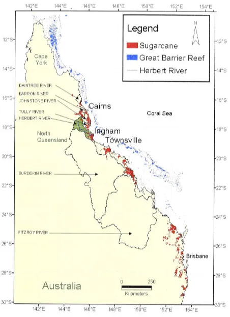
Large areas of sugarcane cultivation occupy the lowlands of North Queensland (Figure 1.1). Sugarcane crop needs 1500 mm of rainfall or irrigation each year and can survive under inundated conditions for several days. These characteristics make it a suitable crop for cultivation in the flood prone tropical lowlands. Production of sugarcane is now one of Australia's largest intensive agricultural industries. In the 2000-2001 season 424,350 hectares of cane was harvested (Canegrowers, 2002).

12°s 14°S 16°S 1s·s 20°s 22°s 24°S 26°S 28°S

142° E 144 °E

DAINTR EE RI VER

HERBERT RIVER

North Queensland

146°E

i.

i

I ~.

19' , ..,,,.

14 8° E 150° E 152°E

Legend

• sugar~ane

154°E

• Great Barrier Reef

- Herbert River

Coral Sea

· .. · _Tch,~~~~I_I~

·\ r.tgh,am

~

\

1 '-,, _~ . . , . ·• .. ~\ \

', . ' , ~~·

. ,. , l'>"'

. ---

..

,

"

BURDEl<IN RIVER _ _ _ ...,'I.J__._,,-• . ~~" ·, ,l~· -· _ . _.

,,.) ( ,. , ' • . :•a. _,;

~\ {~' 8\ ~

~-\

FITZROY RIVER - - - -~- ~ - ) ~ • ( }

~

~} ·,:i'!!

''i

.i-;. ·, Brisbane

' _·,:· q

Australia

3oos..,__ _ _ ~ -- - - - -- - ~ -- ---.-- ---.----'---.----'-300S 142°E 144 °E 146°E 148° E 1so0

E 152° E 154 °E

Figure 1.1: _{Map of North Queensland with sugarcane cultivation areas; seven of the major coastal}

catchments, including the Herbert River Catchment; and the Great Banier Reef.

Johnson et al. (2000) studied vegetation changes in the lower part of the Herbert River Catchment, the largest wet tropical catchment in North Queensland. They observed that the three key vegetation types in the original landscape, which are Eucalyptus dominated forest, Melaleuca (paper-bark) don1inated forest and Rainforest, have all been reduced, while the area under sugarcane has expanded. The highest loss was in the freshwater wetland Melaleuca communities (65 %). According to these authors , similar trends are apparent in other North Queensland catchments.

Introduction

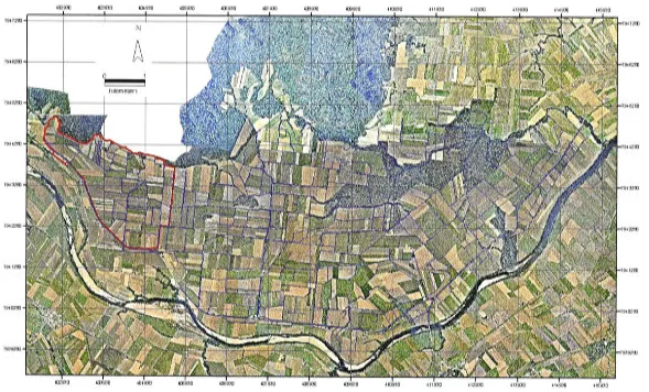
A second requirement to prepare country for cane growing is drainage of the cultivated surface. The natural landscape has very low relief and contains many depressions where water accumulates for some time after a flood. Creeks drain most of the lowland, but to remove the ponded water additional drainage lines are necessary. The high tropical rainfall is very welcome for the thirsty sugarcane crop, but prolonged waterlogging or inundation is not desirable because it reduces the cane yield (Cameron McNamara, 1980; Dick, 1982, in Herbert River Improvement Trust, 1993; R. Burry pers. comm.) and makes access to the fields with heavy 1nachinery difficult. Figure 1.2 shows an aerial photo of the Ripple Creek Catchment, a sub-catchment of the Herbert River, illustrating the typical cane land dissected by a dense network of drains (blue lines).

«:J:29JC 4'IJ9J• WHO• il05930 Ul5 9J• Wi'93• ID39J• ill39J• ,1093• , 1193• (1 293• '13930 ,H 9"JO '15 93•

i9( 72SJ + + ~ + +

-79 Hi2&J + I

-79( '28J

T9 Ul2'1J

i 9 Hl2&l

ICQ9J 0 ® 930 il[ligJ0 il059J0 Uli9J0 Ul79J• 0393• '°3930 l 109J• 41 1930 t 129J• '1J9J 0 4U9J0 '15930

Figure 1.2: _{Aeri al photo of Ripple Creek Catchment, a tributary of the Herbert Ri ver. Photo of}

fore sted upland section was not available. The (mostly artifi cial) drainage network in the catchment lowlands is highlighted in blue.

1.2

_{Increase in soil erosion since European settlement: the off-site}

effects

Introduction

in the intensively used areas (primarily the agricultural and urban zones) has been cleared or substantially modified (Cofinas and Creighton, 2001).

The human disturbance has a significant impact on the health of the landscape. Johnson et al. (2000) for example describe the vegetation changes in the lower part of the Herbert catchment as a 'decline of the diversity, quality, and integrity of the tropical lowland ecosystems'. Many researchers have also noticed how clearing and subsequent introduction of European style agriculture has led to severe degradation of the soil and increased erosion rates (yV _{asson and Galloway, 1986; Moss et al.,}

1992; Wasson et al., 1996). Large parts of the eroded material are redeposited elsewhere in the river catchments (Wasson et al., 1996), but a significant amount of sediment is exported to the catchment outlets, into the ocean. This has led to an increase of sediment, and associated nutrient, export to the coast from Australian river catchments. Moss et al. (1992) estimated a three to five-fold increase in sediment and nutrient export from the Queensland coastal catchments since European settlement.

On the land, degradation of the soil surface is not always recognized or acknow !edged as a problem. In certain areas the effects of increased sediment loads from rivers, have become the first reasons for concern. This is the case in tropical North Queensland (Rayment and Neil, 1996; Wasson, 1996). All coastal catchments in this region drain directly into the Great Barrier Reef World Heritage Area (GBRWH). The concern about potential impacts of the increased sediment loads from these catchments has been growing among scientists, government management agencies, and among the general population.

The Great Barrier Reef Marine Park occupies the Queensland coastal zone between the tip of Cape York and the Mary River near Hervey Bay, approximately 200 km north of Brisbane (Figure 1.1). The area contains the world's largest system of coral reefs (GBRMPA, 2001). It is best known for the astonishing coral reefs out in the ocean, but it also comprises many reefs closer to the shore, large areas of mangrove forest, and coastal wetlands. Increase in water turbidity is thought to harm coral reefs and more recently researchers have also become aware of the potential impact of sediments on coastal mangrove and freshwater wetland and river (eco) systems, which are important in the functioning of the Marine Park. The following section reviews the information upon which the concern is based.

Introduction

1.3

_{Effects of sediments and nutrients on the Great Barrier Reef}

World Heritage Area and riverine ecosystems

1.3.1 Increased sediment and nutrient inputs

CRC Reef Research Centre (2001) provides a concise overview of the current state

of know ledge on runoff from the land. On average 14 million tonnes of sediment,

49,000 tonnes of nitrogen and 9,000 tonnes of phosphorus are carried into the

GBRWH each year. This is a threefold increase of sediments and nitrogen over the

last 150 years and more than IO-fold for phosphorus. Slightly higher increases are

listed in the recent report by the Great Barrier Reef Marine Park Authority

(GBRMPA) (2001), which also states that the loads are still increasing without a sign

of abatement. A large part of the nitrogen ( 40%) and phosphorus (80%) carried by

the rivers is attached to fine sediment particles. River water concentrations of other

chemicals used in agriculture such as pesticides and their components ( e.g. Diuron,

atrazine, mercury and cadmium) are very low, but can accumulate in sediment

deposits and may have biological impacts (Bryan and Langston, 1992).

Over the last 15-20 years extensive research has been done to understand the

effects on the reef and coastal wetland systems of changes in runoff from the land.

Numerous reports have been published on this research by the involved organisations

(e.g. GBRMPA, Australian Institute for Marine Science (AIMS), CSIRO, etc.) and

regularly the findings are reviewed (Baldwin, 1990; Hillman, 1995; Crossland et al.,

1997; Hutchings and Haynes, 2000). The latest of such reviews are reported in

(GBRMPA, 2001; Williams, 2001; WWF, 2001).

1.3.2 Effects of sediment on coral reef systems

It _{is generally assumed that the increase of sediments, nutrients and other chemicals} will lead to increased degradation of coral reef systems (Wilkinson, 1999; Edinger et

al., _{1998). Sediments are seen as a potential threat to coral reef systems, but the exact}

effect of increased sediment loads is however still not very well understood. The

following reasons are given for concern about sediments.

They can exclude light from corals (Well-developed outer reef systems occur

only in seawater with low suspended particulate concentrations)

Introduction

- _{They can prevent the settlement of coral larvae on the reef surf ace}

Apart from direct threats there are possible indirect impacts, but their functioning is even less well known:

Crown-of-thorns (starfish) outbreaks may be related to increased phytoplankton

levels, caused by increased nutrient loads (partly associated with sediments) from

terrestrial runoff (Day, 2000)

- _{Changes in habitat due to reduction in micro-topography can have an indirect}

effect on the survival of corals

The scientific literature on all of these impacts is both limited and contradictory

(McClanahan and Obura, 1997; Williams, 2001; Marohasy and Johns, 2002).

Very recently some researchers have questioned the argument that higher

sediment loads increase turbidity of the seawater and cause the problems mentioned

above. Larcombe and Woolfe (1999) argue that turbidity levels and sediment

accumulation rates are at most coral reefs currently not limited by sediment supply.

Sediment input from rivers will not add significant extra turbidity to what is caused

by regular seabed disturbance already. They do note that the seaward terrigenous

sediment edges and coral reefs immediately adjacent to identified point sources of sediment input should be studied more closely.

Effects of sediment related chemicals

Besides impacts on coral reefs directly related to increased sediment concentrations in the seawater, there are problems caused by fertilizers and pesticides bound to particulate matter. Large amounts of these chemicals leave the land connected to soil particles and are transported into the ocean. When river water mixes with seawater

there is a possibility that they are released from the soil particles. Brodie and Mitchell (1992) found a significant proportion of inorganic Pin the flood plume of the Fitzroy River after mixing of the freshwater with seawater. The process of sorption and desorption of nitrogen and phosphorus from flood plumes into the seawater is however not sufficiently understood

Devlin and Taylor (1999) and GBRMPA (2001) list a number of observed

increases in chlorophyll concentrations in flood plumes and in water with sediment

resuspended by strong winds. Because phytoplankton and bacteria rapidly consume

nutrients in seawater, nutrient levels are typically low and a poor indicator of the

Introduction

nutrient status of reef water. Chlorophyll provides a better integrative measure of the amount of nutrients held' and cycling in the reef ecosystems. The increased

concentration among suspended sediment could indicate increased bioavailability of nutrients attached to sediments.

Cavanagh et al. _{(1999) failed to detect significant amounts of organochlorine in}

near-shore sediments, although easily detectable amounts were found in sugarcane

soils in the Herbert and Burdekin catchments, and the chemicals are known to move

attached to soil particles. There is no detectable organochlorine contamination of the GBRWH from historic agricultural activities in the catchments.

1.3.3 Effects of sediment on other marine ecosystems

Seagrass beds are important ecosystems in the GBRWH, situated in coastal areas

close to the input sources of terrestrial runoff. The beds can experience impacts from

sediment in direct and indirect ways similar to the coral reefs. Some research has shown that seagrass beds can die due to light deprivation as a result of increased turbidity (Preen et al., _{1995; Longstaff and Dennison, 1999). Potential impacts of}

nutrients are assumed, butno clear proof of negative impacts is available (Williams,

2001).

Many marine species rely on the coastal freshwater wetlands and mangroves as breeding and nursery areas (Robertson and Lee Long, 1991; GBRMPA, 2001).

Mixing between mangrove creek water and coastal seawater through tides ensures a strong dynamic link between mangroves and coastal waters (Wolanski et al., 1990),

making mangroves vulnerable to pollutants in the near shore waters. Trott and Alongi (1999) observed increased nutrient concentrations in mangrove creeks during

the summer wet season, which are probably due to erosion, solubilization and transport of nutrients from adjacent catchments into creeks. Negative impacts of the elevated nutrient levels were not noted.

1.3.4 Effects of sediments on freshwater ecosystems

Freshwater ecosystems also play an essential role in the functioning of the Great

Barrier Reef Marine Park. Many organisms, for example, use the fresh river water as breeding grounds. Because increased input of sediments and nutrients are routed

Introduction

There are several potential problems related to increased sediment loads in rivers (Arthington et al., _{1997). Suspended sediment causes water turbidity, which can}

diminish the light that is available for photosynthesis of stream vegetation, and decrease water temperature through increased reflection. Suspended material can also inhibit respiration and feeding of stream biota (Ryan, 1991).

Crossland (1999) points out that aquatic organisms in tropical rivers are well adapted to short term events with high concentrations of sediments and nutrients, because disturbance by floods is a normal occurrence in North Queensland streams. It _{is, however, a continuing supply of enhanced levels of nutrients and sediments} through the year via seepage, runoff, and irrigation tailwater that are likely to be of greater importance to aquatic communities.

1.3.5 Conclusion

The forgoing overview shows that there are potential direct and indirect impacts of increased sediment loads on many of the ecosystems of the GRBWH and the closely related freshwater systems. Firm evidence of a serious decline in any of the systems is however currently limited. This does not mean that terrestrial runoff can be ignored. Large-scale systematic studies on the GBRWH only started in the last 20 years or less and we do not know what the area looked like before European settlement. There are also studies from other parts of Australia and the rest of the world that indicate negative effects of sediments and nutrients on coral reefs and especially seagrass communities (Robertson and Lee Long, 1991; Edinger et al.,

1998; Corredor et al., _{1999). Similar effects could occur in the GBRWH and increase}

with continued or increasing inputs. Clearly most at risk are near-shore ecosystems such as near shore reefs and seagrass beds, because of their vicinity to the sites of sediment input.

A final very important concern is the potential cumulative effect of the increased (chronic and episodic) impacts of sediment pollution. Coral reefs and other ecosystems may be able to cope with impacts for a considerable time, but continued stress and unobserved sub-lethal effects can lead to fatal degradation in the longer term. Some studies worldwide have shown examples of systems that display such threshold effects (Williams, 2001).

Introduction

1.4

_{Soil erosion in low-lying sugarcane land}

Sugarcane land is mainly located in the low-lying areas of the North Queensland

catchments (see Figure 1.1). This industry is therefore situated adjacent to the many

coastal and freshwater ecosystems that play a role in th~ survival of the Great Barrier

Reef. The drainage water from the cane fields flows directly into these aquatic

ecosystems. During storm flows the drainage water has a 'dirty' colour, which

suggests that considerable amounts of sediments leave the catchment. Attached to the sediments will be fertilizers and pesticides that are used abundantly for cane

growing.

The only published research on soil erosion from cane land in Australia was done

on sloping cane land. In _{the Mackay region erosion rates in excess of 200 t ha-}1 _were

measured (Sallaway, 1979). Prove and Hicks (1991) observed values ranging from

50 to 500 t ha-1 _{on the wet tropical coast, where the magnitudes of erosion depended}

on rainfall amount and intensity, not soil type and slope. Although no numbers are available for erosion from low-lying cane land, their location close to the coast and the observations of sediment export through river water provide grounds for public

concern that sugarcane land is a major source of pollution. Even though decline of the Great Barrier Reef due to terrestrial runoff is not clearly demonstrated the sugarcane industry is often mentioned as, at least, a threat to the health of the Great

Barrier Reef (Flannery, 1994; WWF, 2001).

As a result of early observations of erosion, and signs of pollutants leaving the cane

lands, ameliorative action began in the 1980s (Prove and Hicks, 1991). Around that time Green Cane Trash Blanket (GCTB) harvesting was introduced in parts of the Queensland cane-growing region. This is a type of minimum-tillage harvesting,

where the leaves of the cane plant are left on the fields as trash cover after the harvest

of the cane stalks. GCTB harvesting now occurs in nearly 70% of the cane lands.

Prove et al. _{(1995) showed that the GCTB method reduces sediment runoff from}

sloping fields to levels comparable with those from rainforest, which were estimated at around 4 t ha-1 _{by Capelin and Prove (1983). Williams (2001) describes}

unpublished research on sediment cores from Hinchinbrook Channel and Missionary