Developing an imaging bi-spectrometer for fluorescent materials

(1)

Rochester Institute of Technology

RIT Scholar Works

Theses Thesis/Dissertation Collections

2-23-2009

Developing an imaging bi-spectrometer for

fluorescent materials

Mahnaz Mohammadi

Follow this and additional works at:http://scholarworks.rit.edu/theses

This Dissertation is brought to you for free and open access by the Thesis/Dissertation Collections at RIT Scholar Works. It has been accepted for inclusion in Theses by an authorized administrator of RIT Scholar Works. For more information, please [email protected].

Recommended Citation

(2)

Developing an Imaging Bi-Spectrometer for Fluorescent Materials

By

Mahnaz Mohammadi

B.S., Amirkabir University of Technology, Tehran, Iran (1993) M.S., Amirkabir University of Technology, Tehran, Iran (1996)

A dissertation submitted in partial fulfillment of the requirements for the degree of Doctor of Philosophy in the Chester F. Carlson Center for Imaging Science

Rochester Institute of Technology

February 23, 2009

Signature of Author _________________________________________________

(3)

CHESTER F. CARLSON CENTER FOR IMAGING SCIENCE ROCHESTER INSTITUTE OF TECHNOLOGY

ROCHESTER, NEWYORK

CERTIFICATE OF APPROVAL

Ph.D. DEGREE DISSERTATION

The Ph.D. Degree Dissertation of Mahnaz Mohammadi has been examined and approved by

the dissertation committee as satisfactory for the dissertation required for the

Ph.D. degree in Imaging Science

Dr. Roy S. Berns, dissertation Advisor

Dr. Mark D. Fairchild

Dr. Andreas Langner

Dr. Joseph Hornak

(4)

DISSERTATION RELEASE PERMISSION ROCHESTER INSTITUTE OF TECHNOLOGY

CHESTER F. CARLSON CENTER FOR IMAGING SCIENCE

Title of Dissertation

Developing an Imaging Bi-Spectrometer for Fluorescent Materials

I, Mahnaz Mohammadi, herby grant permission to Wallace Memorial Library of R.I.T. to reproduce my thesis in whole or in part. Any reproduction will not be for commercial use or profit

(5)

Developing an Imaging Bi-Spectrometer for Fluorescent Materials

BY

Mahnaz Mohammadi

Submitted to the

Chester F. Carlson Center for Imaging Science in partial fulfillment of the requirements

for the Doctor of Philosophy Degree at Rochester Institute of Technology

Abstract

Fluorescent effects have been observed for thousands of years. Stokes, in 1852, began the science of fluorescence culminating in his law of fluorescence, which explained that fluorescence emission occurs at longer wavelengths than the excitation wavelength. This phenomenon is observed extensively in the art world. Daylight fluorescent colors known as Day-Glo! have become an artistic medium since the 1960s. Modern artists exploit

these saturated and brilliant colors to glitter their painting.

Multipsectral imaging as a noninvasive technique has been used for archiving by

museums and cultural-heritage institutions for about a decade. The complex fluorescence phenomenon has been often ignored in the multispectral projects. The ignored

fluorescence results in errors in digital imaging of artwork containing fluorescent colors. The illuminant-dependency of the fluorescence radiance makes the fluorescence

colorimetry and consequently spectral imaging more complex.

In this dissertation an abridged imaging bi-spectrometer for artwork containing both fluorescent and non-fluorescent colors was developed. The method developed included two stages of reconstruction of the spectral reflected radiance factor and prediction of the fluorescent radiance factor. The estimation of the reflected radiance factor as a light source independent component was achieved by imaging with a series of

(6)

system for spectral imaging of paintings containing both fluorescent and non-fluorescent colors. The abridged two-monochromator method could predict fluorescent radiance factor of a fluorescent color via prediction of the true emission and the number of absorbed quanta by a fluorescing specimen for a given viewing light source. The superiority of the abridged fluorescence spectral imaging to the traditional spectral and colorimetric imaging for a few light sources was confirmed using fluorescent and non-fluorescent targets. Additionally, an exploratory visual experiment using a paired-comparison method was performed to evaluate the performance of the abridged

(7)

ACKNOWLEDGMENTS

To my advisor, Dr. Roy S. Berns, for his support and guidance in this dissertation and my graduate work. His advice and careful guidance were invaluable.

To my committee members, Dr. Mark Fairchild, Dr. Andrew Langner, and Professor Joseph Hornak for serving my thesis committee and their thoughtful advise through reading my dissertation.

To my professors at RIT for teaching me and sharing their precious knowledge.

To Mr. Lawrence Taplin for his enormous support for this dissertation and my graduate work.

To my dear husband and colleague, Dr. Mahdi Nezamabadi, for his unlimited support during my graduate work.

To Mrs. Valerie Hemink and Mrs. Collen Desimone for assisting me with the administrative tasks during my graduate life at RIT.

To the staff and students at Munsell Color Science Lab and Center for Imaging Science at RIT for their friendship, kindness, and encouragement during my graduate work and participating in my visual experiments.

To Mr. Michael Goodwin at Kodak for providing the fluorescent measurement instrument.

To Mrs. Azin Mohammadi for helping me in sample preparation.

To Mrs. Zohreh Lotfabadi, Mrs. Curtice and Dr. Franziska Fray for drawing wonderful paintings.

To Mr. Shozhe Shen for helping me in running my visual experiment.

To the RIT writing service staff for editing my dissertation.

To my dear parents, Sedigeh Vahdai and Esmaeil Mohammadi for their encouragements, support, and patience during my long years of education.

(8)

To my dear son, Navid Nezamabadi, for his love and patience while I was working on my PhD program.

(9)

DEDICATION

(10)

4 Prediction of Fluorescence Emission, A New Model... 52

4.1 Introduction ... 52

4.2 Principles of Fluorescence Emission ... 57

4.2.1 True Emission and the Number of Absorbed Quanta ... 58

4.2.2 Abridged Two-Monochromator Method... 61

4.3 Implementation of the Abridged Two-Monochromator Method ... 67

4.3.1 Exploratory Experiment ... 67

4.4 Results and Discussions ... 73

5 Abridged Fluorescence Spectral Imaging... 90

5.2 Filter-Based Abridged Fluorescence Reduction Methods ... 94

5.3 Simulation of Filter Fluorescence Reduction Imaging... 99

(11)

5.3.4 Virtual Camera... 108

5.3.5 A Numerical Example... 113

5.3.6 Results and Discussion... 122

6 Image-Based Abridged Fluorescence Spectral Imaging ... 140

6.2 Image-Based Filter Fluorescence Reduction Spectral Imaging ... 142

6.2.1 Light source ... 142

6.2.2 Calibration and Verification Targets... 144

6.2.3 Image Acquisition System... 146

6.2.4 Geometry of Imaging ... 152

6.2.5 Results and Discussion... 153

6.3 Prediction of the Spectral Fluorescent Radiance Factor... 168

6.3.1 UV-Fluorescence Imaging... 171

6.3.2 Creating a Weighted Donaldson Luminescence Matrix... 183

6.3.3 Calculating an Abridged Donaldson Luminescence Matrix ... 186

6.3.4 True emission... 190

6.3.5 Prediction of the Number of Absorbed Quanta ... 194

6.4 Prediction of the Total Radiance Factor ... 198

6.5 Fluorescence, Spectral, and Colorimetric Imaging ... 207

7 Visual Evaluation of the Imaging Models... 239

7.1 Viewing Light Sources ... 240

7.2 Display Characterization... 241

7.3 Adjusting light booth and LCD ... 245

7.4 Stimuli Preparation ... 246

7.5 Paired-Comparison Experiment ... 254

7.6 Results and Discussion ... 257

8 Summary and Conclusions... 265

8.1 Scientific Contributions ... 273

8.2 Future Study ... 275

9 Bibliography ... 276

(12)

List Of Figures

Figure 2.1 Examples of artwork containing fluorescent colors...9

Figure 2.2 Example of a painting containing both fluorescent and non-fluorescent colors

under daylight and incandescent A. ... 12

Figure 2.3 A flowchart of abridged fluorescence spectral imaging... 16

Figure 3.1 The Donaldson radiance factor matrix for Golden!_{fluorescent orange}

measured by a bispectrometer, a Labsphere BFC-450... 21

Figure 3.2 Fluorescence and excitation spectra of Golden! fluorescent orange based on

the abridged Donaldson luminescence radiance factor measured by a Labsphere

BFC-450 (wavelength interval in 50 nm.)... 24

Figure 3.3 Calculated excitation spectra of Golden"_{fluorescent orange under CIE}

illuminant D65 (green line) and CIE illuminant A (red line) using the measured

Donaldson luminescence radiance factor with Labsphere BFC-450, and spectral

excitation factor (blue line)... 28

Figure 3.4 Excitation and emission spectra of a white fluorescent sample showing the

overlap between the two, Grum (1980). ... 29

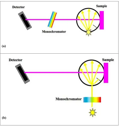
Figure 3.5. A schematic design of the components of a reflectance spectrophotometer

employing polychromatic irradiation, (a) and monochromatic irradiation and

polychromatic detection (b). ... 31

(13)

heavy lines indicate the reflectance measured through each of these filters: $1, $2, $3,

(Billmeyer 1979). ... 33

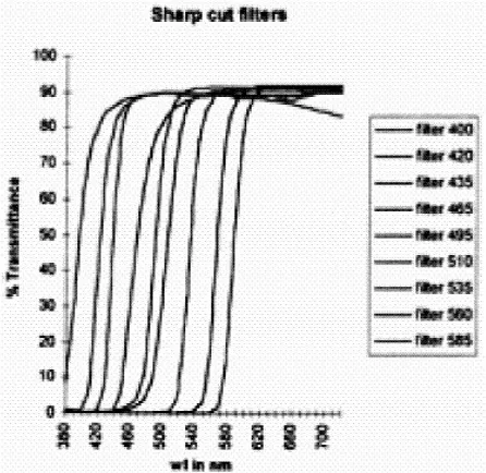
Figure 3.7 Transmission of serial short-wavelength cutoff filter set used in serial filter

method proposed by Simon (1998). ... 34

Figure 3.8. Calculation data for a Blaze orange sample. The heavy lines indicate total

radiance factor, %T, reduced total radiance factor, %&T, and reflectance, $. The thinner

lines indicate the transmittance curves of the fluorescence-reducing filter, #1, and the

transmittance of the fluorescence-killing filter, #2, (Billmeyer 1979)... 37

Figure 3.9 The two-mode method applied to a Blaze orange sample (Billmeyer 1979). . 38

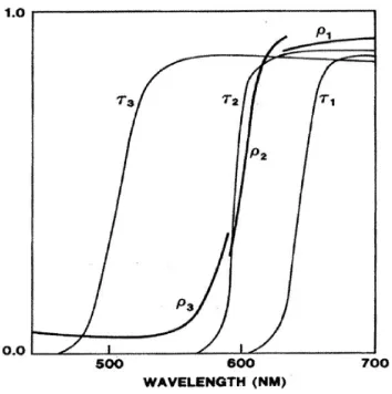
Figure 3.10 Total radiance factor (1), reflected radiance factor (2), and conventional

reflectance (3) of a green fluorescent sample. Vertical lines denote the excitation

region, Grum and Costa (1977)... 44

Figure 3.11. Relative radiant power distributions of 10 different phases of daylight

obtained in accordance with CIE method of calculating daylight illuminants for

colorimetry (Wyszecki 1964)... 46

Figure 3.12. High quality D65 simulator based on Xenon lamp, compared with D65 and

Illuminant ID65, representing interior daylight (Clarke 1982)... 47

Figure 3.13 Spectral radiance factor of Arc Yellow measured on the seven commercial

(14)

Figure 4.1 Calculated fluorescence emission of Golden" fluorescent orange upon

excitation with excitation wavelengths below 560 nm using the measured Donaldson

luminescence radiance factor matrix. ... 59

Figure 4.2 Calculated fluorescence emission of Golden"_{fluorescent orange under CIE}

illuminant D65 (green line) and CIE illuminant A (red line) using the Donaldson

luminescence radiance factor matrix measured with a Labsphere BFC-450, and true

emission (blue line). ... 61

Figure 4.3 A Flow chart of predicting the fluorescence emission based on the abridged

two-monochromator method... 62

Figure 4.4 Relative spectral power distribution of CIE illuminant D65, A, and D50

normalized at 560 nm. ... 69

Figure 4.5 Normalized fluorescence emission spectra of the fluorescent paints calculated

based on the measured Donaldson luminescence radiance factor matrix with a

Labsphere BFC-450 under UV excitation wavelengths. ... 70

Figure 4.6 Excitation (red line) and fluorescence emission (green line) spectra of the six

Golden! fluorescent paints measured with a Labsphere BFC-450... 71

Figure 4.7 True emission spectra. The blue line represents the calculated true emission

using the measured Donaldson luminescence radiance factor matrix with a

Labsphere BFC-450 and the green line is the predicted true emission based on the

(15)

Figure 4.8 Overall Predicted and actual number of absorbed quanta of the fluorescent

colors under different initial and viewing illuminants. The actual values are based on

the measured Donaldson luminescence radiance factor matrix with a Labsphere

BFC-450 and the predicted values are based on the abridged two-monochromator

method. ... 76

Figure 4.9 Multiple comparison analysis on the mean of the error between the predicted

and actual number of absorbed quanta for models under different initial and viewing

illuminants... 79

Figure 4.10 Predicted and actual number of absorbed quanta of the fluorescent colors

under different initial and viewing illuminants. The actual values are based on the

measured Donaldson luminescence radiance factor matrix with a Labsphere

BFC-450 and the predicted values are based on the abridged two-monochromator method.

... 81

Figure 4.11 Fluorescence emission spectra under CIED65 using different initial

illuminants. Cyan line represents the calculated emission under CIED65 using the

BFC-450. ... 85

Figure 4.12 Fluorescence emission spectra under CIEA using different initial illuminants.

Cyan line represents the calculated emission under CIEA using the measured

(16)

Figure 4.13 Fluorescence emission spectra under CIED50 using different initial

illuminants. Cyan line represents the calculated emission under CIED50 using the

BFC-450. ... 87

Figure 5.1 Spectral fluorescence emission (green line) and excitation (cyan line) spectra

of Golden! acrylic fluorescent orange. The red and the blue lines are the spectral

transmittance factor of the fluorescence-weakening and fluorescence-killing filters,

respectively. ... 95

Figure 5.2 Total radiance factor of Golden! acrylic fluorescent orange with and without

excitation filters; the blue line is without the filter, the red line is with the

fluorescence-weakening filter, and the green line is with the fluorescence-killing

filter. ... 97

Figure 5.3 Total radiance factor of Golden! fluorescent orange under CIE illuminant

D65 and A using the measured Donaldson luminescence radiance factor matrix by a

Labsphere BFC-450... 101

Figure 5.4 Spectral transmittance factor of short-wavelength cutoff filters used in filter

fluorescence reduction spectral imaging. The blue solid line is Rosco 312 and the

others are Lee filters (top left plot). The spectral transmittance factor of the

sandwich of the filters with Rosco 312. Blue solid line is Rosco 312 and the others

(17)

Figure 5.5 The relative spectral power of CIE illuminant A (the solid blue line) and the

new illuminants simulated by inserting the short-wavelength cutoff filters in the

excitation path in order tabulated in Figure 5.4. ... 104

Figure 5.6 The ‘CCFL’ calibration target. The spectral reflected radiance factor of the

‘Fluor chart 1’ (left) and GretagMacbeth Color Checker (right) measured by a

Labsphere BFC-450 and a SpectroEye 45/0, respectively. ... 106

Figure 5.7 Representation of the fluorescent and non-fluorescent colors employed in the

simulation fluorescence reduction imaging. ... 108

Figure 5.8 Relative spectral sensitivity of modified Sinarhack 54. The blue, green, and

red lines represent the sensitivity of the blue, green, and red channels. The solid

lines correspond to the Schott filter GG475 and the dashed line represents the

sensitivity of the camera with Schott filter BG39. The sensitivity plots were

normalized in respect to the global maximum sensitivity. ... 110

Figure 5.9 The best average spectral RMS% error between the reconstructed reflected

radiance factor based on filter fluorescence reduction spectral imaging and the

measured reflected radiance factor by a Labsphere BFC-450. Calibration target was

the ‘CCFL’. ... 125

Figure 5.10 Spectral reflected radiance factor of the Fluor Chart1’. The green line is the

reflected radiance factor measured by a Labsphere BFC-450 and the red line

(18)

fluorescence reduction spectral imaging with three light sources. Calibration target

was the ‘CCFL’. ... 129

Figure 5.11 Spectral reflected radiance factor of the ‘Fluor Chart2’. The green line is the

measured by a Labsphere BFC-450 and the red line represents the reconstructed

reflected radiance factor based on simulation filter fluorescence reduction spectral

imaging with three light sources. Calibration target was the ‘CCFL’... 130

Figure 5.12 Spectral reflected radiance factor of a GretagMacbeth Color Checker (CC).

The green line is the measured reflected radiance factor by a GretagMacbeth

SpectroEye and the red line represents the reconstructed reflected radiance factor

based on simulation filter fluorescence reduction spectral imaging with three light

sources. Calibration target was the ‘CCFL’... 131

Figure 5.13 Difference between the predicted and measured reflected radiance factors of

the GretagMabeth ColorChecker (CC) and GretagMabeth ColorChecker DC

(CCDC). The left and right plots correspond to prediction values based on a

single-illuminant and three-single-illuminant imaging system, respectively. The calibration target

was GretagMabeth ColorChecker (CC)... 135

Figure 6.1 The measured spectral power distribution of Broncolor Pulso G

(tungsten-based), blue line, and the generated lights sources using Broncolor Pulso G

(tungsten-based) plus the short-wavelength cutoff filters in the excitation path. ... 143

(19)

Figure 6.3 Pictures of a scene illuminated by Broncolor Pulso G (tungsten-based) filtered

by Rosco 312 (left) and a sandwich of Rosco 312 and Lee 113 (right). ... 144

Figure 6.4 The ‘Calib FRS1’. The spectral reflected radiance factor of the ‘Fluor Chart1’

in left site and the Esser Test Chart TE221 in the right site. ... 145

Figure 6.5 A modified Sinarback 54 digital camera. ... 147

Figure 6.6 The captured image of a GretagMacbeth Color Checker (CC) under Broncolor

Pulso G with a Sinarback 54 with two camera-filters with the same exposure time.

Left and right images were captured with Schott BG39 and Schott GG475 filters,

respectively. ... 147

Figure 6.7 A flowchart of image preparation for the solid patches in spectral imaging

with a modified Sinarback 54. The symbol ‘m’ stands for the number of patches in

the target, ‘L’ represents the digital count, and the number 6 corresponds to the six

channels of the digital camera... 149

Figure 6.8 A transformation matrix, T, derived based on an imaging with a six-channel

spectral imaging under tungsten-based Broncolor Pulso G. The calibration target

was the ‘Calib FRS2’. The blue and green lines correspond to red channels under

Schott GG475 and BG39 filters. The red and cyan lines correspond to green

channels under Schott GG475 and BG39 filters. The magenta and yellow lines

correspond to blue channels under Schott GG475 and BG39 filters. ... 151

(20)

Figure 6.10 A picture of the experimental set up for filter fluorescence reduction spectral

imaging. ... 153

Figure 6.11 The average spectral RMS% error between the image-based reconstructed

reflected radiance factor based on filter fluorescence reduction spectral imaging and

the measured by a Labsphere BFC-450. The results correspond to the best

reconstruction performance for each target. The calibration target was the ‘Calib

FRS1’... 155

Figure 6.12 The spectral reflected radiance factors of the ‘Fluor Chart2’ in top and the

picture of this chart in bottom. ... 159

Figure 6.13 The average spectral RMS% error between the image-based reconstructed

and the measured reflected radiance factor with a Labsphere BFC-450. The results

correspond to the best reconstruction performance for each target. Calibration target

was the ‘Calib FRS2’... 160

Figure 6.14 Spectral reflected radiance factors of the ‘Mixed Chart’. Green line is the

measurement with a Labsphere BFC-450 and red line represents the image-based

reconstructed based on the filter fluorescence reduction spectral imaging.

Calibration target was the ‘Calib FRS1’... 162

Figure 6.15 Spectral reflected radiance factors of the ‘Mixed Chart’. Green line is the

(21)

Figure 6.16 Spectral reflected radiance factors of the ‘Fluor Chart1’. Green line is the

Figure 6.17 Spectral reflected radiance factors of the ‘Fluor Chart 2’. Green line is the

Figure 6.18 Spectral reflected radiance factors of a GretagMacbeth ColorChecker. Green

line is the measurement with a GretagMacbeth SpectroEye and red line represents

the image-based reconstructed based on filter fluorescence reduction spectral

imaging. Calibration target was the ‘Calib FRS2’. ... 167

Figure 6.19 Spectral reflected radiance factors of the Gamblin. Green line is the

measurement with a GretagMacbeth SpectroEye and red line represents the

image-based reconstructed image-based on filter fluorescence reduction spectral imaging.

Figure 6.20 The relative spectral power distribution of UV-A light source, Spectroline

XX-40. ... 172

Figure 6.21 An experimental set up for UV-imaging to reconstruct the fluorescence

(22)

Figure 6.22 Spectral radiances of the “Fluor Chart1” under a Spectroline XX-40 (UV-A

light source) measured by a Photo Research SpectroScan PR650. The Blue, green,

red, cyan, magenta, and yellow correspond to the radiance of blue, green, magenta,

orange, red, and yellow, respectively. ... 174

Figure 6.23 Spectral radiances of the illuminated Halon under UV-A light source and

measured by a Photo Research SpectroScan PR650. ... 175

Figure 6.24 The normalized spectral fluorescence curve of the “Fluor Chart1”. Green line

represents the predicted spectral fluorescence based on UV-fluorescence imaging

and the blue line shows the measured spectral fluorescence with a Labsphere

BFC-450. ... 178

Figure 6.25 The normalized spectral fluorescence curve of the “Fluor Chart2”. Green line

BFC-450. ... 179

Figure 6.26 The normalized spectral fluorescence curve of the “Mixed Chart”. Green line

BFC-450. ... 180

Figure 6.27 An example of a cubic spline function with parameters w1, w2, 'c ,h... 182

(23)

Figure 6.29 Total radiance factors of the “Fluor Chart2” under TL201 (green line) and

under Broncolor Pulso G (tungsten-based) measured with a Photo Research

SpectroScan PR650. ... 185

Figure 6.30 Total radiance factors of the ‘Fluor Chart2’ under TL201. Green line is the

estimated and blue line is the calculated based on the measured Donaldson radiance

factor matrix with a Labsphere BFC-450. Calibration target was the “CalibTotal”.

... 188

Figure 6.31 The predicted true emission of the “Fluor Chart1” based on the fluorescence

spectral imaging (green line) and the calculated true emission using the measured

Donaldson luminescence radiance factor matrix with a Labsphere BFC-450 (blue

line)... 192

Figure 6.32 The predicted true emission of the ‘Fluor Chart2’ based on the fluorescence

line)... 193

Figure 6.33 The predicted true emission of the ‘Mixed Chart’ based on the fluorescence

line)... 194

Figure 6.34 The predicted and actual number of absorbed quanta of the fluorescent colors

(24)

Donaldson luminescence radiance factor matrix with a Labsphere BFC-450 and the

predicted is based on the abridged two-monochromator method. ... 196

Figure 6.35 The predicted and actual number of absorbed quanta of the fluorescent colors

under daylight illumination. The actual value is based on the measured Donaldson

luminescence radiance factor matrix with a Labsphere BFC-450 and the predicted is

based on the abridged two- monochromator method. ... 197

Figure 6.36 Total radiance factors of the ‘Fluor Chart1’ under the simulated daylight

Spectralight II. The green line is the predicted based on fluorescence spectral

imaging and the blue line represents the calculated total radiance factor using the

measured Donaldson radiance factor matrix with a Labsphere BFC-450... 202

Figure 6.37 Total radiance factors of the ‘Fluor Chart2’ under the simulated daylight

imaging and the blue line represents the calculated total radiance factors using the

Figure 6.38 Total radiance factors of the ‘Mixed Chart’ under the simulated daylight

Figure 6.39 Total radiance factors of the ‘Fluor Chart1’ under the incandescent

(25)

Figure 6.40 Total radiance factors of the ‘Fluor Chart2’ under the incandescent

Spectralight II. The green line is the predicted based on the fluorescence spectral

Figure 6.41 Total radiance factors of the ‘Mixed Chart’ under the incandescent

Spectralight II. The green line is the predicted based on the fluorescence spectral

Figure 6.42 Difference between the predicted total radiance factors and the calculated

ones ones based on the measured Donaldson matrix with a Labsphere-BFC450. The

left plots are the difference corresponding to the simulated daylight and the right

plots correspond to incandescent viewing light source. The first row is for prediction

based on fluorescence spectral imaging and the second and third rows are prediction

under xenon- and tungsten -based spectral imaging, respectively... 214

Figure 6.43 Total radiance factor of the ‘Fluor Chart2’ under the simulated daylight

GretagMacbeth Spectralight II. The green line is the predicted based on the

fluorescence spectral imaging, the blue line represents the reconstructed based on

(26)

calculated total radiance factor using the measured Donaldson radiance factor matrix

with a Labsphere BFC-450. ... 216

Figure 6.44 Total radiance factor of the ‘Fluor Chart2’ under the simulated daylight

GretagMacbeth Spectralight II. The green line is the predicted based on the

fluorescence spectral imaging, the blue line represents the reconstructed based on

the xenon-based traditional spectral imaging, and the red line represents the

calculated total radiance factor using the measured Donaldson radiance factor matrix

with a Labsphere BFC-450. ... 217

Figure 6.45 Total radiance factor of the ‘Fluor Chart2’ under the incandescent

GretagMacbeth Spectralight II. The green line is the predicted based on fluorescence

spectral imaging, the blue line represents the reconstructed based on the

tungsten-based traditional spectral imaging, and the red line represents the calculated total

radiance factor using the measured Donaldson radiance factor matrix with a

Labsphere BFC-450... 218

Figure 6.46 A comparison of the average spectral RMSE% between the reference and

predicted spectral reflected radiance factors for the non-fluorescent targets. The

reference was the measurements with a GretagMacbeth SpectroEye. The predicted

reflected radiance factors were based on the different imaging models, xenon-based

spectral imaging (blue bar), tungsten-based spectral imaging (green bar), and

(27)

Figure 6.47 A multiple comparison on the mean of CIE !E00 for the CIE 1931 2º standard

observer of different models under the simulated daylight and incandescent viewing

light sources for all 41 (41 = 6 patches of the ‘Fluor Chart1’ + 14 patches of the

‘Fluor Chart2’ + 21 patches of the ‘Mixed Chart’) of the fluorescent colors... 227

Figure 7.1 Spectral power distribution of the simulated daylight and incandescent light

sources of the GretagMacbeth Spectralight II. Red line represents the simulated

daylight and the blue line is for the incandescent light source. ... 240

Figure 7.2 1-D LUTs for RGB channels of an Apple Cinema HD LCD... 244

Figure 7.3 Total radiance factor of six pure Golden! fluorescent paints for two viewing

light sources. The solid blue and dashed green lines represent the total radiance

factors under the simulated daylight and INCA, respectively. ... 246

Figure 7.4 A picture of the ‘House’ used in psychophysics experiment before touching

with non-fluorescent paints... 247

Figure 7.5 Flow chart of the abridged fluorescence spectral imaging. ... 249

Figure 7.6 Flow chart of fluorescence filter reduction spectral imaging to reconstruct the

reflected radiance factor image. ... 251

Figure 7.7 Flow chart of fluorescent radiance factor prediction for a given viewing light

source... 253

Figure 7.8 Set up of the psychophysical experiment. ... 255

Figure 7.9 Set up of psychophysical experiment showing the fluorescent radiance factor

(28)

Figure 7.10 Interval scales and the corresponding 95% confidence level based on the

paired comparison experiment for the simulated daylight as viewing light source.259

paired comparison experiment for the incandescent as viewing light source... 261

paired comparison experiment for the simulated daylight as viewing light source

after showing the fluorescent radiance factor image... 262

paired comparison experiment for the incandescent as viewing light source after

showing the fluorescent radiance factor image... 263

Figure 10.1 Rendered image of the House for the simulated daylight based on the

abridged fluorescence spectral imaging... 289

xenon-based spectral imaging... 290

xenon-based colorimetric imaging... 291

tungsten-based spectral imaging. ... 292

(29)

Figure 10.6 Rendered image of the House for the incandescent based on the abridged

fluorescence spectral imaging... 294

Figure 10.7 Rendered image of the House for the incandescent based on the xenon-based

spectral imaging. ... 295

Figure 10.8 Rendered image of the House for the incandescent based on the xenon-based

colorimetric imaging... 296

Figure 10.9 Rendered image of the House for the incandescent based on the

tungsten-based spectral imaging... 297

Figure 10.10 Rendered image of the House for the incandescent based on the

tungsten-based colorimetric imaging... 298

Figure 10.11 Rendered image of the ‘Fluor Chart2’ for the simulated daylight based on

the abridged fluorescence spectral imaging... 299

Figure 10.12 Rendered image of the ‘Fluor Chart2’ for the incandescent based on the

abridged fluorescence spectral imaging... 299

Figure 10.13 Rendered image of the ‘Mixed Chart’ for the simulated daylight based on

the abridged fluorescence spectral imaging... 300

Figure 10.14 Rendered image of the ‘Mixed Chart’ for the incandescent based on the

(30)

List Of Tables

Table 3.1 Total radiance factor values, Donaldson radiance factor matrix, for Golden!

fluorescent orange measured by a Labsphere BFC-450. (Values less than 0.01 have been set to zero.) ... 21 Table 3.2 A reflected radiance factor matrix corresponding to Donaldson matrix listed in Table 3.2 for Golden! fluorescent orange measured by a Labsphere BFC-450. ... 22

Table 3.3 A fluorescent radiance factor matrix corresponding to Donaldson matrix listed in Table 3.2 for Golden! fluorescent orange measured by a Labsphere BFC-450 (Values

less than 0.01 have been set to zero.) ... 23 Table 3.4 Mean percent deviations for different abridged methods from the

(31)

Table 5.10 A list of illuminants in two- and three- illuminants models that perform the best for each target. ... 127 Table 5.11 Statistical summary of the spectral RMS% error between the measured and reconstructed spectral reflected radiance factor based on the simulation fluorescence filter reduction spectral imaging with three light sources, (lights 1,2, and 5). Calibration

targets were the ‘CCFL’ and CC. ... 133 Table 5.12 Statistical summary of the spectral RMS% error between the measured and reconstructed spectral reflected radiance factor based on the simulation fluorescence filter reduction imaging for the non-fluorescent targets with different light sources and

calibration targets... 134 Table 6.1 Set up of experiment for imaging under different light sources with a modified Sinarback 54. ... 150 Table 6.2 RMSE% between the image-based reconstructed and measured reflected

radiance factors of the fluorescent and non-fluorescent targets. Calibration target was the ‘Calib FRS1’... 156 Table 6.3 A list of light sources used in filter fluorescence reduction spectral imaging to yield the best performance for different targets... 157 Table 6.4 The average spectral RMSE% between the image-based reconstructed and measured reflected radiance factor for different targets using different set of light sources. ... 158 Table 6.5 RMSE% between the image-based reconstructed and measured reflected

radiance factors of the fluorescent and non-fluorescent targets. Calibration target was the ‘Calib FRS2’... 161 Table 6.6 Statistical summary of spectral RMSE% between the predicted true emission based on the fluorescence spectral imaging and the calculated true emission using the measured Donaldson matrix with a Labsphere BFC-450... 191 Table 6.7 Statistical summary of spectral RMSE% between the predicted total radiance factor based on the fluorescence spectral imaging and the reference values calculated based on the measured Donaldson matrix with a Labsphere BFC-450. ... 199 Table 6.8 A summary of the specification of the imaging models. ... 209 Table 6.9 Statistical summary between the predicted and reference total radiance factors for a simulated daylight GretagMacbeth Spectralight II as a viewing light source. The reference was the total radiance factor based on the measured Donaldson matrix with a Labsphere BFC-450. The predicted total radiance factors corresponded to two different models, traditional and fluorescence spectral imaging. ... 211 Table 6.10 Statistical summary between the predicted and reference total radiance

(32)

reference was the total radiance factor based on the measured Donaldson matrix with a Labsphere BFC-450. The predicted total radiance factors corresponded to two different models, traditional and fluorescence spectral imaging. ... 212 Table 6.11 Statistical summary of reflected radiance reconstruction based on xenon-based and tungsten-based spectral imaging and fluorescence spectral imaging for the non-fluorescent colors. ... 219 Table 6.12 A statistical summary of colorimetric (CIE !E00, CIE 1931 2º standard

(33)

1

Terminology

The definitions in this chapter are based on the international terminology from

publication CIE No. 38 (TC-2.3), which were extracted from the Billmeyer report (1979)

without any changes, and ASTM E-284-03a (2004).

Abridged spectrophotometry. Measurement of reflectance factor or transmittance factor

in a number of wavelength bands rather than as continuous functions of wavelength.

Absorptance, Ratio of the absorbed radiant or luminous flux to the incident flux.

Bispectral radiance factor. Ratio of the spectral radiance (radiance per unit waveband)

at wavelength ' from a point on the specimen when irradiated at wavelength µ to the

total (integrated spectral) radiance of the perfectly reflecting diffuser similarly irradiated

and viewed (Symbol, b'(µ)).

Bispectral fluorescence radiance factor. Ratio of the spectral radiance at wavelength '

due to fluorescence from a point on the specimen when irradiated at wavelength µ to the

total radiance of the perfectly reflecting diffuser similarly irradiated and viewed (Symbol,

bF'(µ)).

Bispectral reflection radiance factor. Ratio of the spectral radiance at wavelength ' due

to reflection from a point on the specimen when irradiated at wavelength µ to the total

radiance of the perfectly reflecting diffuser similarly irradiated and viewed (Symbol,

(34)

Bispectrometer. An optical instrument equipped with a source of irradiation, two

monochromators, and a detection system, such that a specimen can be measured at

independently-controlled irradiation and viewing wavelengths. The bispectrometer is

designed to allow for calibration to provide quantitative determination of the bispectral

radiation-transfer properties of the specimen.

Color stimulus. A radiant flux capable of producing a color perception.

Color stimulus function )('). Description of a color stimulus by the spectral

concentration of a radiometric quantity, such as radiance or radiant power, as a function

of wavelength.

Conventional reflectometer value. Apparent reflectometer value when a fluorescent

material is measured relative to the (non-fluorescent) perfect reflecting diffuser, using a

reflectometer with monochromatic irradiation and polychromatic detection.

Daylight illuminant. An illuminant having the same, or nearly the same, relative spectral

power distribution as a phase of daylight (Symbol, $C).

Discrete bispectral radiance factor, B(',µ). A matrix defined for specified irradiation

and viewing bandpass functions, and viewing-wavelength sampling interval ((') as

follows:

!

B

(

",µ

)

=b "

( )

µ #"

where b "

( )

µ equals the average bispectral radiance factor of the specimen, as weighted

(35)

Donaldson radiance factor. In bispectral photometry; a special case of the discrete

bispectral radiance factor (Symbol, D(',µ)).

Emission spectrum. Flux emitted by a fluorescent material as a function of the emission

wavelength ' (symbol, F(')).

Excitation. Process in which molecules return from excited states to the ground, or

normal, state in several steps, at least one of which results in the emission of power in a

range of wavelengths called the emission wavelengths or emission region, '. Since only a

part of the energy of the excited state is emitted in this process, the emission wavelengths

are longer than the excitation wavelengths.

Excitation spectrum. Number of quanta emitted, for a given emission wavelength,

divided by the number of incident quanta (symbol, X(µ)).

Fluorescence. Process in which power in a range of excitation wavelengths is absorbed,

and corresponding power is radiated in a range of longer emission wavelengths. The

ASTM definition, photoluminescence that ceases when excitation ceases.

Fluorescent radiance factor. Ratio of the fluoresced radiance from the fluorescent

material to the radiance reflected from the (non-fluorescent) perfect reflecting diffuser,

when both are irradiated in the identical manner (symbol, %L).

Flux. Power in a beam of electromagnetic radiation. Units, watts.

Illuminant. Numerical data characterizing the spectral power distribution of a real or

(36)

Intensity. Flux falling on a surface from or leaving a surface in, a specified direction,

within a cone described by a solid angle, per unit solid angle. Units, watts per steradian.

Irradiance. Flux incident on a surface, from all possible directions, per unit area of the

surface. Units, watts per square meter.

Irradiating system. Simulator plus all optical elements modifying the spectral power

distribution incident on the specimen being measured. In an integrating system, it is

irradiating the specimen at the measurement port, including the spectral effects of the

integrating sphere and the specimen.

Luminescence. Emission of light ascribable to nonthermal excitation.

Monochromator. A device for isolating monochromatic radiation from a beam of

radiation including a broad range of wavelengths.

Off-diagonal element. In bispectral photometry, any element of a bispectral matrix for

which irradiation and viewing wavelengths are not equal.

Perfect reflecting diffuser. Ideal reflecting surface that neither absorbs nor transmits

light, but reflects diffusely, with the radiance of the reflecting surface being the same for

all reflecting angles, regardless of the angular distribution of the incident light.

Reflection overspill. In bispectral photometry, the contribution of reflection to

off-diagonal values of the discrete bispectral radiance factor matrix, due to the partial overlap

of irradiation and viewing wavebands when nominal irradiation and viewing wavelengths

(37)

Quantum. Adjective denoting radiometric quantities expressed in units of light quanta

instead of power.

Radiance. Radiant flux in a beam, emanating from a surface, or falling on a surface, in a

given direction, per unit of projected area of the surface as viewed from that direction,

per unit of solid angle. Units, watts per square meter and per steradian.

Radiance factor. Ratio of the radiance from a point on a specimen, in a given direction,

to that from the perfect reflecting or transmitting diffuser, similarly irradiated and

viewed.

Reflectance. Ratio of the (total) flux reflected from a surface to that incident on the

surface.

Reflectance factor. Ratio of the flux reflected from the specimen to the flux reflected

from the perfect reflecting diffuser under the same geometric and spectral conditions of

measurements.

Reflected radiance factor. Ratio of the reflected radiance from a fluorescent material to

the radiance reflected from the (non-fluorescent) perfect reflecting diffuser, when both

are irradiated in the identical manner (symbol, %S).

Simulator. Source plus all optical elements modifying its spectral power distribution to

provide a simulation of the spectral power distribution of a standard illuminant. In an

integrating-sphere reflectometer, the spectral power distribution of the simulator is that

(38)

Source. An object that produces light or other radiant flux, or the spectral power

distribution of that light.

Spectral power distribution. Specification of an illuminant by the spectral composition

of a radiometric quantity, such as radiance or radiant flux, as a function of wavelength.

Total radiance factor. Sum of the reflected radiance factor and the fluoresced radiance

(39)

2

Introduction

Fluorescent effects have been observed for thousands of years. Stokes, in 1852, began the

science of fluorescence culminating in his law of fluorescence, which explained that

fluorescence emission occurs at longer wavelengths than the excitation wavelength.

Today, this is referred to as the Stokes shift. This phenomenon is observed extensively in

the art world.

Natural resins such as linseed oil fluoresce especially upon aging; in the presence

of pigments, these natural resins might inhibit or enhance the fluorescent effect (de la Rie

1982). Ultraviolet (UV) radiation is used broadly in the art world to differentiate natural

from synthetic media, for example comparing old and new varnishes. Aged layers under

UV radiation might emit more fluorescence light than fresh materials (de la Rie 1982).

Natural resins may fluoresce green, yellowish, or milky-grey. In contrast, synthetic resins

do not fluoresce (Conserve O Gram 2000). The UV fluorescence imaging is a

noninvasive technique, which has been widely used in the art world to capture the

fluorescence emission, to characterize the materials and to evaluate the conservation

state. Traditionally, the art diagnostics has been performed using UV photographs. For

example, old paint or varnish layers under UV radiation emit more fluorescence light

compared to new materials (repainting or retouching area) and therefore retouched areas

of the painting appear darker in a fluorescence image (Hain et al. 2003). This method is a

(40)

is not precise. With a calibrated digital camera the UV-fluorescence imaging enables one

to quantify the fluorescence emission, which enables comparisons of different artwork

spectrally, yielding better identification of materials and their ages, and facilitates

accurate image renderings.

Daylight fluorescent colors known as Day-Glo!_{have become an artistic medium}

since the 1960s. Modern artists exploit these saturated and brilliant colors to glitter their

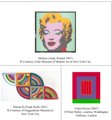
painting. Examples of artists include Richard Bowman (born in1918), Herb Aach

(1923-1985), Andy Warhol (1928-1987), Frank Stella (1936-present), and Peter Halley

(1953-present). Bowman (1973) made about 100 paintings in his “Kinetogenics” series with

fluorescent oil paints on canvas and in his “Synthesis” and ”Dynamorph” series with

fluorescent acrylic paints on canvas. Herb Aach (1970) made his “Sonic Boom” with

fluorescent paints. Andy Warhol made his “Marilyn” and “Flowers” with Day-Glo

colors. Examples of artworks containing fluorescent colors are shown in Figure 2.1.

As an aid to pigment identification, UV radiation in a darkened room can provide

information to the composition of paint layers (Carden 1991). The fluorescence effect can

be studied with a fluorescence spectrometer. Introducing fluorescent colors to the art

world posed a challenge in archiving of a painting with fluorescent colors. Hinde et al.

(2008) presented a filter-based technique to photograph the fluorescence emission of the

Day-Glo pigments. The illuminant-dependency of fluorescence spectra makes the

(41)

Marilyn (Andy Warhol 1967)

+ Courtesy of the Museum of Modern Art in New York City

Harran II (Frank Stella 1967)

+ Courtesy of Guggenheim Museum in

New York City

Violet Prison (2007)

[image:41.612.87.473.96.510.2]

+ Peter Halley, courtesy Waddington Galleries, London

Figure 2.1 Examples of artwork containing fluorescent colors.

Multipsectral imaging as a noninvasive technique has been used for archiving by

museums and cultural-heritage institutions for about a decade. This technique can provide

adequate spectral and colorimetric accuracy in making databases for museums, libraries,

and other cultural-heritage institutions. The European project VASARI (Martinez et al.

(42)

imaging project for achieving accurate color evaluation. Other research examples are the

European project named CRISATEL, the spectral imaging project in Aachen Germany

(Herzog et al.2003), and the multispectral imaging projects at the Munsell Color Science

Laboratory (MCSL) at Rochester Institute of Technology (www.art-si.org). The

European project CRISATEL was based on 10 filters within the visible spectrum (Cotte

et al.2003). The spectral imaging project in Aachen Germany is based on 16 filters

(Herzog et.al.2003). Narrow and wide-band filters have been used in the multispectral

imaging projects at the Munsell Color Science Laboratory.

In the multispectral projects performed during these years, the complex

fluorescence phenomenon has been often ignored. The ignored fluorescence would

contribute to error in digital imaging of artwork containing fluorescent colors. It is very

important to know how the fluorescence can affect the performance of a regular spectral

imaging. An interesting question is “What would be the image reproduction quality of

typical spectral imaging for color reproduction of a painting containing fluorescent colors

under different viewing illumination?”

Non-fluorescent colors can be characterized by their spectral reflected radiance

factor. This quantity is not sufficient to characterize a fluorescent color. The spectral

fluorescence, reflected and excitation spectra describe the spectral characteristic of a

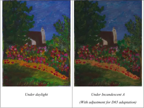
fluorescent color. The spectral reflected radiance factor is independent of illumination.

(43)

reflected and fluorescent radiance factors, is illuminant-dependent. An example of a

painting containing both fluorescent and non-fluorescent colors is shown in Figure 2.2

under daylight and incandescent light. This painting is called the “House” in the rest of

this research.

In order to achieve the correct color evaluation of fluorescent samples under a

viewing illuminant, the total radiance factor should be measured or evaluated under that

illuminant. The spectral properties of a fluorescent color can be explored using a

spectrophotometer with two monochromators, one in the irradiating beam and the other

in the viewing beam. Such a device is called a bispectrometer. The excitation, reflected

radiance, and fluorescence emission are obtained with this dual-monochromator

measurement. Output of a bispectrometer is a matrix called the Donaldson matrix after

Donaldson (1954). The diagonal of the matrix with reasonable accuracy (if the spectral

bandpass is sufficiently narrow, i.e., 1-2 nm) is the spectral reflected radiance factor and

the off-diagonal values form the fluorescent radiance factor spectra. The advantage of

measuring the excitation and emission spectra is the ability to estimate the fluorescence

emission under any desired illuminant with a good approximation. This is the most

accurate method in fluorescence colorimetry. A regular spectrophotometer with

polychromatic illumination and monochromatic detection measures the total radiance

factor under a given illuminant but it is not possible to separate the spectral reflected and

(44)

measurement is highly dependent on the similarity of the illuminants in the measuring

and viewing conditions.

Under daylight Under Incandescent A

[image:44.612.83.543.156.502.2]

(With adjustment for D65 adaptation)

Figure 2.2 Example of a painting containing both fluorescent and non-fluorescent colors under daylight and incandescent A.

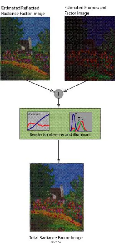
To digitally archive artwork containing both fluorescent and non-fluorescent

colors and evaluating the appearance of the painting under different illumination, the total

(45)

fluorescent colors. The total radiance factor for the non-fluorescent colors equals the

reflected radiance factor. For scenes containing fluorescent colors, capturing and

archiving the total radiance factor under different illuminants might be an accurate

approach but it is costly since it requires spectral imaging under each illuminant

separately. It would be more efficient if one could separate the reflected and fluorescent

radiance factors. In this way, one could measure the fluorescence spectrum under only

one light source and estimate the fluorescent radiance factor for other illuminants using a

proper model. Based on this method, multiple imaging under different illuminants would

not be required.

A traditional spectral imaging system consisting of a light source, a digital

camera, and an image processing model relates the detected camera signals to spectral

reflected radiance factor. Such a spectral imaging mimics a spectrophotometer; the

outputs of both systems are spectral reflected radiance factor (Mohammadi 2005). A

traditional imaging system is useful to reconstruct the total radiance factor but does not

provide the separate information about the reflectance and fluorescence spectra.

A fluorescence spectral imaging system can be developed to mimic a

bispectrometer and provide the spectral properties of the fluorescent samples. A

filter-based monochromator can be employed to generate a monochromatic beam. A set of

liquid crystal tunable filters (LCTF) in the viewing beam might produce the

monochromatic detection. Such a spectral imaging provides a good approximation of the

(46)

least 900 images (900=30 input wavelengths , 30 output wavelengths) would be

required. This would be a very difficult and impractical approach to obtain the

fluorescent properties of a painting. The goal of this dissertation was to develop an

abridged imaging bispectrometer for artwork containing both fluorescent and

non-fluorescent colors. The proposed method included two stages: reconstruction of the

spectral reflected radiance factor and reconstruction of the fluorescence spectrum. An

abridged method was developed to reconstruct a Donaldson matrix of a fluorescent color

based on a calibrated UV-fluorescence imaging system and a model was developed to

reconstruct the fluorescence spectrum. The derived matrix provided the fluorescent

radiance factor under any desired illumination. The reflected radiance factor estimation

was achieved by imaging the painting with a series of short-wavelength cutoff filters

placed in the illumination path. The goal of the filter fluorescence reduction method

(originally proposed by Eitle and Ganz, 1968) was to remove the excitation wavelengths,

which might excite fluorescence using different short-wavelength cutoff filters. It was

assumed that the detected signals by the imaging device would be transformed to spectral

reflected radiance factor. A learning-based spectral imaging system routinely used at the

Munsell Color Science Laboratory was employed to reconstruct the spectral characteristic

of the colors. A modified Sinarback 54 with six RGB channels was used as the imaging

device in all imaging steps. The main advantage of an imaging bispectrometer is the

(47)

Furthermore the spectral fluorescence emission would provide more information for

better identification and classification of materials. The other advantage of this method

was providing a general system for spectral imaging of paintings containing both

fluorescent and non-fluorescent colors. Finally, an imaging bispectrometer eliminates the

multiple imaging to obtain the total radiance factor under different light sources. A

graphical overview of the developed imaging-bispectrometer in this dissertation is shown

in Figure 2.3. The developed model was an abridged imaging bispectrometer called

abridged fluorescence spectral imaging. The goals of developing fluorescence spectral

imaging are summarized as the following:

! To characterize the spectral reflected and fluorescent radiance of the fluorescent

materials,

! To calculate the fluorescent radiance factor of a fluorescent color under any

desired illuminant,

! To estimate the total radiance factor as a summation of the reflected and

fluorescent radiance factors of a fluorescent color under any desired illuminant,

! To be employed as a general imaging system for both fluorescent and

non-fluorescent colors,

! To facilitate accurate image rendering,

! To eliminate multiple spectral imaging for different viewing illumination due to

(48)

! To provide quantitative analysis of the fluorescence emission for identification

and classification of materials,

! To evaluate the state of conservation of a work of art as a point of aging

retouching, repainting, etc.

[image:48.612.198.394.230.643.2]

(49)

Readers of this dissertation will find the background of fluorescence colorimerty

in Chapter 3. The reader will learn about the bispectrometer measurement and the ways

to calculate the quantities such as the spectral reflected, fluorescent, and total radiance

factor along with the method of calculation of the excitation spectrum in this chapter. A

new model titled as the abridged two-monochromator method developed in this

dissertation for the prediction of fluorescence emission under any desired illuminant, is

explained in detail in Chapter 4. The readers will find an exploratory experiment to

understand how to implement this method for estimating the fluorescence emission. The

interested readers in imaging will find a proper approach to image a scene containing

both fluorescent and non-fluorescent colors in Chapters 5 and 6. The comparison results

of the proposed abridged fluorescence spectral imaging, both quantitatively and visually,

with traditional spectral imaging and colorimetric imaging are presented in Chapters 6

and 7.

This dissertation might be interesting for people concerned with the fluorescence

phenomenon in fields such as art and conservation, the paper industry, and fluorescence

medical imaging. The color science students interested in understanding the concept of

fluorescence, fluorescence colorimetry, and fluorescence spectral imaging can benefit

from this document.

(50)

3

Background of Fluorescence Colorimetry

3.1

Overview

In this chapter a summarized background about fluorescence colorimetry is addressed.

Fluorescence colorimetry is a technique to evaluate the color of fluorescent materials. A

bispectrometer with two monochromators in excitation and emission paths is an accurate

instrument to evaluate the color of fluorescent samples. There are some abridged methods

to approximate the reflected and fluorescent radiance factors of these materials, which are

explained in this chapter.

The structure of this chapter is as follows:

3.2. Bispectral fluorescence colorimetry

3.3. Polychromatic and monochromatic illumination

3.4. Abridged fluorescence colorimetry

3.5. Methods for predicting the spectral total radiance factor

3.6. Requirements for fluorescence measurements

Reading this chapter gives a general idea about fluorescence and fluorescence

colorimetry. This knowledge is helpful to design a fluorescence measurement system,

(51)

3.2

Bispectral Fluorescence Colorimetry

According to ASTM E-284-03a (2004), a bispectrometer is an optical instrument

equipped with a source of irradiation, two monochromators, and a detection system, such

that a specimen can be measured at independently-controlled irradiation and viewing

wavelengths. A bispectrometer is designed to provide quantitative information of the

bispectral radiation properties of a specimen. The complete and accurate color evaluation

of fluorescent materials requires the use of a bispectrometer. Electrons of luminescent

materials absorb energy upon irradiation and go to the excited state. The excited electrons

release energy in the form of radiation in the process of returning to the ground state.

This radiation is defined as luminescence. Luminescence is a general term covering

fluorescence and phosphorescence. Fluorescence is the main focus of this dissertation.

The idea of the two-monochromator method for color evaluation of fluorescent

materials was started by Donaldson (1954) and later followed by Costa and Grum (1969).

The spectrophotometers used in this method had two monochromators, one in the

irradiating beam and the other in the viewing beam. The geometry of such a

spectrophotometer was usually 45/0. The advantage of this method is the capability of

measuring the various qualities such as reflectance, fluorescence, and excitation spectra.

The excitation spectrum of a sample could be obtained by setting the monochromator in

the viewing beam to wavelength, ', in the emission region and scanning through the

excitation region using the other monochromator. The fluorescence spectrum could be

(52)

excitation region and scanning through the emission region by the other monochroamtor.

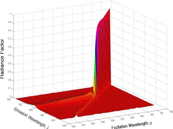
The spectral radiance emitted by a fluorescent sample at any given wavelength depends

on both incident or excitation wavelength (µ) and emission wavelength ('). The ratio of

spectral radiance at wavelength ' when irradiated at wavelength µ to the total radiance of

a perfectly reflecting diffuser similarly irradiated and viewed is defined as the bipsectral

radiance factor. A bispectral radiance factor of Golden! fluorescent orange measured by

a Labsphere BFC-450 bispectrometer for an interval of 10 nm is shown in Figure 3.1.

The same data in the form of a matrix, DT, sampled at 50 nm intervals are listed in Table

3.1. As an example, a measurement corresponding to an excitation at 400 nm and

emission at 600 nm DT(600,400), a value of 0.03, is presented in the fifth row and the

third column. A radiance factor of 0.03 was obtained for a measurement at 600nm for an

incident light at 400nm. The summation of this matrix over the excitation wavelengths

results in the total radiance factor. For example, summation of the elements of the fifth

row corresponding to the emission wavelength of 600 nm results in the total radiance

factor of 0.51. Hereafter the matrix format of a bispectral radiance factor, DT, presented

in Table 3.1, is called the Donaldson matrix after Donaldson (1954). The subscript “T”

(53)

[image:53.612.111.411.360.585.2]

Table 3.1 Total radiance factor values, Donaldson radiance factor matrix, for Golden! fluorescent orange measured by a Labsphere BFC-450. (Values less than 0.01 have been set to zero.)

Excitation wavelength

300 350 400 450 500 550 600 650 700 750

Total Radiance Factor

400 0 0 0.04 0 0 0 0 0 0 0 0.04

450 0 0 0 0.03 0 0 0 0 0 0 0.03

500 0 0 0 0 0.04 0 0 0 0 0 0.04

550 0 0 0 0 0 0.03 0 0 0 0 0.03

600 0.02 0.02 0.03 0.03 0.04 0.04 0.34 0 0 0 0.51

650 0.01 0.01 0.02 0.02 0.03 0.03 0.03 0.88 0 0 1.03

700 0 0 0 0 0 0 0 0 0.88 0 0.88

E

m

is

si

on

Wa

ve

le

n

gt

h

750 0 0 0 0 0 0 0 0 0 0.91 0.91

Figure 3.1 The Donaldson radiance factor matrix for Golden! _{fluorescent orange}

(54)

A Donaldson matrix can be considered as the summation of two components,

reflected and luminescence radiance factor matrices denoted by DR andDL in Eq 3.1,

respectively.

!

DT

(

",µ

)

#DR

(

",µ

)

+DL

(

",µ

)

( 3.1)

By a good approximation (if the spectral bandpass is sufficiently narrow, i.e., 1-2

nm), values of the diagonal elements ('=µ) represent the reflected radiance factors. The

matrix of the reflected radiance factors, DR, for Golden! fluorescent orange is shown in

Table 3.2. Setting the diagonal values ('*µ) of the Donaldson matrix to zero values

results in the Donaldson luminescence radiance factor matrix, DL, (e.g. Table 3.3).

Table 3.2 A reflected radiance factor matrix corresponding to Donaldson matrix listed in

Table 3.1 for Golden! fluorescent orange measured by a Labsphere BFC-450.

Excitation wavelength, µ

300 350 400 450 500 550 600 650 700 750

Reflected Radiance Factor

400 0 0 0.04 0 0 0 0 0 0 0 0.04

450 0 0 0 0.03 0 0 0 0 0 0 0.03

500 0 0 0 0 0.04 0 0 0 0 0 0.04

550 0 0 0 0 0 0.03 0 0 0 0 0.03

600 0 0 0 0 0 0 0.34 0 0 0 0.34

650 0 0 0 0 0 0 0 0.88 0 0 0.88

700 0 0 0 0 0 0 0 0 0.88 0 0.88

E m is si on w av el en gt h

(55)

Table 3.3 A fluorescent radiance factor matrix corresponding to Donaldson matrix listed

in Table 3.1 for Golden! fluorescent orange measured by a Labsphere BFC-450 (Values

less than 0.01 have been set to zero.)

Excitation wavelength

300 350 400 450 500 550 600 650 700 750

Fluorescent Radiance Factor

400 0 0 0.00 0 0 0 0 0 0 0 0.00

450 0 0 0 0.00 0 0 0 0 0 0 0.00

500 0 0 0 0 0.00 0 0 0 0 0 0.00

550 0 0 0 0 0 0.00 0 0 0 0 0.00

600 0.02 0.02 0.03 0.03 0.04 0.04 0.00 0 0 0 0.17

650 0.01 0.01 0.02 0.02 0.03 0.03 0.03 0.00 0 0 0.15

700 0 0 0 0 0 0 0 0 0.00 0 0.00

E m is si on Wa ve le n gt h

750 0 0 0 0 0 0 0 0 0 0.00 0.00

Excitation

Factor 0.03 0.03 0.04 0.05 0.06 0.07 0.03 0.00 0.00 0.00

The fluorescence emission and excitation spectra are the spectral fluorescence

characteristic of a fluorescent color. This information is encapsulated in the Donaldson

luminescence radiance factor matrix DL. The summation of DL over the excitation

wavelengths gives results in the fluorescent radiance factor, F(') (The last column in

Table 3.3). For example, summation of the elements of the fifth row corresponding to the

emission wavelength of 600 nm results in a fluorescent radiance factor of 0.17. The

summation over the emission wavelength gives the excitation factors, X(µ), which are

shown in the last row of the Table 3.3 (the last row in Table 3.3.) As an example, the

excitation factor at 400 nm was calculated by summation over the third column, which

(56)

Figure

+7

References

Download now ( PDF - 332 Page - 12.02 MB )

Outline

Methods for Predicting Spectral Total Radiance Factor Introduction Results and Discussions Filter-Based Abridged Fluorescence Reduction Methods Virtual Camera Results and Discussion Image Acquisition System Geometry of Imaging

Developing an imaging bi-spectrometer for fluorescent materials

Rochester Institute of Technology

RIT Scholar Works

Developing an Imaging Bi-Spectrometer for Fluorescent Materials

CHESTER F. CARLSON CENTER FOR IMAGING SCIENCE ROCHESTER INSTITUTE OF TECHNOLOGY

DISSERTATION RELEASE PERMISSION ROCHESTER INSTITUTE OF TECHNOLOGY

Developing an Imaging Bi-Spectrometer for Fluorescent Materials

Abstract

ACKNOWLEDGMENTS

DEDICATION

Table of Contents

4 Prediction of Fluorescence Emission, A New Model... 52

6 Image-Based Abridged Fluorescence Spectral Imaging ... 140

7 Visual Evaluation of the Imaging Models... 239

List Of Figures

List Of Tables

Terminology

Introduction

Background of Fluorescence Colorimetry

Bispectral Fluorescence Colorimetry

Excitation wavelength

Reflected Radiance Factor